Article

A Method for Identifying Gross Errors in Dam Monitoring Data

1
The National Key Laboratory of Water Disaster Prevention, Hohai University, Nanjing 210098, China
2
College of Water Conservancy and Hydropower Engineering, Hohai University, Nanjing 210098, China
3
National Engineering Research Center of Water Resources Efficient Utilization and Engineering Safety, Hohai University, Nanjing 210098, China
*
Author to whom correspondence should be addressed.
Water 2024, 16(7), 978; https://doi.org/10.3390/w16070978
Submission received: 28 February 2024 / Revised: 23 March 2024 / Accepted: 25 March 2024 / Published: 28 March 2024

Abstract

:
Real and effective monitoring data are crucial in assessing the structural safety of dams. Gross errors, resulting from manual mismeasurement, instrument failure, or other factors, can significantly impact the evaluation process. It is imperative to eliminate such anomalous data. However, existing methods for detecting gross errors in concrete dam deformation often focus on analyzing a single monitoring effect quantity. This can lead to sudden jumps in values of effect quantity caused by changes in environmental variables being mistakenly identified as gross error. Therefore, a method based on Fuzzy C-Means clustering algorithm (FCM) partitioning and density clustering algorithm (Ordering Points To Identify the Clustering Structure, OPTICS) combined with Local Outlier Factor (LOF) algorithm for gross error identification is proposed. Firstly, the FCM algorithm is used to achieve the division of measurement point areas. Then, the OPTICS and LOF algorithms are jointly utilized to determine the gross errors. Finally, the real gross errors are identified by comparing the time of occurrence of the gross errors at measurement points in the same area. Through the case study, the results indicate that the method can effectively identify spurious, gross errors in the monitoring effect quantity caused by environmental mutations. The accuracy of gross error detection is significantly improved, and the rate of misjudgment of gross errors is reduced.

1. Introduction

To avoid sudden dam diseases in the service process, which may lead to serious engineering accidents and cause significant loss of life and property, it is essential to continuously monitor the operational status of the dam body in real-time. Regular analysis of monitoring data, including deformation, seepage, and uplift pressure, allows for a comprehensive understanding of the dam’s health status and ensures its long-term stable operation [1,2,3]. Accurate monitoring data are an important prerequisite and fundamental guarantee for effective dam safety monitoring. Therefore, the preprocessing of dam monitoring data is necessary.
The original data from concrete dam safety monitoring often includes gross errors resulting from reading errors, instrument failures, and other factors. These errors represent unreasonably inaccurate data points that can significantly distort dam monitoring data. If not effectively addressed, they can compromise the accuracy of safety evaluations, early warnings, and forecasts for the dam. Consequently, eliminating gross errors is an important part of preliminary processing [4,5,6]. To identify gross errors, many scholars have carried out related research. Traditional gross error identification methods are generally based on statistical theories, such as 3σ criterion, Grubbs criterion, Romanowski criterion, and Dixon criterion, which have been widely employed for gross error identification in dam monitoring data [7,8,9,10]. However, when the structure of dam monitoring data is complex, problems of missing judgment and misjudgment are easy to occur. As a result, many scholars have endeavored to enhance traditional methods, aiming to improve the detection rate. For example, Zhao et al. [11] proposed an improved 3σ criterion based on the Minimum Covariance Determinant. Li et al. [12] introduced an enhanced Pauta criterion based on M estimation. With the development of big data analysis technology, machine learning has also been gradually applied to gross error recognition [13]. Examples include Neural Networks [14,15], Support Vector Machines [16,17], Decision Trees [18,19], and others. Song et al. [20] proposed a gross error detection method of singular spectrum analysis (SSA) combined with nonlinear autoregression (NAR). Qi et al. [21,22] used full convolutional networks to learn from artificially labeled datasets and realize the recognition of gross error data. Hu et al. [23] proposed a method for identifying anomalies by combining dynamic time warping with a local outlier factor. Song et al. [24] developed an analysis method for detecting outliers in dam deformation data based on multivariable panel data and K-means clustering theory. Shao et al. [25] converted monitoring data into images and processed outliers in combination with the cuckoo-search algorithm. Bao et al. [26] visualized time series data and fed them into a deep neural network to detect anomalous data [27,28,29]. Zhang et al. [30] integrated multiple learners and proposed an anomaly diagnosis method using an anomaly index matrix updated with real-time data. Gu et al. [31] used an improved IGG method and an extreme learning machine to identify gross errors in deformation monitoring data. Li et al. [32] proposed an outlier identification method based on a BP neural network. Liu et al. [33] utilized the wavelet transform to identify outliers in time series data. While these methods have shown success in identifying gross errors, many of them are computationally complex. Moreover, several primarily rely on time series change rules and fail to fully consider the influence of environmental changes on dam behavior. Typically, significant fluctuations in environmental factors such as water levels and temperature can lead to corresponding variations in key parameters like deformation. These variations represent the actual behavior of the dam, providing valuable data reflecting its true state. However, they are prone to being misinterpreted as gross errors.
To address the aforementioned issues, the local density difference between normal data and data containing gross errors is considered in this paper, and a method for identifying gross errors in dam safety monitoring data is presented. This method combines FCM clustering, OPTICS, and LOF algorithms. Firstly, the FCM algorithm is applied to partition the dam displacement measurement points, followed by the use of an enhanced OPTICS algorithm for preliminary gross error identification. Subsequently, the LOF value of each data point in the preliminary gross error dataset is calculated. If the LOF value exceeds a predefined threshold, the data is flagged as a gross error. Finally, potential misjudgments resulting from changes in environmental quantities are mitigated by comparing the data with other measurement points within the same cluster, ultimately determining the final classification of gross errors. The combination of OPTICS and LOF algorithms significantly enhances the accuracy and sensitivity of gross error detection while also reducing the rate of misjudgments to some extent. Because the proposed method only calculates LOF values for a subset of the data, it can effectively reduce computational complexity.

2. Fundamentals of a Gross Error Identification Algorithm for Dam Monitoring Data

2.1. FCM Algorithm

The Fuzzy C-means (FCM) clustering algorithm introduces fuzzy set theory into cluster analysis. Instead of categorizing sample data into a specific partition with 100% certainty, it calculates the membership degree of each data sample corresponding to each class by optimizing the objective function. This approach achieves optimal data clustering, effectively enhancing the algorithm’s resistance to noise and its overall fuzziness [34,35]. To obtain accurate clustering results, it is necessary to comprehensively analyze the change trend of the measured value series. Therefore, the comprehensive distance, a weighted combination of absolute distance, incremental distance, and growth rate distance, is adopted as the similarity index [36]. The indicators are explained as follows.
(1) The absolute distance between the measuring point i and the measuring point j , denoted d i j ( A D ) .
d i j ( A D ) = t = 1 T δ i t δ j t 2 1 2
where δ i t is the deformation value of the measuring point i at time t; δ j t is the deformation value of the measuring point j at time t.
(2) The incremental distance between the measuring point i and the measuring point j is denoted as d i j ( K D ) .
d i j ( K D ) = t = 1 T Δ δ i t Δ δ j t 2 1 2
where Δ δ i t = δ i t δ i t 1 ; Δ δ j t = δ j t δ j t 1 .
(3) The growth rate distance between the measuring point i and the measuring point j is denoted as d i j ( G R D ) .
d i j ( G R D ) = t = 1 T Δ δ i t δ i t 1 Δ δ j t δ j t 1 2 1 2
(4) The comprehensive distance between the measuring point i and the measuring point j is denoted d i j ( C E D ) .
d i j ( C E D ) = ω 1 d i j ( A D ) + ω 2 d i j ( K D ) + ω 3 d i j ( G R D )
where ω 1 , ω 2 and ω 3 represent the weight coefficients of the three distances, which meet the requirement that ω 1 + ω 2 + ω 3 = 1 . This paper adopts the entropy weight method [37] for their calculation.
Assuming that the concrete dam has n deformation measurement points, x 1 , x 2 , , x n , and the number of clusters is c, then the objective function of FCM is as follows:
min J m ( U , c ) = j = 1 c i = 1 n u i j m d x i v j ( C E D )
where U is the membership matrix, U = [ u i j ] c × n ; u i j is the membership degree of the measuring point x i and cluster center v j ; m is the fuzzy index and the best value interval is [1.5, 2.5]; d x i v j ( C E D ) is the comprehensive distance between the measuring point x i and cluster center v j .
The specific steps of the FCM algorithm are as follows:
Step 1: Set the fuzzy index m and cluster number c , initialize the membership matrix U 0 , set the convergence accuracy ε > 0 , and calculate the comprehensive distance between the measurement points.
Step 2: Calculate cluster centers v j :
v j = i = 1 n u i j m x i / i = 1 n u i j m
Step 3: Update the membership matrix U :
u i j = k = 1 c d x i v j d x i v k 2 / ( m 1 ) 1
Step 4: Repeat steps 2 and 3 until the difference in membership matrices between consecutive iterations is less than the set threshold ε .
In this paper, the Silhouette Coefficient method is employed to determine the optimal number of clusters ( c ). Various values of c are utilized for clustering, and the corresponding silhouette coefficients are calculated. The silhouette coefficient (S) ranges between [–1, 1], and the closer it is to 1, the better the clustering effect. The silhouette coefficient S i for a single measurement point x i is defined as follows:
S i = p ( x i ) q ( x i ) max { q ( x i ) , p ( x i ) }
where p ( x i ) is the average distance between measuring point x i and other measuring points within the same cluster; q ( x i ) is the minimum value of the average distance between measuring point x i and the samples of other clusters.

2.2. OPTICS Algorithm and Its Improvement

2.2.1. OPTICS Algorithm

Ordering Points To Identify the Clustering Structure (OPTICS) is a density-based clustering algorithm, which is an improvement of DBSCAN [38]. Compared with DBSCAN, although the neighborhood radius ( ε ) and the minimum number of neighborhood points ( M i n P t s ) must be set, OPTICS achieves clustering results that are less dependent on the selection of ε and M i n P t s . It obtains a series of parameter-set density-based clusterings by introducing the core-distance and reachability-distance [39,40]. The OPTICS algorithm is capable of effectively handling datasets with non-uniform density, unlike other algorithms that require all clusters to possess similar densities. The fundamental concept behind OPTICS is to initiate a random selection of data and expand towards the densest area. Each data point has a reachability-distance to represent its density relationship with other data points. Based on the reachability-distance of each data point, an accessible distance map is generated, reflecting the density of the data. The relevant definition of the algorithm is as follows:
Definition 1. 
Neighborhood radius ( ε ): Given a data set  D , for any point  p  in  D , the neighborhood radius is defined as a circular region with the point  p  as the center and  ε  as the radius.
Definition 2. 
Minimum number of neighborhood points ( M i n P t s ): The minimum number of points within the neighborhood radius required for a point to be considered a core point.
Definition 3. 
Core point: The core point has at least  M i n P t s  data points in the neighborhood radius.
Definition 4. 
Core-Distance: The minimum neighborhood radius of a point that makes it a core point, that is, the distance from it to the  M i n P t s  closest point in its neighborhood. If a point is not a core point, its core-distance is undefined.
Definition 5. 
Reachability-Distance: The reachability-distance from one point  q  to another core point  p  is  M a x ( c o r e D i s t ( p ) , d ( p , q ) ) , which is the greater value between the distance from  q  to  p  and the core-distance of  p . If  p  is not a core point, then the reachability-distance from  q  to  p  is undefined.  d ( p , q )  represents the distance between  p  and  q .
Definition 6. 
Direct Density Reachability: If the reachability-distance from a point  q  to another core point  p  is less than or equal to  ε , and  q  is in the neighborhood radius of  p , then it is said to have direct density reachability from  p  to  q .
The core-distance and reachability-distance are shown in Figure 1. Given the neighborhood radius ε = 6 and the minimum number of neighborhood points M i n P t s = 5 , then the core-distance of p is 3, the reachability-distance from q to p is max ( c o r e D i s t ( p ) , d ( p , q ) ) = 7 , and the reachability-distance from r to p is max ( c o r e D i s t ( p ) , d ( p , r ) ) = 3 .
In the clustering process, OPTICS uses two queues: an ordered seed queue and a result queue. The orderly seed queue is used to temporarily store the points to be processed and is arranged in ascending order according to the reachability-distance. The data points with the smallest reachability-distance are preferentially selected for processing, and the data points are expanded to the densest area of data. In this way, data objects with high density can be quickly found. The result queue is used to store the output data points and is arranged in descending order of reachability-distance to form a decision graph. On the decision graph, the regions of steep rises and steep falls can be identified, representing the anomalous points and the points inside the cluster, respectively.

2.2.2. Improved OPTICS Algorithm

Although the clustering results are minimally affected by the setting of the parameters, and the number of clusters does not need to be specified in advance, the time complexity is quite high. When data is selected from the ordered seed queue for expansion, the core-distance and reachability-distance are calculated for any point in its neighborhood. If a data point is already in the seed sequence and the reachability-distance is greater than the calculated result, the original data is replaced and reordered. If it does not belong to the seed sequence, it is added to the corresponding position of the seed sequence according to its reachability-distance. The fastest sorting algorithm is used to perform the above sorting, and the time complexity of each data added or updated in the seed sequence is O ( n log n ) .
Because of the high time complexity of the OPTICS algorithm, a non-sorted seed sequence is adopted to improve the efficiency of the algorithm [41]. A temporary variable repository is created to store data points with the minimum reachability-distance in the seed sequence, which is no longer sorted by the reachability-distance. When the seed sequence adds or updates a point, simply compare the size of the reachability-distance with the temporary variable and replace the temporary variable if it is smaller. When a point needs to be extracted from the seed sequence, it is only necessary to extract the point from the temporary variable repository. Subsequently, identify the new minimum reachability-distance point from the seed queue and store it in the temporary variable repository. Compared with sorting, this method of traversing the seed queue to find the minimum point greatly improves efficiency, and the time complexity of traversing a seed sequence is O ( n ) . The specific implementation steps of the algorithm are as follows:
Step 1: Create a seed queue, a result queue, and a temporary variable repository. The seed queue is designed to store a large number of samples to be processed, and the result queue is intended for storing samples after processing. The temporary variable repository is utilized to store the next sample to be processed.
Step 2: An unprocessed core point is randomly selected and placed into the result queue. At the same time, the reachability-distance of sample points in its neighborhood is calculated. Add these sample points to the seed queue, selecting the sample with the minimum reachability distance and placing it in the temporary variable repository.
Step 3: If the seed queue is empty, return to step 2 (reselect the data). Otherwise, extract the sample p from the temporary variable repository. If p is not a core point, the fourth step is performed. If p is a core point, expand any unexpanded data q in its neighborhood ε and calculate its reachability-distance. If q is already in the seed queue and the new reachability-distance is less than the original value, update the reachability-distance. If q is not in the seed queue, it is placed in the seed queue.
Step 4: The p is written into the result queue, and the sample points with the smallest reachability-distance are re-found in the seed queue and put into the temporary variable repository. Repeat step 3 until all points in the data set are processed. Then, the algorithm ends, and the ordered sample points in the result queue are output.

2.3. LOF Algorithm

The LOF algorithm is a method for determining whether a sample is abnormal according to the ratio of the local density of a sample to that of its neighbors [23]. The outlier degree of data is determined by calculating the outlier factor of each data sample. The greater the outlier factor value, the higher the likelihood that the sample is abnormal data. Moreover, the algorithm is capable of computing the LOF values for specified data points without the need to traverse all data points, thus significantly reducing computational complexity. The related concepts of the algorithm are as follows:
Definition 7. 
The distance  d b ( a )  between object  a  and object  b : the distance between point  a  and its  b -th nearest neighbor.
Definition 8. 
The  b -th distance neighborhood of an object  a  (denoted as  N b ( a ) ): the set of data points whose distance from  a  is less than or equal to  d b ( a ) .
Definition 9. 
Reachability-Distance: The reachability-distance from object  a  to object  ο  is the greater of the  d b ( o )  and the direct distance between object  ο  and  a , i.e.,:
r e a c h distance b ( a , ο ) = max d b ( ο ) , d ( a , ο )
Definition 10. 
Locally Reachable Density: The locally reachable density of an object  a  is defined as the reciprocal of the average reachability-distance from each point in the  N b ( a )  to  a , i.e.,:
l r d b ( a ) = 1 / ο N b ( a ) r e a c h d i s t b ( a , ο ) N b ( a )
Definition 11. 
Local Outlier Factor (LOF): The local outlier factor of an object  a  is defined as the average of the ratio of the locally reachable density of  N b ( a )  to the locally reachable density of  a , i.e.,
L O F b ( a ) = ο N b ( a ) l r d b ( ο ) l r d b ( a ) N b ( a )
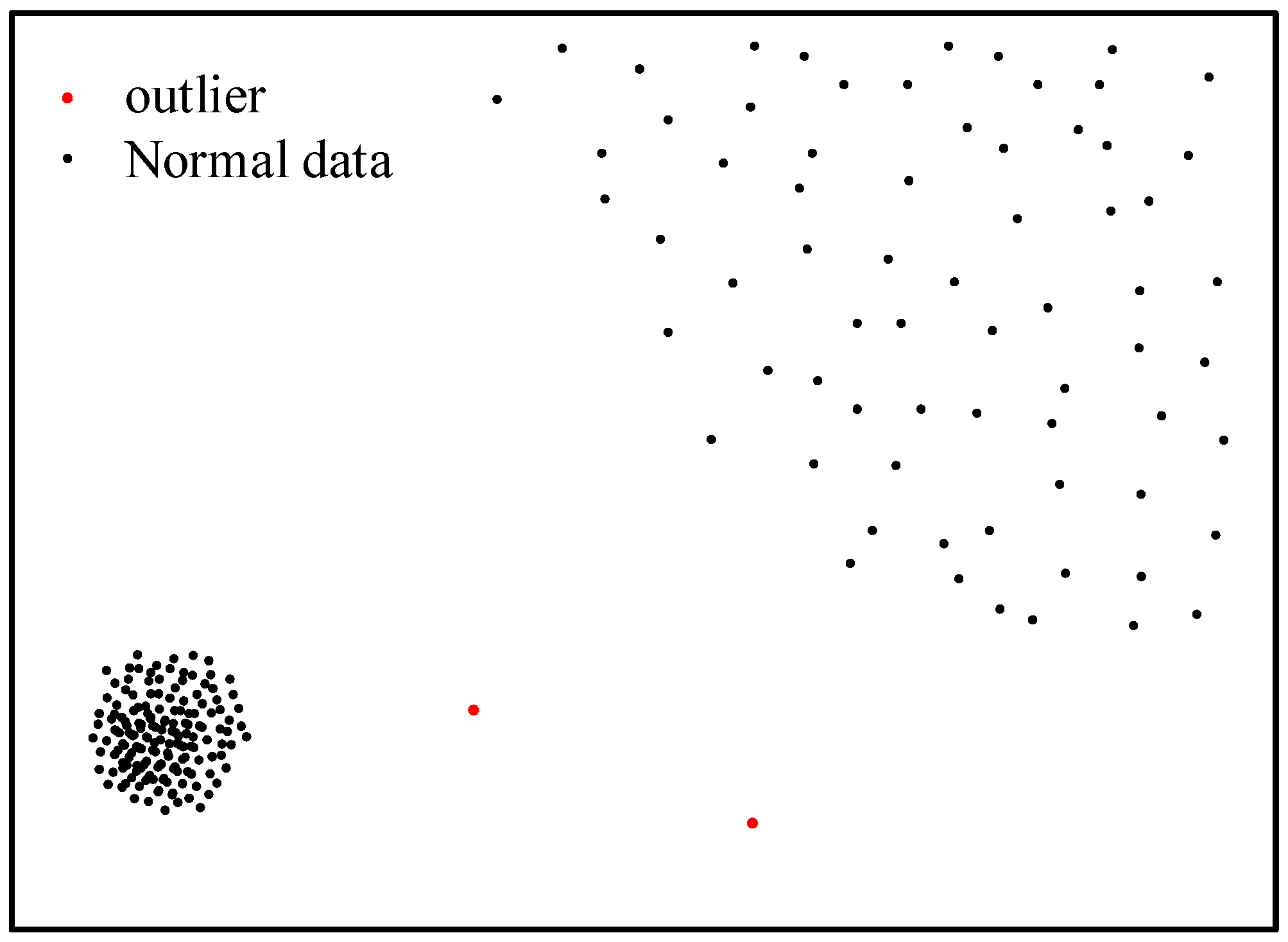
Figure 2 shows a schematic diagram of the LOF algorithm identifying a few outliers in the sample.

3. Gross Error Identification Method for Dam Safety Monitoring Based on FCM-OPTICS-LOF Algorithm

The dam body undergoes displacement due to water pressure, temperature, and aging effects. While the displacement magnitude varies at different measuring points, there is a certain commonality in the load received. As a result, several measuring points may exhibit similar deformation patterns. Therefore, the FCM clustering algorithm is employed to partition the dam measuring points based on deformation, ensuring that measuring points within each region share similar deformation process lines. Subsequently, the OPTICS clustering algorithm, combined with the LOF algorithm, is utilized to identify gross errors in the monitoring data.
In the reachability-distance diagram of OPTICS, the abscissa represents the order of the output data points, and the ordinate represents the reachability-distance. A point with a larger reachability-distance indicates lower data density and a higher likelihood of gross error. Typically, gross errors constitute only a small portion of the overall data. Therefore, data at the top ρ % of the reachability-distance (where ρ is the selected percentage) are treated as preliminary gross errors. Following this, the LOF value of each data point in the preliminary gross errors is calculated, and data with an LOF value greater than the threshold are identified as gross errors. On the basis of identifying gross errors with the OPTICS algorithm, the LOF algorithm is further used to detect local abnormalities in data. This multi-level gross error identification method can be applied to various types of data sets and reduce the missed detection rate.
However, data points with low densities may also be true values characterizing the normal operating conditions of the dam due to changes in environmental quantities (e.g., water level). To address this, it is necessary to identify the gross errors of other measurement points located in the same zone but on different vertical lines, and the appearance time of the gross errors should be compared. If a measurement point is detected with gross errors at a certain moment while other measurement points in the same area at this moment are valid, it is judged as a gross error. If two measurement points exhibit gross errors simultaneously, then it is considered that the anomaly is the real value caused by the change in environmental quantity. Thus reducing the misjudgment rate. The specific implementation process of the method is shown in Figure 3.

4. Case Study

4.1. Project Overview

A certain concrete hyperbolic arch dam is located in Sichuan Province, China, with a maximum dam height of 305 m. The dam crest elevation is 1885 m, and the lowest elevation of the foundation is 1580 m. A total of 29 vertical displacement monitoring points are arranged in the dam sections #5, #9, #11, #13, #16, and #19 to monitor the deformation of the dam body. To validate the effectiveness of the proposed gross error identification method in this paper, displacement monitoring data from the dam are selected for analysis for the period from 1 September 2015, to 31 December 2018. Figure 4 shows a photograph of the hyperbolic arch dam.

4.2. Clustering Partition

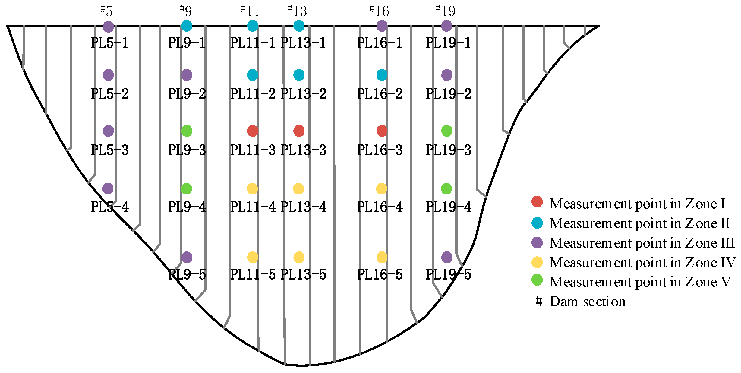
The FCM clustering algorithm is employed to assess the similarity in the deformation of the 29 measurement points. The range of clusters ( c ) is set from 3 to 10, and the silhouette coefficient is computed for each cluster. As illustrated in Figure 5, when the number of clusters ( c ) is set to 5, the silhouette coefficient reaches its maximum value of 0.64. At this point, the samples within the cluster demonstrate high aggregation, and there is significant separation between samples belonging to different clusters. Consequently, we select c = 5 as the optimal number of clusters. The dam partitioning results are displayed in Figure 6.

4.3. Gross Errors Identification

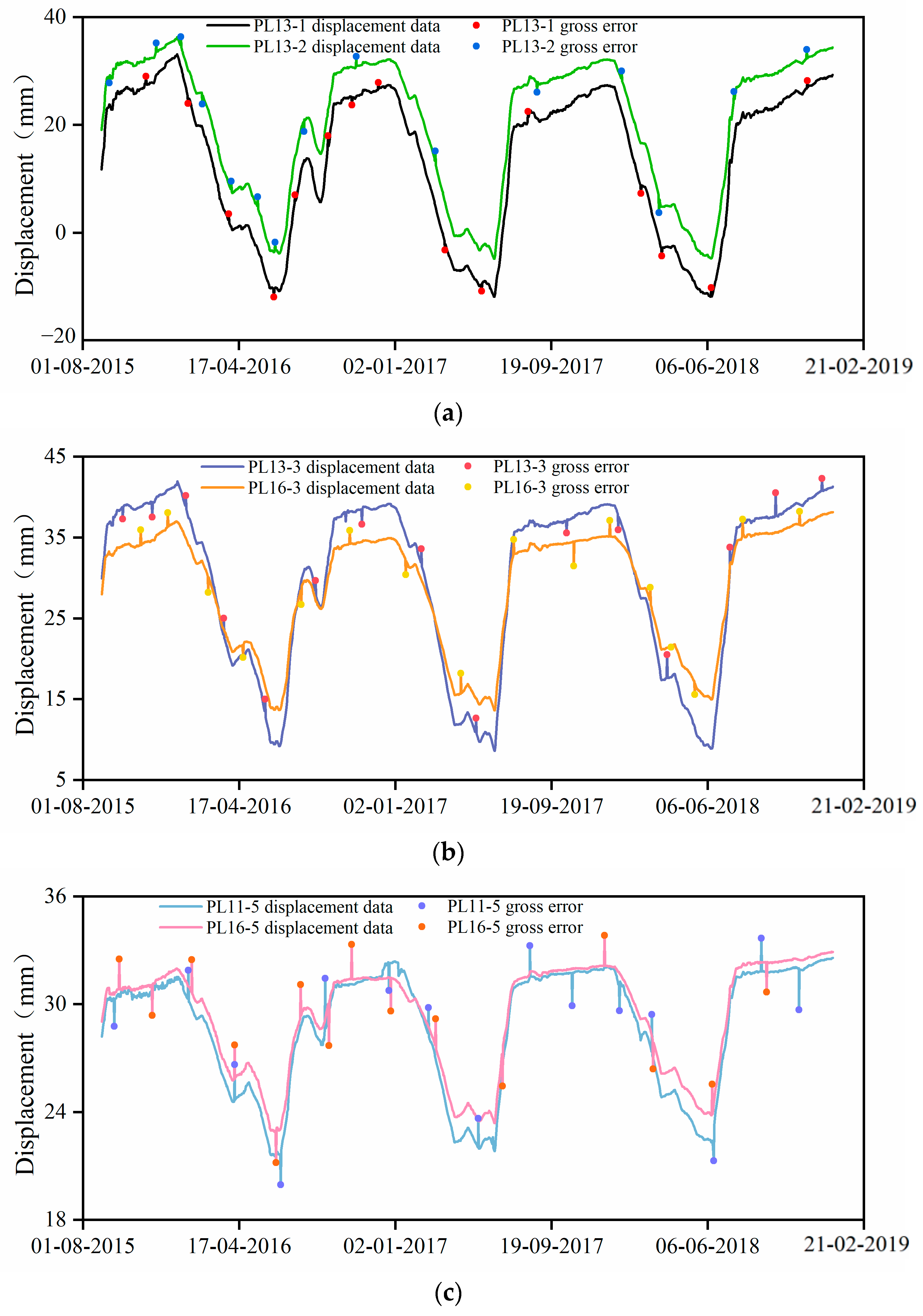
This section selects displacement monitoring data from typical monitoring points PL13-1 and PL13-2 in Zone Ⅱ, PL13-3 and PL16-3 in Zone Ⅰ, as well as PL11-5 and PL16-5 in Zone Ⅳ of the dam for the purpose of outlier (gross error) identification verification. In each displacement dataset, 15 artificial gross error data points are introduced. The specific locations and values of the introduced outliers for PL13-1 and PL13-2 are presented in Table 1 (the remaining four monitoring points are shown in Table A1 and Table A2 in Appendix A). The displacement time series for each zone after introducing outliers are illustrated in Figure 7.
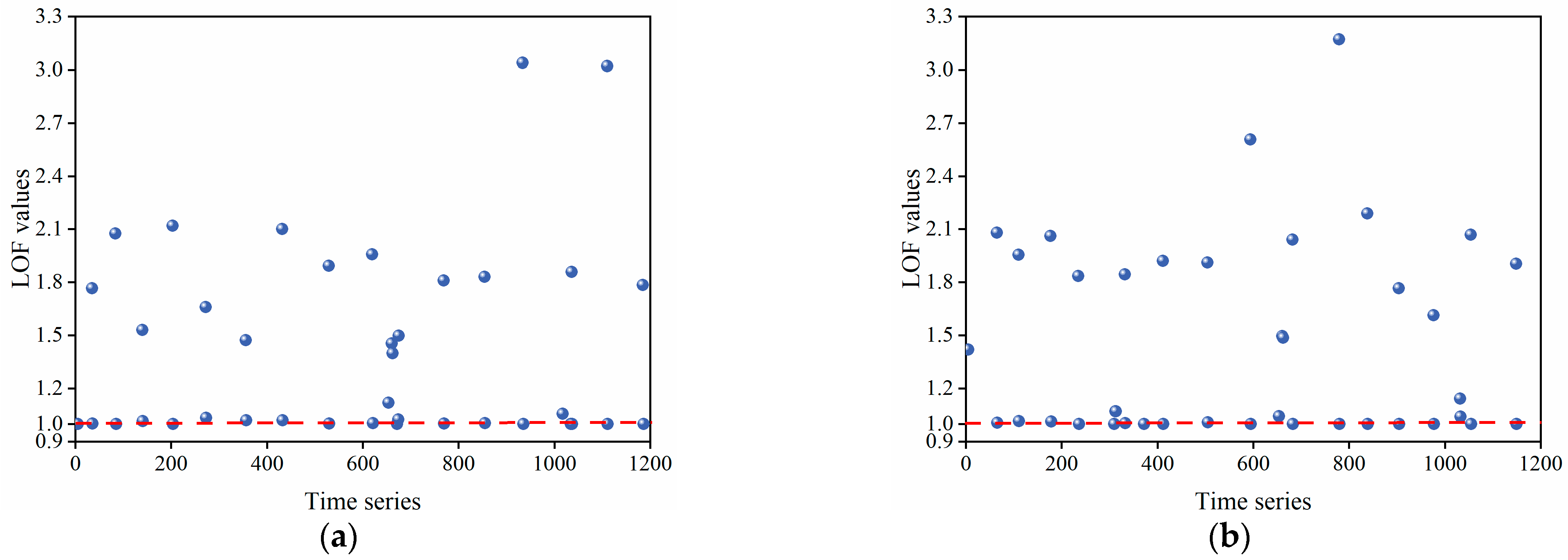
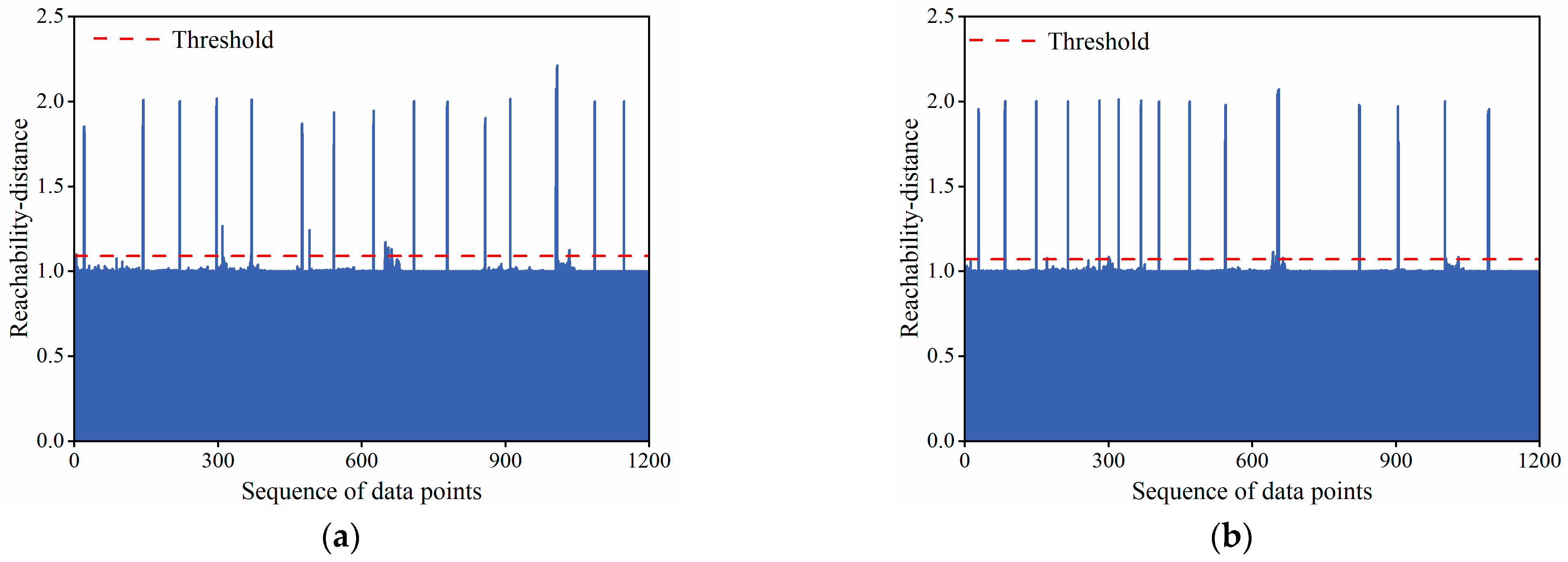
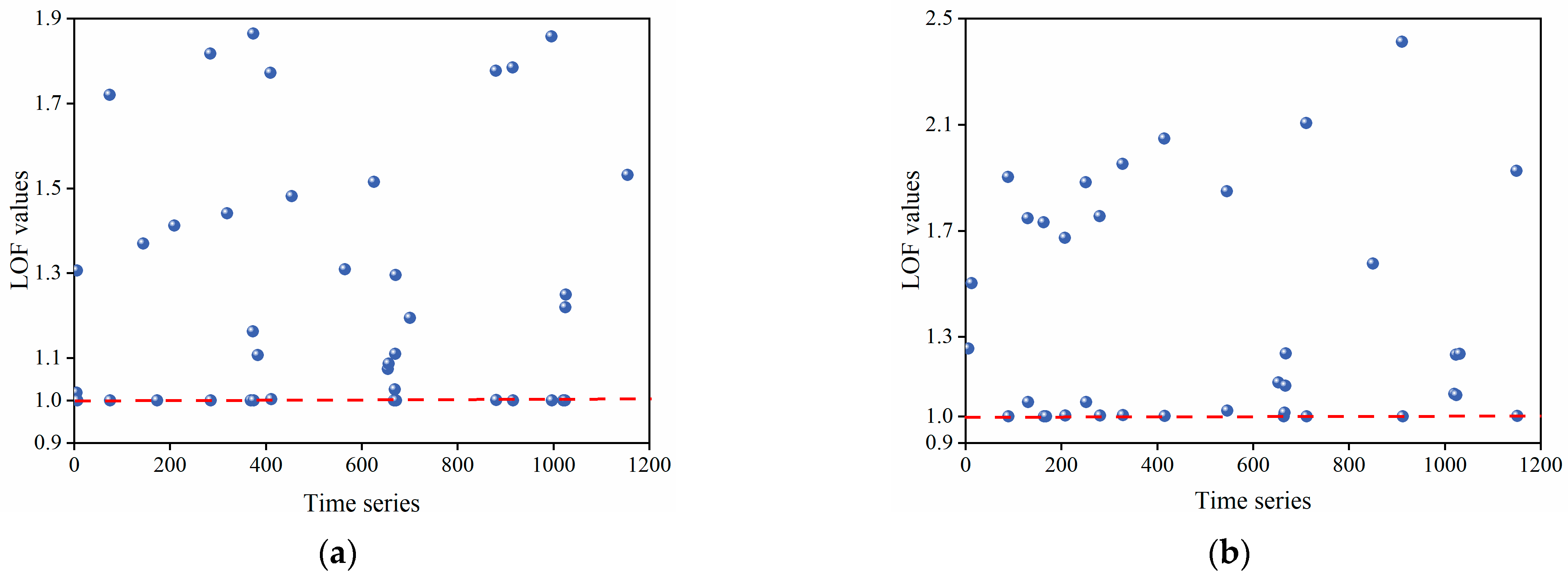
Utilizing the OPTICS algorithm, clustering analysis is performed on the displacement data from monitoring points PL13-1 and PL13-2. Given that gross errors constitute only a small portion of the data, the preliminary gross errors are selected based on the top 4% [41] of reachability-distance. The reachable distance plots for the two monitoring points are shown in Figure 8. The LOF values for each data point in the preliminary gross errors are then computed. Notably, some data points exhibited LOF values significantly greater than 1, designating them as gross errors. The scatter plot of LOF values for the monitoring points is illustrated in Figure 9.
Considering the quantity of data and the distribution of LOF values, the first 20 data points are identified as outliers. For monitoring point PL13-1, aside from the 15 intentionally introduced anomalies, data points on 7 September 2015, 11 September 2016, 12 July 2017, 11 July 2018, and 12 July 2018 are also flagged as outliers. Similarly, intentional anomalies introduced to PL13-2 are successfully identified, and additional outliers are detected on 7 September 2015, 27 June 2017, 11 July 2017, 12 July 2017, and 11 July 2018. To ascertain the final genuine outliers, a comparison of the occurrence time of abnormal data between PL13-1 and PL13-2 is conducted. Considering the slight lag in the response of monitoring points at different positions on the dam when subjected to environmental factors, the displacement data on 7 September 2015, 12 July 2017, 11 July 2018, and 12 July 2018 for PL13-1, as well as the data on 7 September 2015, 11 July 2017, 12 July 2017, and 11 July 2018 for PL13-2, are determined not to be outliers. Instead, they represent measured data reflecting actual dam displacement changes due to environmental variations and require no further processing.
Similarly, gross error identification is conducted for monitoring points PL13-3 and PL16-3 in Zone Ⅰ, as well as PL11-5 and PL16-5 in Zone IV (see Figure A1, Figure A2, Figure A3 and Figure A4 in Appendix A). For all monitoring points, the 15 intentionally introduced outlier data points are accurately identified. Furthermore, at PL13-3, data points on 27 June 2017, 28 June 2017, and 11 July 2017 are identified as gross errors. Similarly, at PL16-3, data points on 6 September 2015, 28 June 2017, and 11 July 2017 are flagged as gross errors. However, through comparative analysis, it is determined that the three data points for PL13-3, as well as the data points on 28 June 2017, and 11 July 2017, for PL16-3, are not gross errors. For Zone IV, outlier identification is performed on monitoring points PL11-5 and PL16-5. After the comparison of gross error positions, three points marked as gross error in each of the two measuring points are subsequently identified as normal points.
The above analysis reveals that the FCM-OPTICS-LOF gross error identification method can accurately detect intentionally introduced anomalous data. By employing a comparative approach with similar monitoring points, the anomalous data can be effectively categorized into gross errors and points reflecting the dam’s operational state, thereby minimizing misclassifications. This validates the effectiveness and accuracy of the proposed gross error identification method in this study.

4.4. Comparison Analysis with Other Identification Methods

To prove the superiority of the FCM-OPTICS-LOF gross error identification method proposed in this paper, we compare and analyze the gross error identification effects of FCM-LOF, FCM-DBSCAN, and the method proposed in this paper. The correct rate is used as the evaluation index:
c o r r e c t   r a t e = T N
where N represents the number of gross errors identified by the algorithm; T is the number of gross errors intentionally added.
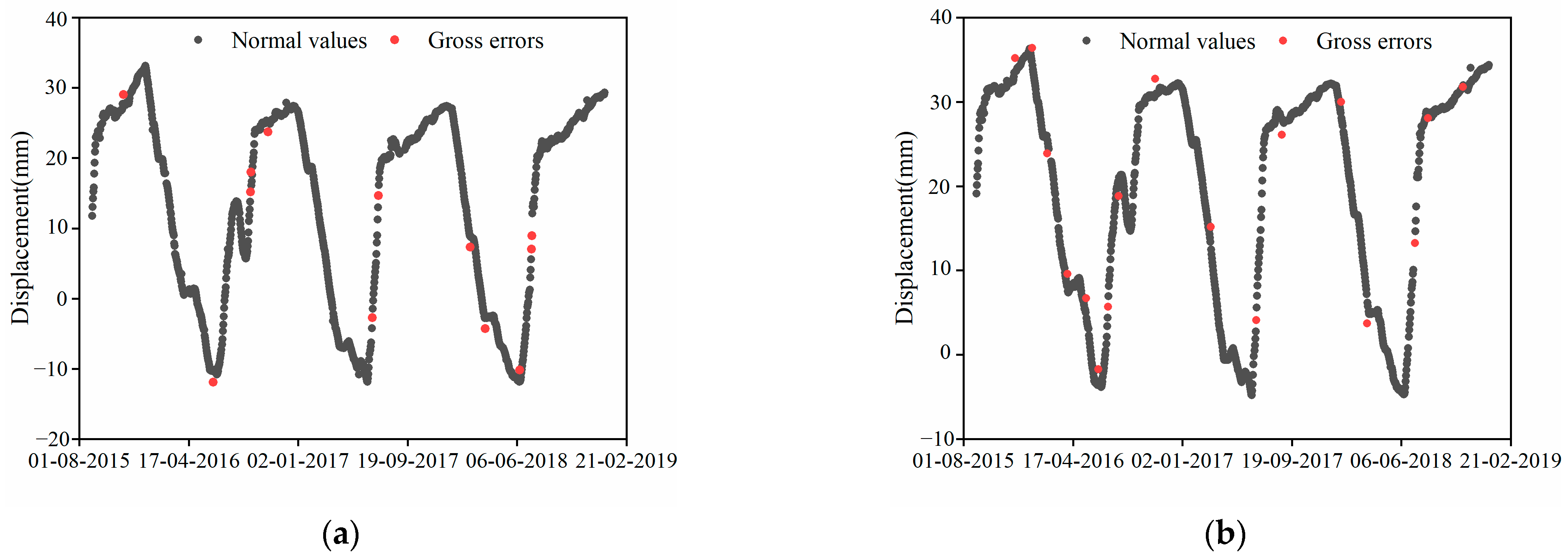
The detection results of the FCM-LOF and FCM-DBSCAN algorithms for monitoring points PL13-1 and PL13-2 in Zone Ⅱ are illustrated in Figure 10 and Figure 11, respectively. Using the FCM-LOF algorithm, LOF values are computed for each data point. Based on the distribution, data points with LOF values exceeding 1.2 for PL13-1 and PL13-2 are identified as gross errors. For PL13-1, 25 gross errors are identified using the FCM-LOF algorithm, of which 14 are intentionally added as anomalous data points. Through comparative analysis between the two monitoring points, four points are not gross errors, resulting in an identification accuracy of 66.67%. For PL13-2, in addition to the 15 intentionally added anomalous data points, seven additional data points are identified as outliers. Upon comparison, there are 4 points that reflect the dam’s operational state, yielding an identification accuracy of 83.33%.
Using the FCM-DBSCAN algorithm, 19 data points for PL13-1 are classified as gross errors, with seven being intentionally added as anomalous values. Upon comparison with PL13-2, seven of these data points are not gross errors, resulting in an identification accuracy of 58.33%. For PL13-2, 24 data points are classified as gross errors, with 14 being intentionally added as anomalous values. Seven of these data points are identified as data reflecting the dam’s operational state, resulting in an identification accuracy of 82.35%.
The same method is applied to the remaining four monitoring points for gross error detection. The specific identification results are detailed in Table 2 and Comparative Figure 12.
Table 2 lists the correct rate of gross error detection for each monitoring point based on the three methods. The average values of the correct rate are 77.70%, 70.21%, and 95.83% based on FCM-LOF, FCM-DBSCAN, and the proposed method, respectively. Specifically, the correct rate of all six monitoring points is between 66.67% (PL13-1) and 83.33% (PL13-2 and PL11-5) based on the FCM-LOF method, between 53.33% (PL11-5) and 82.35% (PL13-2) based on the FCM-DBSCAN method, and between 93.75% (PL13-1, PL13-2, PL16-3, and PL11-5) and 100% (PL13-3 and PL16-5) based on the proposed method. It is evident that the FCM-LOF and FCM-DBSCAN algorithms exhibit a notable occurrence of omission or misjudgment when identifying gross errors. In comparison, this study combines OPTICS with the LOF algorithm and employs secondary discrimination based on the time of occurrence of outliers at similar monitoring points. This approach effectively categorizes anomalous data into gross errors and points reflecting the dam’s operational state, accurately eliminating genuine gross errors. This indicates that the FCM-OPTICS-LOF algorithm possesses the strongest gross error identification capabilities. The proposed method can be applied to the gross error detection of dam monitoring data. In this way, real and reliable monitoring data representing dam health status can be obtained to provide more accurate guidance for dam management and maintenance.

5. Conclusions

To address the issue of gross error identification in the safety monitoring data of dams and further enhance accuracy while reducing misjudgments, this paper considers leveraging the deformation similarity between measurement points to distinguish gross errors from genuine data influenced by environmental factors. We propose a gross error identification method based on FCM deformation zoning, combining the OPTICS algorithm with the LOF algorithm. We validate the proposed method using measured displacement data from a concrete arch dam as an example and draw the following conclusions:
(1)
The FCM-OPTICS-LOF gross error identification method proposed in this study effectively identifies all gross errors within the dataset. And it will not misjudge abrupt data fluctuations induced by changes in environmental variables as gross errors. This presents a reliable and effective new approach for gross error identification in dam deformation monitoring data.
(2)
The proposed FCM-OPTICS-LOF method for gross error identification demonstrates higher accuracy compared to both the standalone LOF method and the widely employed DBSCAN method, belonging to the same density clustering algorithms. This affirms the superiority of the proposed method. Furthermore, the method’s ability to identify gross errors by comparing different measurement points allows simultaneous recognition of two or more points, significantly enhancing the efficiency of gross error detection.
(3)
Although the proposed gross error identification method in this paper achieves accurate identification, the threshold selection of the LOF value needs to be manually judged and determined for the specific situation. How to adaptively select the appropriate threshold needs to be further studied and explored.

Author Contributions

Conceptualization, L.C., C.G. and S.Z.; methodology, L.C., C.G. and Y.W.; software, L.C., C.G. and S.Z.; validation, L.C., C.G. and Y.W.; formal analysis, L.C. and C.G.; investigation, C.G.; resources, S.Z.; data curation, L.C. and S.Z.; writing—original draft preparation, L.C. and S.Z.; writing—review and editing, C.G. and Y.W.; supervision, C.G.; project administration, C.G. and S.Z.; funding acquisition, C.G. All authors have read and agreed to the published version of the manuscript.

Funding

This research was funded by the National Natural Science Foundation of China (Grant Nos. U2243223 and 52209159), the Water Conservancy Science and Technology Project of Jiangsu (Grant No. 2022024), the Fundamental Research Funds for the Central Universities (Grant No. B230201011), the Jiangsu Young Science and Technological Talents Support Project (Grant No. TJ-2022-076), and the China Postdoctoral Science Foundation (2023M730934).

Data Availability Statement

Data are contained within the article.

Conflicts of Interest

The authors declare no conflicts of interests.

Appendix A

Table A1 shows the positions and magnitude of gross errors added to PL13-3 and PL16-3. Table A2 shows the positions and magnitude of gross errors added to PL11-5 and PL16-5. Figure A1 and Figure A2 display the reachable distance plots and LOF scatter plots for PL13-3 and PL16-3 in Zone Ⅰ. Figure A3 and Figure A4 show the reachable distance plots and LOF scatter plots for PL11-5 and PL16-5 in Zone Ⅳ.
Table A1. Locations and magnitudes of gross errors introduced in monitoring points PL13-3 and PL16-3.
PL13-3PL16-3
DataRaw Data/mmGross
Error Size/mm
the Data
after
Adding
the Gross
Error/mm
DataRaw Data/mmGross
Error Size/mm
the Data after Adding the Gross
Error/mm
6 October 201538.87−1.5637.315 November 201534.091.8635.95
24 November 201539.32−1.7837.5420 December 201536.351.7338.08
19 January 201638.721.4540.1725 February 201630.16−1.9528.21
22 March 201622.722.325.0223 April 201621.75−1.620.15
30 May 201613.111.891529 July 201628.71−226.71
22 August 2016281.6829.6818 October 201634.271.5935.86
7 November 201638.52−1.8636.6619 January 201732.23−1.8330.4
14 February 201731.661.9633.6221 April 201715.642.5618.2
16 May 201710.841.8212.6618 July 201733.071.6834.75
14 October 201737.22−1.6535.5726 October 201734.5−331.5
8 January 201837.73−1.7635.9725 December 201735.141.9637.1
30 March 201817.612.8920.52 March 201827.021.8228.84
13 July 201831.91.933.815 May 201817.09−1.4915.6
27 September 201837.722.840.523 August 201835.27237.27
13 December 201840.771.5342.36 November 201836.551.6738.22
Table A2. Locations and magnitudes of gross errors introduced in monitoring points PL11-5 and PL16-5.
PL11-5PL16-5
DataRaw Data/mmGross
Error Size/mm
Data
after
Adding
the Gross
Error/mm
DataRaw Data/mmGross
Error Size/mm
Data after Adding the Gross
Error/mm
22 September 201530.3−1.5328.7730 September 201530.811.7132.52
23 January 201630.21.6931.8924 November 201531.18−1.7929.39
9 April 201624.671.9826.6529 January 201630.651.8432.49
25 June 201621.72−1.7619.969 April 201625.861.8827.74
7 September 201628.652.831.4517 June 201623.11−1.9221.19
22 December 201632.41−1.6430.7728 July 201629.321.7731.09
26 February 201728.241.5829.8213 September 201630.11−2.427.71
20 May 201721.991.6523.6421 October 201631.411.9233.33
14 August 201731.541.7333.2725 December 201631.47−1.8529.62
23 October 201731.74−1.8229.9210 March 201727.611.5829.19
10 January 201831.29−1.6429.6529 June 201727.53−2.0825.45
5 March 201827.232.229.4316 December 201732.141.733.84
16 June 201823.03−1.7421.297 March 201827.95−1.5526.4
3 September 201831.841.8433.6813 June 201823.841.7225.56
5 November 201831.99−2.329.6912 September 201832.36−1.6830.68
Figure A1. (a) Reachability distance for measurement point PL13-3; (b) Reachability distance for measurement point PL16-3.
Water 16 00978 g0a1
Figure A2. (a) LOF values for preliminary gross errors at measurement point PL13-3; (b) LOF values for preliminary gross errors at measurement point PL16-3.
Water 16 00978 g0a2
Figure A3. (a) Reachability distance for measurement point PL11-5; (b) Reachability distance for measurement point PL16-5.
Water 16 00978 g0a3
Figure A4. (a) LOF values for preliminary gross errors at measurement point PL11-5; (b) LOF values for preliminary gross errors at measurement point PL16-5.
Water 16 00978 g0a4

References

  1. Milillo, P.; Perissin, D.; Salzer, J.T.; Lundgren, P.; Lacava, G.; Milillo, G.; Serio, C. Monitoring dam structural health from space: Insights from novel InSAR techniques and multi-parametric modeling applied to the Pertusillo dam Basilicata, Italy. Int. J. Appl. Earth Obs. Geoinf. 2016, 52, 221–229. [Google Scholar] [CrossRef]
  2. Gu, C.; Su, H.; Wang, S. Advances in calculation models and monitoring methods for long-term deformation behavior of concrete dams. J. Hydroelectr. Eng. 2016, 35, 1–14. [Google Scholar]
  3. Yuan, D.; Gu, C.; Gu, H. Displacement behavior analysis and prediction model of concrete gravity dams in cold region. J. Hydraul. Eng. 2022, 53, 733–746. [Google Scholar]
  4. Wu, Z. Safety Monitoring Theory and Its Applications in Hydraulic Structures; Higher Education Press: Beijing, China, 2003. [Google Scholar]
  5. Li, Z.; Hou, H. Dam safety monitoring indices based on motion stability theory. Eng. J. Wuhan Univ. Eng. Ed. 2010, 43, 581. [Google Scholar]
  6. Zhang, C.; Zhou, X.; Gao, C.; Wang, C. On improving the precision of localization with gross error removal. In Proceedings of the 28th International Conference on Distributed Computing Systems Workshops, Beijing, China, 17–20 June 2008; pp. 144–149. [Google Scholar]
  7. Hu, Y.T.; Shao, C.F.; Gu, C.S.; Meng, Z.Z. Concrete Dam Displacement Prediction Based on an ISODATA-GMM Clustering and Random Coefficient Model. Water 2019, 11, 714. [Google Scholar] [CrossRef]
  8. Wang, X.; Wang, Z.-Y.; Wen, K.-L.; Chen, H.-C. The development of Matlab toolbox for gross error in measurement. In Proceedings of the 2011 International Conference on System Science and Engineering, Macau, China, 8–10 June 2011; pp. 461–466. [Google Scholar]
  9. Xiong, Z.; Cui, C.; Pei, D. Research on the Processing of the Gross Error of Shock Wave Overpressure Value. J. Ordnance Equip. Eng. 2021, 42, 94–97. [Google Scholar]
  10. Ge, L.Y.; Wang, Z.Y. Novel uncertainty-evaluation method of virtual instrument small sample size. J. Test. Eval. 2008, 36, 273–279. [Google Scholar]
  11. Zhao, Z.P.; Chen, K.J.; Zhang, H.; Li, Y.; Wu, Z. The method of gross error identification of dam monitoring data based on robust estimation. J. Water Resour. Power 2018, 36, 68–71. [Google Scholar]
  12. Li, X.; Li, Y.L.; Zhang, P.; Yang, Z. Research on an improved Pauta criterion based on M-estimation for gross error identification of monitoring data and its application. China Rural Water Hydropower 2019, 8, 133–136. [Google Scholar]
  13. Qu, X.D.; Yang, J.; Chang, M. A Deep Learning Model for Concrete Dam Deformation Prediction Based on RS-LSTM. J. Sens. 2019, 2019, 4581672. [Google Scholar] [CrossRef]
  14. Al-Samahi, S.S.A.; Ho, K.C.; Islam, N.E. Improving Elliptic/Hyperbolic Localization Under Multipath Environment Using Neural Network for Outlier Detection. In Proceedings of the IEEE Conference on Computer Communications (IEEE INFOCOM), Paris, France, 29 April–2 May 2019; pp. 933–938. [Google Scholar]
  15. Bourquin, J.; Schmidli, H.; van Hoogevest, P.; Leuenberger, H. Pitfalls of artificial neural networks (ANN) modelling technique for data sets containing outlier measurements using a study on mixture properties of a direct compressed dosage form. Eur. J. Pharm. Sci. 1998, 7, 17–28. [Google Scholar] [CrossRef] [PubMed]
  16. Chakravarty, S.; Demirhan, H.; Baser, F. Fuzzy regression functions with a noise cluster and the impact of outliers on mainstream machine learning methods in the regression setting. Appl. Soft Comput. 2020, 96, 106535. [Google Scholar] [CrossRef]
  17. Miao, Y.; Su, H.Y.; Xu, O.G.; Chu, J. Support Vector Regression Approach for Simultaneous Data Reconciliation and Gross Error or Outlier Detection. Ind. Eng. Chem. Res. 2009, 48, 10903–10911. [Google Scholar] [CrossRef]
  18. Ramachandran, V.; Kishorebabu, V. A Tri- State Filter for the Removal of Salt and Pepper Noise in Mammogram Images. J. Med. Syst. 2019, 43, 40. [Google Scholar] [CrossRef] [PubMed]
  19. Mohandoss, D.P.; Shi, Y.; Suo, K. Outlier Prediction Using Random Forest Classifier. In Proceedings of the IEEE 11th Annual Computing and Communication Workshop and Conference (CCWC), Las Vegas, NV, USA, 27–30 January 2021; pp. 27–33. [Google Scholar]
  20. Song, J.T.; Chen, Y.C.; Yang, J. A Novel Outlier Detection Method of Long-Term Dam Monitoring Data Based on SSA-NAR. Wirel. Commun. Mob. Comput. 2022, 2022, 6569367. [Google Scholar] [CrossRef]
  21. Qi, Z.Y.; Sun, F.T.; Mao, Y.P.; Zhou, J.B.; Zhang, C.H.; Li, Q.Y. Research on Gross Error Detecting Method of Monitored Dam Deformation Data Based on Fully Convolutional Networks. Water Resour. Power 2023, 41, 87–90. [Google Scholar]
  22. Wang, L.; Zheng, D. Anomaly Identification of Dam Safety Monitoring Data Based on Convolutional Neural Network. J. Yangtze River Sci. Res. Inst. 2021, 38, 72–77. [Google Scholar]
  23. Hu, J.; Ma, F.H.; Wu, S.H. Anomaly identification of foundation uplift pressures of gravity dams based on DTW and LOF. Struct. Control Health Monit. 2018, 25, e2153. [Google Scholar] [CrossRef]
  24. Song, J.T.; Zhang, S.F.; Tong, F.; Yang, J.; Zeng, Z.Q.; Yuan, S. Outlier Detection Based on Multivariable Panel Data and K-Means Clustering for Dam Deformation Monitoring Data. Adv. Civ. Eng. 2021, 2021, 3739551. [Google Scholar] [CrossRef]
  25. Shao, C.F.; Zheng, S.; Gu, C.S.; Hu, Y.T.; Qin, X.N. A novel outlier detection method for monitoring data in dam engineering. Expert Syst. Appl. 2022, 193, 116476. [Google Scholar] [CrossRef]
  26. Bao, Y.Q.; Tang, Z.Y.; Li, H.; Zhang, Y.F. Computer vision and deep learning-based data anomaly detection method for structural health monitoring. Struct. Health Monit. Int. J. 2019, 18, 401–421. [Google Scholar] [CrossRef]
  27. Harrou, F.; Zeroual, A.; Hittawe, M.M.; Sun, Y. Chapter 6—Recurrent and convolutional neural networks for traffic management. In Road Traffic Modeling and Management; Harrou, F., Zeroual, A., Hittawe, M.M., Sun, Y., Eds.; Elsevier: Amsterdam, The Netherlands, 2022; pp. 197–246. [Google Scholar]
  28. Harrou, F.; Zeroual, A.; Hittawe, M.M.; Sun, Y. Road Traffic Modeling and Management: Using Statistical Monitoring and Deep Learning; Elsevier: Amsterdam, The Netherlands, 2022. [Google Scholar]
  29. Hittawe, M.M.; Langodan, S.; Beya, O.; Hoteit, I.; Knio, O. Efficient SST prediction in the Red Sea using hybrid deep learning-based approach. In Proceedings of the 20th IEEE International Conference on Industrial Informatics (INDIN), Perth, Australia, 25–28 July 2022; pp. 107–114. [Google Scholar]
  30. Zhang, J.; Xie, J.M.; Kou, P.G. Abnormal Diagnosis of Dam Safety Monitoring Data Based on Ensemble Learning. In Proceedings of the 3rd International Workshop on Renewable Energy and Development (IWRED), Guangzhou, China, 8–10 March 2019. [Google Scholar]
  31. Gu, C.S.; Wang, Y.B.; Gu, H.; Hu, Y.T.; Yang, M.; Cao, W.H.; Fang, Z. A Combined Safety Monitoring Model for High Concrete Dams. Appl. Sci. 2022, 12, 12103. [Google Scholar] [CrossRef]
  32. Li, N.; Li, P.; Shi, X.L.; Yan, K.; Ren, W.P. Outlier Identify Based on BP Neural Network in Dam Safety Monitoring. In Proceedings of the 2nd International Asia Conference on Informatics in Control, Automation and Robotics (CAR), Wuhan, China, 6–7 March 2010; pp. 210–214. [Google Scholar]
  33. Liu, J.; Lian, J.J. Outliers Detection of Dam Displacement Monitoring Data Based on Wavelet Transform. In Proceedings of the International Conference on Green Building, Materials and Civil Engineering (GBMCE 2011), Shangri La, China, 22–23 August 2011; pp. 4590–4595. [Google Scholar]
  34. Li, H.J.; Li, J.J.; Kang, F. Risk analysis of dam based on artificial bee colony algorithm with fuzzy c-means clustering. Can. J. Civ. Eng. 2011, 38, 483–492. [Google Scholar] [CrossRef]
  35. Yang, C.; Bao, T. Dam Deformation Prediction Model Based on FCM-XGBoost. J. Yangtze River Sci. Res. Inst. 2021, 38, 66–71. [Google Scholar]
  36. Liu, W.; Chen, B.; Ge, P.; Zhang, X. Deformation prediction model of a high arch dam based on clustering and MO-LSSVR. Adv. Sci. Technol. Water Resour. 2023, 43, 102–108. [Google Scholar]
  37. Li, Z.K.; Li, W.; Ge, W. Weight analysis of influencing factors of dam break risk consequences. Nat. Hazards Earth Syst. Sci. 2018, 18, 3355–3362. [Google Scholar] [CrossRef]
  38. Kumar, K.M.; Reddy, A.R.M. A fast DBSCAN clustering algorithm by accelerating neighbor searching using Groups method. Pattern Recognit. 2016, 58, 39–48. [Google Scholar] [CrossRef]
  39. Kalita, H.K.; Bhattacharyya, D.K.; Kar, A. A new algorithm for Ordering of Points To Identify Clustering Structure Based On Perimeter of Triangle: OPTICS (BOPT). In Proceedings of the 15th International Conference on Advanced Computing and Communications, Indian Inst Technol Guwahati, Guwahati, India, 18–21 December 2007; pp. 523–528. [Google Scholar]
  40. Deng, Z.; Hu, Y.Y.; Zhu, M.; Huang, X.H.; Du, B. A scalable and fast OPTICS for clustering trajectory big data. Clust. Comput. J. Netw. Softw. Tools Appl. 2015, 18, 549–562. [Google Scholar] [CrossRef]
  41. Xiao, X.; Xue, S. An outlier detection algorithm based on improved OPTICS clustering and LOPW. Comput. Eng. Sci. 2019, 41, 885–892. [Google Scholar]
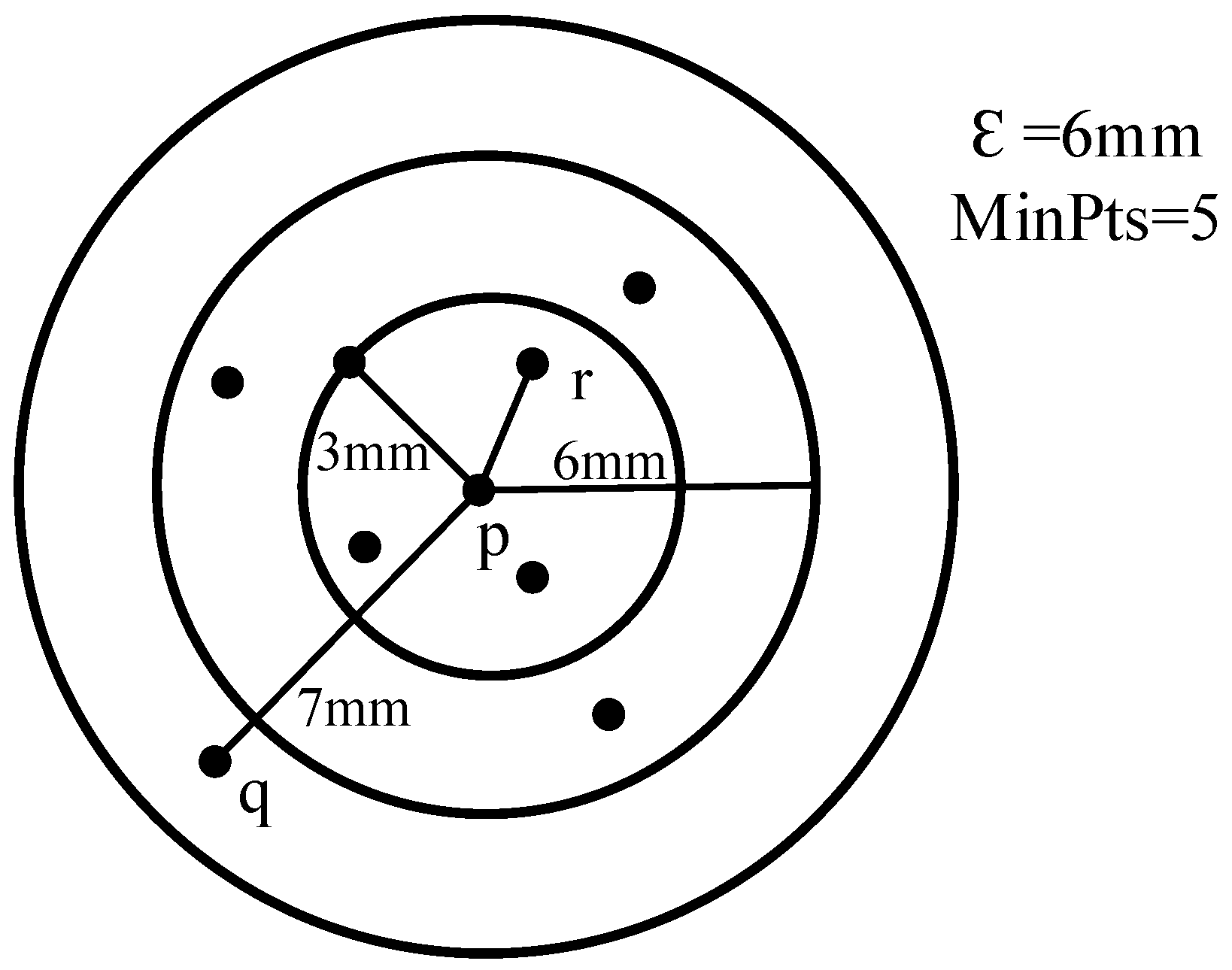
Figure 1. Schematic diagram of the OPTICS algorithm.
Water 16 00978 g001
Figure 2. Schematic diagram of the LOF algorithm for identifying outliers.
Water 16 00978 g002
Figure 3. The flow chart of gross error identification.
Water 16 00978 g003
Figure 4. The photograph of the hyperbolic arch dam.
Water 16 00978 g004
Figure 5. Silhouette coefficients for different numbers of clusters.
Water 16 00978 g005
Figure 6. Clustered zones resulting from deformation monitoring points in the arch dam.
Water 16 00978 g006
Figure 7. Displacement time histories at each measurement point with the inclusion of gross errors: (a) displacement time histories for PL13-1 and PL13-2, (b) displacement time histories for PL13-3 and PL16-3, (c) displacement time histories for PL11-5 and PL16-5.
Water 16 00978 g007
Figure 8. (a) Reachability distance for measurement point PL13-1; (b) Reachability distance for measurement point PL13-2.
Water 16 00978 g008
Figure 9. (a) LOF values for preliminary gross errors at measurement point PL13-1; (b) LOF values for preliminary gross errors at measurement point PL13-2.
Water 16 00978 g009
Figure 10. (a) LOF values for measurement point PL13-1; (b) LOF values for measurement point PL13-2.
Water 16 00978 g010
Figure 11. (a) Gross error identification results for measurement point PL13-1 using FCM-DBSCAN algorithm; (b) Gross error identification results for measurement point PL13-2 using FCM-DBSCAN algorithm.
Water 16 00978 g011
Figure 12. The correct rate of gross error identification using different methods.
Water 16 00978 g012
Table 1. Locations and magnitudes of gross errors introduced in monitoring points PL13-1 and PL13-2.
PL13-1PL13-2
DataRaw Data/mmGross Error Size/mmthe Data after
Adding the Gross Error/mm
DataRaw Data/mmGross Error Size/mmthe Data after Adding the Gross Error/mm
14 November 201527.621.382914 September 201529.34−1.527.84
23 January 201625.15−1.15241 December 201533.511.735.21
31 March 20162.11.43.511 January 201634.591.836.39
14 June 2016−10.5−1.4−11.916 February 201625.76−1.923.86
19 July 20165.781.2274 April 20167.821.769.58
12 September 201615.672.331818 May 20164.726.7
22 October 201625.24−1.5423.716 June 2016−3.391.66−1.73
5 December 201626.71.227.93 August 201620.91−2.118.81
26 March 2017−1.74−1.46−3.229 October 201630.831.8832.71
26 May 2017−9.4−1.40−10.810 March 201712.942.2515.19
11 August 201720.911.5922.526 August 201727.98−1.8926.09
15 February 20188.74−1.447.314 January 201828.361.6530.01
22 March 2018−2.74−1.56−4.317 March 20186.72−33.72
12 June 2018−11.861.66−10.220 July 201824.321.8626.18
19 November 201826.891.3128.218 November 201832.251.7734.02
Table 2. The correct rate of different methods in identifying gross errors.
Monitoring PointsGross Error Identification Method
FCM-OPTICS-LOFFCM-LOFFCM-DBSCAN
PL13-193.75%66.67%58.33%
PL13-293.75%83.33%82.35%
PL13-3100%78.94%75%
PL16-393.75%75%78.94%
PL11-593.75%83.33%53.33%
PL16-5100%78.94%73.33%
Disclaimer/Publisher’s Note: The statements, opinions and data contained in all publications are solely those of the individual author(s) and contributor(s) and not of MDPI and/or the editor(s). MDPI and/or the editor(s) disclaim responsibility for any injury to people or property resulting from any ideas, methods, instructions or products referred to in the content.