Abstract
The current seepage prediction model of the sluice gate is rarely used. To solve the problem, this paper selects the bidirectional long and short-term neural network (BiLSTM) with high information integration and accuracy, which can well understand and capture the temporal pattern and dependency relationship in the sequence and uses the multi-strategy improved Harris Hawks optimization algorithm (MHHO) to analyze its two hyperparameters: By optimizing the number of forward and backward neurons, the overfitting and long-term dependence problems of the neural network are solved, and the convergence rate is accelerated. Based on this, the MHHO-BiLSTM statistical prediction model of sluice seepage is established in this paper. To begin with, the prediction model uses water pressure, rainfall, and aging effects as input data. Afterward, the bidirectional long short-term memory neural network parameters are optimized using the multi-strategy improved Harris Hawks optimization algorithm. Then, the statistical prediction model based on the optimization algorithm proposed in this paper for sluice seepage is proposed. Finally, the seepage data of a sluice and its influencing factors are used for empirical analysis. The calculation and analysis results indicate that the optimization algorithm proposed in this paper can better search the optimal parameters of the bidirectional long short-term memory neural network compared with the original Harris Eagle optimization algorithm, optimizing the bidirectional long short-term memory neural network (HHO-BiLSTM) and the original bidirectional long short-term memory neural network (BiLSTM). Meanwhile, the bidirectional long and short-term neural network (BiLSTM) model shows higher prediction accuracy and robustness.
1. Introduction
The hydraulic industry has a long history of improving human life, ensuring national security, and promoting economic development. Sluice is a common hydraulic engineering, and its main role is to regulate the flow of water. A low-head water retaining structure can be used to generate electricity, control flooding, provide irrigation, or provide water [1], and ensure the rational use of water resources and water environment protection [2]. Once the sluice has an accident, the damage to the traffic and urban infrastructure and the casualties caused by the accident are far more serious than the consequences caused by general public facilities [3]. In the overall safety of sluice, seepage safety occupies an important position. Within the data, it can be seen that many geological disasters and accidents are related to seepage damage [4]. Many sluices have many defects in technology and equipment, which makes the problem of seepage increasingly prominent. It can not only affect the flood protection and flood discharge of the sluice, but also affect the anti-sliding stability of the sluice base and sluice room [5]. The study of seepage problems mainly includes the numerical simulation of seepage, mathematical modeling of seepage, forward and inversion of the seepage field, engineering applications, calculation methods of seepage, quantitative analytical mathematical method, etc. Among them, many researchers have conducted numerical simulations of seepage over the years [6,7], for example, the finite element method, boundary element method, finite analysis method [8], finite integral method, finite difference method, numerical manifold method, and so on, have all been used. Compared with the dam, due to the complexity of the sluice environment, the monitoring data are relatively scarce; at present, the structure behavior analysis experience is very limited. However, the importance of sluices makes their operating state analysis the subject of widespread attention in recent decades.
Since seepage is generally considered a key factor in the design, construction, and safe operation of floodgates, the seepage prediction analysis of floodgates has attracted more and more attention. Since the development of finite element software has accelerated in recent years, many scholars have used different finite element software to simulate, analyze, and calculate seepage flow in hydraulic structure engineering, for example, PLAXIS [9], COMSOL Multiphysics [10,11,12], GeoStudio [13], FLAC3D [14,15], SEEP/W [16], ABAQUS [17,18], FEFLOW [19], FLUENT [20], FLOW3D [21], and so on.
At the same time, the latest development of machine learning also provides a new method for the accurate analysis and prediction of many seepage problems of hydraulic structure projects. To detect abnormal seepage in hydraulic structure engineering in time, it is of great significance to use machine learning methods and historical monitoring data to predict the development trend of seepage characteristics in hydraulic structure engineering. Therefore, seepage prediction models for various hydraulic structures have been proposed and widely used. Hou et al. [22] proposed an integrated multi-target prediction model (MPM) that combines two deep learning methods into a single framework. This model captures both the variation pattern of measurement values with changing load and time, as well as the spatial distribution relationship of these values. Zhao et al. [23] combined the rough set theory (RS) and a long short-term memory network model (LSTM) to develop an RS-LSTM model written in Python by taking advantage of the timeliness of monitoring value changes and the lag of external influences. To optimize XGBoost hyperparameters, Zhang et al. [24] used hybrid Gray Wolf optimization (HGWO), which combines differential evolution (DE) and Gray Wolf optimization (GWO), as well as quad cross-validation, and then used it to predict seepage. Ishfaque et al. [25] built a deep learning model combining recurrent neural networks (RNN) and long short-term memory (LSTM) to predict the seepage degree of hydraulic structure engineering. The influencing factors mainly considered in this method are time series.
Multidimensional inputs present significant challenges to traditional statistical models, deterministic models, mixed models, model adaptive learning, and analyzing complex nonlinear relations. In recent years, neural networks have been widely used in hydraulic structures in deformation prediction [26]. Multilayer neural networks have been widely used in time series forecasting because of their good nonlinear fitting ability. To address the limitation of traditional multilayer neural networks in learning and remembering long-term dependent information, the long short-term memory (LSTM) architecture has been proposed [27]. LSTM neural networks have gained significant popularity and are extensively used in seepage prediction for various hydraulic structures. Compared with the traditional prediction model, it has good prediction performance [28,29]. However, LSTM can only use the previous input information to capture context information, and the dependence on subsequent input is relatively weak. This unidirectional dependency modeling may not capture the temporal patterns and dependencies completely and cannot make full use of the global information in the sequence to solve the gross error problem. For sequences with complex gross errors, the predictive power of LSTM may be limited. Compared with ordinary feedforward neural networks, LSTM is more difficult to train. This may lead to problems such as gradient disappearance or gradient explosion in the process of model training, and it is necessary to use weight initialization techniques and gradient clipping methods to train stability. In recent years, some scholars have optimized LSTM. For example, Girsang A S [30] combined improved Easy Data Augmentation (EDA) with reverse translation methods to improve the macro accuracy and F1 of the BiLSTM model. Based on this, this paper selects a bidirectional long short-term memory neural network (BiLSTM) with stronger context awareness, bidirectional dependent modeling, and stronger gross error solving ability, and adopts a multi-strategy optimization Harris Eagle optimization algorithm (MHHO) with better optimization accuracy and stability to optimize the parameters of this model. This can improve the overfitting and long dependence problems of the BiLSTM model and accelerate the convergence rate of the model.
In conclusion, according to the working characteristics and surrounding environment of the sluice, this paper preliminarily analyzes the possible influencing factors of the seepage of the sluice and selects three influencing factors, namely water pressure, rainfall, and aging, which have a great influence on the seepage of the sluice. As a means of improving accuracy and stability, the parameters of BiLSTM were optimized by using the multi-decision improved Harris Hawks optimization algorithm (MHHO). Therefore, based on the identified main factors, a prediction model for the seepage of slugs is developed according to the BiLSTM of Section 2.2. Then, the MHHO algorithm is used to improve the performance of the BiLSTM model. Section 3 of the paper shows that the model is valid by looking at a case study of sluice engineering in China. A comparison is made between HHO-based models and BiLSTM- and HHO-BiLSTM-based models, and the accuracy and combined prediction effect of this method are verified. Finally, conclusions are drawn in Section 4.
2. Principles of the MHHO-BiLSTM Model
2.1. Statistical Model of Sluice Seepage
The statistical model refers to the regression equation obtained by mathematical statistics based on the cause quantity and the concurrent effect quantity obtained by long-term observation data. It can reflect the change in monitoring effect size and be used in extensional forecasting (including missing measurement interpolation) and operation monitoring [31].
Sluice is a kind of low-head hydraulic structure that uses a sluice gate to hold back and discharge water, and seepage is the main factor that interferes with the sluice structure’s stability. Seepage may cause seepage deformation of the foundation, and serious seepage deformation will cause the foundation to be damaged and even lead to the sluice crashing. The size of the seepage flow reflects the anti-seepage effect of the main body of the sluice, the foundation curtain, and the impermeable parts of the sluice, such as the cover of the sluice, the sheet pile, and the bottom plate, which is an important basis for evaluating the operation safety of the sluice. Rainfall, water levels, and time are the primary factors affecting sluice seepage. The water pressure component, rainfall component, and time effect component are mainly analyzed, and the deformation expression adopted is as follows:
where is the flow of seepage; is the component of water level component; is the component of rainfall; is the component of time; , , , , and are regression coefficients for each component ( = 1, 2); is the adjustment parameter related to the water level weight distribution function, at a fixed observation time , it is a constant; is the adjustment parameter related to rainfall weight distribution function, at a fixed observation time , it is a constant; is the water level’s lag hours of; is the number of hours affected by water level; is the time t’s water level; is the rainfall factor’s lag hours; is the number of hours affected by the rainfall factor; is rainfall factor values at time t extracted by factor analysis; and is divided by 2400, which is the number of hours since the monitoring began until the initial observation began 1.
2.2. BiLSTM
2.2.1. Principles of LSTM
Depending on the length of the time series, the recurrent neural network (RNN) model can be applied. However, when the standard RNN model processes a time series with a long time span, the earliest information will lose its effectiveness along with the model information passing, and the RNN cannot establish long-range structural connections. A vanishing gradient (gradient explosion) problem can be improved by setting hyperparameters, modifying activation functions, dropout pruning, and so on. However, these methods cannot fundamentally solve the problem of gradient disappearance of RNN, so the accuracy improvement effect is poor. In order to solve the problem of long-term dependence of time series, Sepp Hochreiter et al. [27] proposed a long short-term memory network (LSTM) in 1997. It is an important branch of the recurrent neural network model (RNN), which has the advantages of RNN and is improved by adding an internal gate control mechanism to maintain the long-term preservation of information on the basis of RNN. Compared with RNN, LSTM has better performance in long-time series.
LSTM consists of a forgotten gate, input gate, and output gate, and its neuron structure diagram is shown in Figure 1.

Figure 1.
The network structure of LSTM [27].
In Figure 1, from left to right, they are, respectively, the forgetting gate, input gate, cell status update, and output gate.
RNN also exploits sequence dependencies via internal state transfers. It incorporates a gating mechanism to overcome the defects of RNN gradient updates within LSTM. An LSTM gate consists of three parts: forgotten, input, and output, and a state unit coordinates the process.
2.2.2. Principles of BiLSTM
LSTM is used as a basis for the development of BiLSTM, which is a bidirectional long-short-term memory network. LSTM’s learn time series only of past moments, not future moments because cell state is transmitted one-way from front to back. BiLSTM has two unit state conveyor belts, which enables the BiLSTM model to learn the characteristics of future seepage information and perform recursion and feedback on it while using the seepage data information in the past. Therefore, BiLSTM can efficiently utilize the time characteristics of time series and improve the accuracy of model prediction so that the prediction results are more accurate than LSTM.
The BiLSTM network structure is shown in Figure 2.
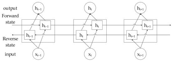
Figure 2.
The network structure of BiLSTM.
Suppose is the time t hidden layer state of the forward LSTM network, which is calculated using the following formula. It can be regarded as a single-layer LSTM network, the process of calculating the state at time t from the state at time t − 1, and is the input at time t.
where is the time t hidden layer state of forward LSTM network; is the LSTM unit; is the t-time input; and is time t − 1 hidden layer state of forward LSTM network.
Similarly, if is time t hidden layer state of the forward LSTM network, its calculation formula is as follows:
where is time t hidden layer state of forward LSTM network; is the LSTM unit; is the t-time input; and is time t − 1 hidden layer state of forward LSTM network.
Combined with hidden layer states and , the BiLSTM network produces a hidden state as its output.
2.3. MHHO Optimizes BiLSTM
2.3.1. MHHO
Harris Hawks Optimization (HHO)
The Harris Hawks Optimization (HHO) is a nature-inspired algorithm proposed by Heidari et al. [32] in 2019, which uses mathematical formulas to simulate the strategies of Harris hawks capturing prey under different mechanisms in reality. The algorithm is divided into two stages of exploration and development, and the transformation is mainly carried out according to the escape energy ; it is used to measure the state of each individual in the group, representing the quality of the individual’s current position. A high escape energy means that an individual is in a not-so-good position, at which time more exploration is needed. Individuals with high escape energies are more likely to explore in a better direction to find a better solution. Its calculation formula is as follows:
where is the initial state of prey energy; is the current iteration count; is the maximum number of iterations; and is the random number between [0, 1].
- (a)
- Exploration phase
When escaping energy , the algorithm enters the exploration phase and performs extensive search operations. The location update formula is as follows:
where is the position of the Harris Hawks on the t + 1 iteration; is the position of the Harris Hawks on the t + 1 iteration; is a randomly selected individual in a population; is the prey location, which is the current best individual; is the current population average position; is the number of individuals in a population; , , , are four independent uniformly distributed random numbers with the values [0, 1]; and and are the lower and upper bounds of the problem, respectively.
- (b)
- Development phase
Case 1: Soft surround. When the escaping energy and , the soft bounding strategy is adopted to update the position; the method is as follows:
where is the jump energy, which is a random number with the value [0, 2], and is the distance between the best individual and the current individual position in the t-th iteration.
Case 2: Hard surround. When the escaping energy and , prey escape failure, surrounded by a hard strategy is adopted to improve the position update at this time, the formula is as follows:
Case 3: Progressive fast dive soft surround. When the escaping energy and , the algorithm is updated by a progressive strategy of rapid dive and soft encircling. If the fitness is not improved after updating with position , position is updated; if the fitness value is not improved, the original position is retained. The specific formula is as follows:
where is the dimension of a problem; is the random vector of size 1 × ; Leavy is the Leavy flight function; and are random numbers that are evenly distributed between (0, 1); is the default constant, set to 1.5; and is the Gamma function.
Case 4: Progressive fast dive hard encircle. When the escaping energy and , the progressive fast dive and hard encircling strategy are adopted to update the position. Currently, the optimal position continues to shrink from the average position for optimization as the population grows. The formula is as follows:
If the fitness is worth improving after the use of position , the position is updated to ; otherwise, the position is used, and the original position is returned if it fails.
Multi-Decision Improved Harris Hawks Optimization Algorithm (MHHO)
While the existing enhancement strategies do enhance the exploration and optimization performance of the HHO algorithm to some extent, they typically only focus on improving specific update strategies or altering the energy reduction method. However, it does not effectively address the issue of global and local optimization blindness. In addition, other optimization algorithms also have their own shortcomings, and many scholars have adopted other optimization algorithms to improve the original algorithm, hoping to achieve better results. For example, Ahmad Sharafati et al. [33] proposed several novel hybrid adaptive neuro-fuzzy inference system (ANFIS) methods called ANFIS-PSO (particle swarm optimization), ANFIS-ACO (ant colony optimization), ANFIS-DE (differential evolution), and ANFIS-GA (genetic algorithm) as predictive models to estimate scour depth downstream of a sluice gate, thereby adopting a new stochastic model based on the integration of Group Method of Data Handling (GMDH) and Generalized Likelihood Uncertainty Estimation (GLUE) to predict scour depth around piers in cohesive soils [34]. This study shows the application of an adaptive neuro-fuzzy inference system (ANFIS) incorporated with particle swarm optimization (ANFIS-PSO), ant colony (ANFIS-ACCO), differential evolution (ANFIS-DE), and genetic algorithm (ANFIS-GA) and assesses the scour depth prediction performance and associated uncertainty in different scour conditions, including live-bed and clear-water [35]. Based on this, to solve the above problems, this paper uses the Multi-Strategy Harris Hawks Optimization algorithm (MHHO) [36], which improves the HHO algorithm from three aspects: Cauchy mutation, random shrinkage exponential function, and adaptive weight. Firstly, the Cauchy distribution function is introduced to improve the global search abilities of the HHO algorithm by mutating the Harris Hawks’ position information. Secondly, the energy-decreasing mechanism is modified by the random contraction index function to effectively adjust the transition. Finally, the HHO algorithm’s local search ability is further improved by introducing a weight factor that is adaptive.
- (a)
- Cauchy variation
Using the HHO optimization, it is difficult to find a local optimum value; by using the Cauchy distribution function, the Harris Hawks algorithm possesses the ability to enhance population diversity, extend the search space, and improve its capacity for global search. In this paper, a global optimal object is optimized by using the Cauchy operator by utilizing both ends of the distribution function. Cauchy distributions can be formulated as follows:
Cauchy’s function peaks at relatively low values. Following the Cauchy mutation, Harris Hawks will spend less time mining the local interval, searching for the global optimum value. Furthermore, the Cauchy function exhibits a gradual decrease from the peak toward both sides. This property becomes significant when updating the position by implementing Cauchy mutations. Harris Hawks have the capability to escape local optima and minimize the presence of local optima constraints. With the Cauchy mutation, the global optimal solution can be obtained, and the optimal solution can be updated using the following formula:
- (b)
- The random shrinking exponential function
In the HHO algorithm, the energy magnitude of the prey, represented by , plays a crucial role in the regulation and transition between global exploration and local exploitation phases. As becomes smaller, the HHO algorithm is more inclined to perform local mining. As becomes larger, the algorithm is more inclined to perform global mining. Nevertheless, the traditional HHO algorithm’s energy equation represents as a linear decrease from its maximum value to the minimum value, which fails to accurately capture the natural process of Harris Hawks hunting prey. Mathematicians simulate the predator-prey interaction and draw the conclusion that the random contraction exponential function is more suitable for expressing the energy change when the prey flees. Therefore, this optimization algorithm proposes to modify the linear decreasing energy regulation mechanism and integrate the random contraction index function into the decreasing process of prey energy , and the corresponding energy equation is as follows:
- (c)
- The adaptive weight
It is important to consider the inertia weighting factor, which determines how much time the algorithm spends on global searches when it is high. The algorithm uses relatively more time for local search when the inertia weighting factor is small, and it is capable of fine-tuning the search for optimal results. The prey position represents the current optimal solution of the HHO algorithm, and the position of the Harris Hawks habitat is inversely guided. Its iterative update directly determines the optimization performance of the algorithm. Therefore, in order to improve the local exploitation ability of the algorithm, it is necessary to re-update the domain of the prey position to find a better solution.
Considering the above, this optimization algorithm introduces an adaptive weight method. During the four hunting mechanisms, when Harris Hawks are searching for prey, the prey adjusts its position using a reduced adaptive weight, enhancing the local optimization capabilities of the algorithm. The adaptive weight formula and prey position update can be expressed as follows:
where is the maximum number of iterations, and is the current iteration count. The integration of the adaptive weighting factor ω enhances the local exploration capabilities of the MHHO algorithm, resulting in an improved ability to mine local optima.
2.3.2. The Establishment Process of the Sluice Seepage Prediction Model Based on MHHO-BiLSTM
The establishment process of the sluice seepage prediction model based on MHHO-BiLSTM is divided into the following steps:
Step 1: Entering the data. Input the original sluice seepage data required for MHHO-BiLSTM model training.
Step 2: Normalization. The normalization method is used to process the data, and the data range is limited between positive and negative 1, which can fix the order of magnitude of the data to improve the training speed and facilitate data analysis.
Step 3: Dividing the normalized processed data into the training set and test set. The data is partitioned with a 70% to 30% ratio, where 70% of the data is allocated for training purposes, and the remaining 30% is reserved as the test set. The training set is trained by the BiLSTM model and continuously back-replaced, and the test set is predicted by the BiLSTM model for the future period of sluice seepage data.
Step 4: Based on the BiLSTM model’s results, the maximum correntropy test is performed to determine if the data meets the requirements.
Step 5: The MHHO algorithm optimizes the parameters. BiLSTM uses the MHHO algorithm to optimize the number of hidden layer nodes, the initial learning rate and the regularization coefficient, and values that are not accurate after iterations are cycled.
Step 6: The maximum correntropy test is carried out again on the calculated data, and the predicted data and test index can be output if the requirements are met. If the requirements are not met, the fifth step is carried out until the optimal solution and fitness value are obtained.
The modeling process of MHHO-BiLSTM is illustrated in Figure 3.

Figure 3.
The modeling process of MHHO-BiLSTM model.
2.4. Evaluation Method for the Effectiveness of the Prediction Model
The effect of time series prediction can be comprehensively considered from two aspects: the subjective level and objective level. Taking a subjective view of the chart, one can see how the predicted experimental data differ from the standard data; that is, the quality of the predicted results can be directly judged by the observation method. However, subjective analysis alone will lack a scientific basis, so it is necessary to supplement objective analysis. From the objective level, we can import the results data of the prediction model into the calculation formula for verification and obtain the numerical error results. In this paper, four types of evaluation indicators are selected, and the calculation formulas of different evaluation indicators are different, as shown in the following formula:
Index 1: Mean Absolute Error (MAE), which reflects the average value of the absolute value of the deviation between the forecast data and the average. It is calculated as follows:
Index 2: Mean Square Error (MSE), which reflects the average value of the square deviation between the predicted data and the measured data. The calculation formula can be written as follows:
Index 3: Root Mean Square Error (RMSE), which is calculated by dividing the predicted data by the measured data and multiplying the ratio of measurements by the number of observations. The calculation formula is given by the following:
Index 4: The coefficient of determination (R-square, R2); this index reflects the ratio relationship between the sum of the squared differences in the real value and the predicted value and the sum of the squared differences in the real value and the mean value. The accuracy of the model is judged according to the value of R2, which ranges from [0, 1]. The closer the value is to 1, the more accurate the model is. The calculation formula is as follows:
3. Case Study
This paper selected Bengbu sluice monitoring data for empirical analysis. The position of its pressure-measuring tube is shown in Figure 4. A total of 72 groups of seepage data from 2021 to 2022 were selected for the model test. Among them, the observed seepage value from January 2021 to June 2022 is the training sample, and the observed seepage value from June 2022 to December 2022 is the test sample (July and August are the local flood seasons, and the rainfall is the maximum in a year. The measured seepage data are introduced into the model as rainfall characteristics).
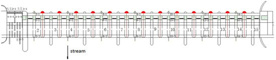
Figure 4.
The position diagram of pressure monitoring pipe in Bengbu Gate 28-hole control gate.
3.1. The Seepage Prediction of Sluice Based on Statistical Model
In this paper, the measured seepage data of a monitoring point in Bengbu Gate in 2022 are used as test samples, and the BiLSTM network model and MHHO-BiLSTM model are, respectively, used to predict, combined with the prediction results of the stepwise regression statistical model, and the relative errors of the three models are compared. The reliability of the MHHO-BiLSTM model established in this paper is verified. The specific seepage measurement results are shown in Table 1.

Table 1.
The analysis table of measured seepage data of Bengbu Gate.
Using stepwise regression fitting, Table 2 presents predicted values and relative errors.
Table 2.
Stepwise regression fitting predicted values and relative errors of monitoring points.
The seepage prediction calculated by the stepwise regression method is shown in Figure 5.

Figure 5.
Seepage prediction diagram calculated by stepwise regression model.
3.2. The BiLSTM Network Model Training and Prediction
The measured seepage value of the No. 2-1 monitoring point on the upstream side of the middle pier on the 2# bottom plate of the Bengbu Gate from January 2021 to June 2022 is used as the training sample. According to the prediction principle of the exponential curve, the LSTM model’s outputs and inputs are the seepage value and influence factor parameters, respectively. Thus, the 10 and 1 nodes are in the input and output layers, respectively. The output item is the No. 2-1 monitoring point on the upstream side of the middle pier of the 2# bottom plate of the Bengbu Gate. The predicted samples are measured seepage values from January 2022 to December 2022 at monitoring points No. 2-1 on the upstream side of the middle pier of the 2# bottom slab of the Bengbu Gate.
Initially, there are 10 nodes in the hidden layer, and those 10 nodes are increased one by one for trial calculations. An evaluation criterion is determined based on the minimum average relative error of the training sample. This paper uses the BiLSTM hidden layer, which, as shown in Figure 2, has a minimum relative error of 4.31% when there are 100 hidden layer nodes. Construction training is conducted with 50 batches and 500 iterations, with a 0.001 target error. Figure 6 describes the number of hidden layer nodes and the training sample average relative error of the curve, and Figure 7 is the process line between the measured seepage value and the fitting value of the LSTM network model at the monitoring point No. 2-1 on the upstream side of the middle pier of the 2# bottom plate.
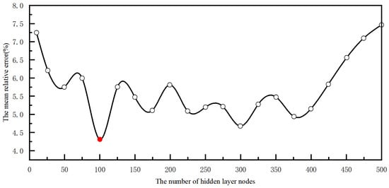
Figure 6.
The number of hidden layer nodes and the training sample average relative error of curve (The white dots are the number of hidden layer nodes, and the red dots are the number of optimal hidden layer nodes).
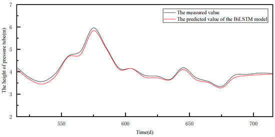
Figure 7.
Process line between measured seepage value and the BiLSTM model fitting value (June 2022~December 2022).
It can be seen from Figure 7 that the fitting value of the BiLSTM network model is consistent with the measured value, and the fitting effect of the model is good, except for several cusps of the curve with relatively large data runout. As can be seen from Table 3, the absolute relative error of the BiLSTM network model in predicting seepage at the No. 2-1 monitoring point on the upstream side of the middle pier of Bengbu Gate 2# bottom floor ranges from 0.35% to 14.96%, and the average absolute value of relative error is 7.41%, indicating a good prediction effect.
Table 3.
Comparison between the predicted results of the BiLSTM model and the measured values.
3.3. The Establishment and Prediction of the MHHO-BiLSTM Model
The utilization of the MHHO optimization algorithm aims to enhance the prediction accuracy of BiLSTM network models even further. Using the fitting values of the BiLSTM network model from June 2022 to December 2022 in Section 3.2, the relative error sequence can be obtained. The subsequent calculation procedures and outcomes are outlined as follows.
The multi-strategy Improved Harris Hawks Optimization Algorithm (MHHO) is used to optimize three parameters (the number of hidden layer nodes, initial learning rate, and regularization coefficient) of BiLSTM. The initial parameters were set as follows: the population number N = 36; the maximum number of iterations T = 500; and the boundary ranges of the three parameters are [1 × 10⁻⁵, 1 × 10⁻²], [0.0001, 0.002], and [10, 100], respectively. Iterative optimization using Harris Hawks with multi-strategy improved methods yields the optimal parameter combination as follows: there are 100 nodes in the hidden layer, the initial learning rate is 0.002, and the regularization coefficient is 1.52 × 10⁻⁵. The convergence curve of MHHO-BiLSTM is shown in Figure 8.
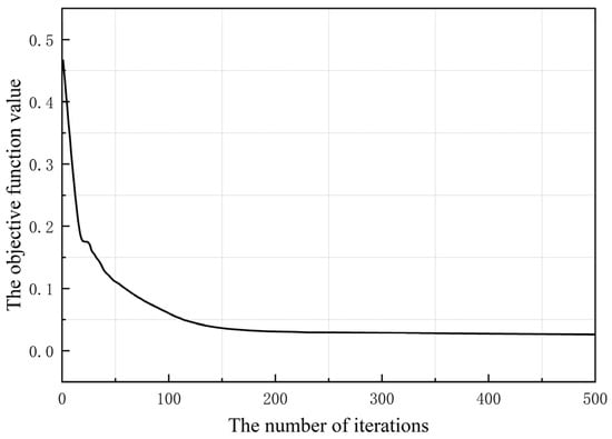
Figure 8.
The convergence of the MHHO-BiLSTM.
In order to further test the effectiveness and superiority of the MHHO-BiLSTM model in sluice seepage prediction, three models, namely MHHO-BiLSTM, BiLSTM, and step-by-step regression, were selected for comparison. In order to compare the prediction effects of MHHO-BiLSTM, BiLSTM, and stepwise regression, the mean absolute error, mean square error, root mean square error, and determination coefficient are taken as the measurement standards, and the evaluation index data of the three models are shown in Table 4. The errors of the test set and the training set are shown in Figure 9 and Figure 10, respectively.
Table 4.
The comparison of evaluation indexes of the three models.
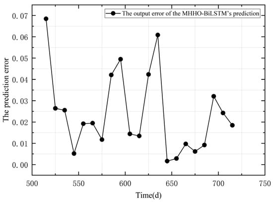
Figure 9.
The prediction error of testing sets.
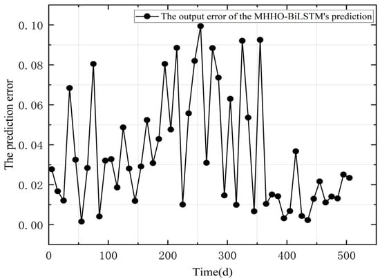
Figure 10.
The prediction error of training sets.
3.4. The Comparison of Model Accuracy
According to the calculation results of seepage flow at the No. 2-1 monitoring point on the upstream side of the middle pier of the 2# bottom plate of the Bengbu Gate in Section 3.2 and Section 3.3, combined with the stepwise regression statistical model’s predictions, the measured values from January 2022 to December 2022 are used to make prediction comparisons. Table 4 and Figure 10 and Figure 11 show the prediction results of the three models, as well as relative errors for each. In Figure 11, the predicted seepage value is compared to the measured value at the pier measurement point; Figure 12 is the absolute relative error of the predicted seepage value at the pier measurement point; Table 5 is the comparison of the relative error of the predicted seepage value at the pier measurement point; M-B model represents the MHHO-BiLSTM model.
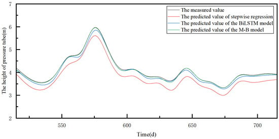
Figure 11.
The measured values of the pier and the predicted seepage values of the three models.
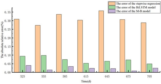
Figure 12.
The relative error absolute values of the three models predicting seepage at the pier monitoring points.
Table 5.
The comparison table of relative errors predicted by three models at the pier monitoring points.
As shown in Figure 11, the measured seepage value at the No. 2-1 monitoring point on the upstream side of the middle pier of floor 2# changes with time non-linearly. In addition, the predicted seepage by the BiLSTM network model and the MHHO-BiLSTM model corresponds to the measured data change trend. In dealing with nonlinear data, the prediction effect of the stepwise regression statistical model is inferior to the BiLSTM network model and MHHO-BiLSTM model. As can be seen from Figure 12 and Table 5, in terms of the relative error of model prediction in the 12 forecasting months, the MHHO-BiLSTM model is the smallest on the whole, while the stepwise regression statistical model is the largest on the whole. Statistically, the stepped-regression model, the BiLSTM network model, and the MHHO-BiLSTM model have mean absolute relative errors of 30.38%, 7.41%, and 1.99%, respectively. It can be seen that the accuracy of the BiLSTM network model is better than the stepped-regression statistical model, and the accuracy of the MHHO-BiLSTM model is better than the BiLSTM network model.
4. Conclusions
Via the main research contents, the following conclusions can be drawn:
- (1)
- According to the results of the main influencing factors of seepage, MHHO was introduced to optimize the BiLSTM model and establish the seepage model of the sluice. The model increases the correlation coefficient R2 from 0.8923 to 0.9942 and decreases the root-mean-square error RMSE from 0.2412 to 0.0530. Compared with the BiLSTM model and stepwise regression model, the R2 value and RMSE value of the predicted results of this method are the largest and the smallest. Case study analysis shows that the MHHO-BiLSTM model has good predictive performance, which indicates the good predictive ability of long-term data series.
- (2)
- The MHHO optimization algorithm can help the BiLSTM model find the optimal parameter combination: the number of forward neurons and the number of backward neurons, so as to improve the performance of the BiLSTM model. The global search capability of the MHHO optimization algorithm can help regulate the complexity of the BiLSTM model to reduce the risk of overfitting, thereby improving the generalization ability of the BiLSTM model on previously unseen data. MHHO optimization algorithm has a strong global search ability, which can help accelerate the convergence process of the BiLSTM model and reduce the training time and calculation cost. MHHO optimization algorithm may help to improve the performance of the BiLSTM model when dealing with long-term dependence and strengthen its modeling ability for long-term dependence by optimizing parameters or model structure.
- (3)
- Sluice seepage problems involve time series data, and BiLSTM is able to consider both the current moment input and the previous and subsequent input information. This enables BiLSTM to more comprehensively capture the time before and after information and timing patterns in the sluice seepage data, which helps to better understand and model the seepage behavior. BiLSTM has strong modeling capabilities and can handle complex nonlinear relationships and timing dependencies. The seepage problem of sluice often involves many influencing factors, and the relationship between these factors may be complicated. BiLSTM is able to build a model and make predictions by learning the temporal patterns in the data. BiLSTM’s bidirectional structure allows the entire time series data to be processed at once. This means that BiLSTM is able to use global information to make predictions rather than just local information at the current moment. For the sluice seepage problem, global dependency modeling is helpful to better understand the correlation and influence of different times in the sluice system. In the seepage problem of the sluice gate, there may be a correlation between several variables, such as temperature, water pressure, aging, and so on. BiLSTM can process multiple input variables at the same time, building predictive models by learning the interactions between them. This gives BiLSTM an advantage in solving multivariable problems.
- (4)
- However, BiLSTM models typically require large amounts of data to be trained in order to effectively capture and learn patterns and trends in time series data. If the amount of data available is small, the BiLSTM model may not be adequately trained, resulting in degraded model performance. These disadvantages should be considered comprehensively according to the specific situation, and the use of the BiLSTM model in predicting the seepage problem of sluice should be weighed. Issues such as the amount of data may need to be fully considered to achieve better predictive performance.
This paper provides a new idea for the seepage prediction of sluice. In addition, the robustness of the MHHO optimization algorithm should be evaluated in more engineering projects and in different scenarios, and it should be extensively validated to verify the applicability and universality of the proposed model.
Author Contributions
Conceptualization, Z.H., C.G. and S.Z.; methodology, Z.H., H.G. and C.S.; software, Z.H., J.P. and C.S.; validation, S.Z. and Y.W.; formal analysis, M.Z.; investigation, H.G.; resources, C.G., J.P. and Y.W.; data curation, Z.H. and C.S.; writing—original draft preparation, Z.H. and S.Z.; writing—review and editing, C.G. and H.G.; supervision, C.G.; project administration, C.G., H.G., J.P., Y.W. and M.Z.; funding acquisition, C.G., J.P., Y.W., H.G. and C.S. All authors have read and agreed to the published version of the manuscript.
Funding
This research was funded by the National Natural Science Foundation of China (Grant Nos. U2243223 and 52209159), the Fundamental Research Funds for the Central Universities (Grant No. B230201011), the Anhui Provincial Natural Science Foundation “Water Sciences” Joint Fund (2208085US17), the Jiangsu Young Science and Technological Talents Support Project (Grant No. TJ-2022-076), the Fund of Water Conservancy Technology of Xinjiang Province (XSKJ-2023-23), the Water Conservancy Science and Technology Project of Jiangsu (Grant No. 2022024), and the China Postdoctoral Science Foundation (2023M730934).
Data Availability Statement
Restrictions apply to the availability of these data. Data was obtained from the Anhui Provincial Natural Science Foundation “Water Sciences” Joint Fund and are available from the author with the permission of the Anhui Provincial Natural Science Foundation “Water Sciences” Joint Fund.
Conflicts of Interest
The authors declare no conflicts of interest.
References
- Fan, X.; Wu, Z.; Liu, L.; Wen, Y.; Yu, S.; Zhao, Z.; Li, Z. Analysis of Sluice Foundation Seepage Using Monitoring Data and Numerical Simulation. Adv. Civ. Eng. 2019, 2019, 2850916. [Google Scholar] [CrossRef]
- Hong, P.; Cao, B.; Ai, D. Based on the exploration of sluice engineering construction technology in hydraulic engineering. In Proceedings of the Guangzhou Sub-Forum of 2023 Smart City Construction Forum, Guangzhou, China, 26 March 2023. (In Chinese). [Google Scholar]
- Zhou, W. Safety Problems and treatment measures of sluice operation. Sci. Life 2012, 186. (In Chinese) [Google Scholar]
- Li, H. Study on Seepage Flow of the Sluice Foundation Based on AutoBANK Software. Master’s Thesis, Ocean University of China, Qingdao, China, 2015. (In Chinese). [Google Scholar]
- Zhao, Y.; Cai, T.; Li, J.; Gou, J. Study on seepage problem of sluice. Dwelling 2019, 1, 157. (In Chinese) [Google Scholar]
- Zhou, X.; Gu, X.; Yu, M.; Qian, Q. Seismic bearing capacity of shallow foundations resting on rock masses subjected to seismic loads. KSCE J. Civ. Eng. 2016, 20, 216–228. [Google Scholar] [CrossRef]
- Yue, N.; Zhang, D.; Chen, J.; Song, P.; Wang, S.; Qiu, S.; Su, G.H.; Zhang, Y. The development and validation of the inter-wrapper flow model in sodium-cooled fast reactors. Prog. Nucl. Energy 2018, 108, 54–65. [Google Scholar] [CrossRef]
- Pokharel, G.; Honjo, Y. Mapped infinite elements in multilayered seepage analysis. In Computer Methods and Advances in Geomechanics; Balkma: Rotterdam, The Netherlands, 1994; pp. 1243–1248. [Google Scholar]
- Pongsivasathit, S.; Petchgate, W.; Horpibulsuk, S.; Piyaphipat, S. Composite contiguous pile wall and deep mixing column wall as a dam—Design, construction and performance. Case Stud. Constr. Mater. 2022, 16, e00904. [Google Scholar] [CrossRef]
- Zhang, K.; Xu, L.; Qiu, L.; Tan, J.; Yang, C.; Zhang, K. Numerical Analysis of Concrete Gravity Dam Seepage Characteristics Evolution considering the Calcium Leaching Effect. Adv. Civ. Eng. 2021, 2021, 9042863. [Google Scholar] [CrossRef]
- Jia, Y.; Ding, Y.; Wang, X.; Zhang, J.; Chen, X. A Numerical Analysis of the Leakage Characteristics of an Embankment Dam Slope with Internal Erosion. Front. Earth Sci. 2022, 10, 866238. [Google Scholar] [CrossRef]
- Wang, R.; Zhu, Y. Finite element analysis of seepage of earth-rock dams in dry and rainy seasons. IOP Conf. Ser. Earth Environ. Sci. 2019, 344, 012112. [Google Scholar] [CrossRef]
- Sun, Y.; Li, Z.; Yang, K.; Wang, G.; Hu, R. Analysis of the Influence of Water Level Change on the Seepage Field and Stability of a Slope Based on a Numerical Simulation Method. Water 2023, 15, 216. [Google Scholar] [CrossRef]
- Zhang, M.; Yao, D.; Lu, H.; Wang, H. Solution of seepage field in different soil layers of concrete dam foundation by flow net method. IOP Conf. Ser. Earth Environ. Sci. 2020, 546, 052053. [Google Scholar] [CrossRef]
- Bensmaine, A.; Benmebarek, N.; Bensmebarek, S. Numerical Analysis of Seepage Failure Modes of Sandy Soils within a Cylindrical Cofferdam. Civ. Eng. J. 2022, 8, 1388–1405. [Google Scholar] [CrossRef]
- Norouzi, R.; Salmasi, F.; Arvanaghi, H. Uplift pressure and hydraulic gradient in Sabalan Dam. Appl. Water Sci. 2020, 10, 111. [Google Scholar] [CrossRef]
- Chen, Q.; Zhang, P.; Ding, H.; Cong, H.; Yun, L. Study on Seepage Characteristics of Composite Bucket Foundation under Eccentric Load. China Ocean. Eng. 2021, 35, 123–134. [Google Scholar] [CrossRef]
- Liu, B.; Li, J.; Liu, Q.; Liu, X. Analysis of Damage and Permeability Evolution for Mudstone Material under Coupled Stress-Seepage. Materials 2020, 13, 3755. [Google Scholar] [CrossRef] [PubMed]
- Guo, Q.; Huang, J. Analysis of the influence of the interlayer staggered zone in the basalt of Jinsha River Basin on the main buildings. IOP Conf. Ser. Earth Environ. Sci. 2018, 113, 012099. [Google Scholar] [CrossRef]
- Bai, L.; Che, W.; Wang, S. Study on the Influence of Groundwater Seepage on the form of the Layout of Soil Source Heat Pump. Procedia Eng. 2016, 146, 445–449. [Google Scholar] [CrossRef][Green Version]
- Safari Ghaleh, R.; Aminoroayaie Yamini, O.; Mousavi, S.H.; Kavianpour, M.R. Numerical Modeling of Failure Mechanisms in Articulated Concrete Block Mattress as a Sustainable Coastal Protection Structure. Sustainability 2021, 13, 12794. [Google Scholar] [CrossRef]
- Hou, W.; Wen, Y.; Deng, G.; Zhang, Y.; Wang, X. A multi-target prediction model for dam seepage field. Front. Earth Sci. 2023, 11, 1156114. [Google Scholar] [CrossRef]
- Zhao, M.; Jiang, H.; Chen, S.; Bie, Y. Prediction of Seepage Pressure Based on Memory Cells and Significance Analysis of Influencing Factors. Complexity 2021, 2021, 5576148. [Google Scholar] [CrossRef]
- Zhang, K.; Gu, C.; Zhu, Y.; Chen, S.; Dai, B.; Li, Y.; Shu, X. A Novel Seepage Behavior Prediction and Lag Process Identification Method for Concrete Dams Using HGWO-XGBoost Model. IEEE Access 2021, 9, 23311–23325. [Google Scholar] [CrossRef]
- Ishfaque, M.; Dai, Q.; Haq, N.U.; Jadoon, K.; Shahzad, S.M.; Janjuhah, H.T. Use of Recurrent Neural Network with Long Short-Term Memory for Seepage Prediction at Tarbela Dam, KP, Pakistan. Energies 2022, 15, 3123. [Google Scholar] [CrossRef]
- Zheng, S.; Gu, C.; Shao, C.; Hu, Y.; Xu, Y.; Huang, X. A Novel Prediction Model for Seawall Deformation Based on CPSO-WNN-LSTM. Mathematics 2023, 11, 3752. [Google Scholar] [CrossRef]
- Hochreiter, S.; Schmidhuber, J. Long short-term memory. Neural Comput. 1997, 9, 1735–1780. [Google Scholar] [CrossRef] [PubMed]
- Hu, Y.; Gu, C.; Meng, Z.; Shao, C.; Min, Z. Prediction for the Settlement of Concrete Face Rockfill Dams Using Optimized LSTM Model via Correlated Monitoring Data. Water 2022, 14, 2157. [Google Scholar] [CrossRef]
- Bolboacă, R.; Haller, P. Performance Analysis of Long Short-Term Memory Predictive Neural Networks on Time Series Data. Mathematics 2023, 11, 1432. [Google Scholar] [CrossRef]
- Girsang, A.S. Modified EDA and backtranslation augmentation in deep learning models for Indonesian aspect-based sentiment analysis. Emerg. Sci. J. 2022, 7, 256–272. [Google Scholar]
- Sheng, J.; Liu, J.; Li, J. Statistical mathematical model of seepage flow in earth-rock dam. Sci. Res. Water Conserv. Water Transp. 1995, 4, 435–443. (In Chinese) [Google Scholar]
- Heidari, A.A.; Mirjalili, S.; Faris, H.; Aljarah, I.; Mafarja, M.; Chen, H. Harris hawks optimization: Algorithm and applications. Futur. Gener. Comput. Syst. 2019, 97, 849–872. [Google Scholar] [CrossRef]
- Sharafati, A.; Tafarojnoruz, A.; Shourian, M.; Yaseen, Z.M. Simulation of the depth scouring downstream sluice gate: The validation of newly developed data-intelligent models. J. Hydro-Environ. Res. 2019, 29, 20–30. [Google Scholar] [CrossRef]
- Sharafati, A.; Tafarojnoruz, A.; Yaseen, Z.M. New stochastic modeling strategy on the prediction enhancement of pier scour depth in cohesive bed materials. J. Hydroinform. 2020, 22, 457–472. [Google Scholar] [CrossRef]
- Sharafati, A.; Tafarojnoruz, A.; Motta, D.; Yaseen, Z.M. Application of nature-inspired optimization algorithms to ANFIS model to predict wave-induced scour depth around pipelines. J. Hydroinform. 2020, 22, 1425–1451. [Google Scholar] [CrossRef]
- Guo, Y.; Liu, S.; Gao, W.; Zhang, L. Improved harris hawks optimization algorithm with multiple strategies. Microelectron. Comput. 2021, 38, 18–24. (In Chinese) [Google Scholar]


Disclaimer/Publisher’s Note: The statements, opinions and data contained in all publications are solely those of the individual author(s) and contributor(s) and not of MDPI and/or the editor(s). MDPI and/or the editor(s) disclaim responsibility for any injury to people or property resulting from any ideas, methods, instructions or products referred to in the content. |
© 2024 by the authors. Licensee MDPI, Basel, Switzerland. This article is an open access article distributed under the terms and conditions of the Creative Commons Attribution (CC BY) license (https://creativecommons.org/licenses/by/4.0/).