Abstract
In this study, we aimed to verify the two relationships on large wood export, as follows: (1) the relationship between large wood recruitment and landslides triggered by intense rainfalls and (2) the relationship between large wood export and the long-term large wood budget on an annual scale, based on the direct export of large wood caused by an increase in large wood recruitment with extreme rainfall events, as well as the baseflow of large wood, which is mainly old large wood recruitment stored at the slopes and in the stream. To reproduce these two relationships, the model consisted of two frameworks, as follows: (1) the rainfall-induced analytical shallow landslide model, with 30 m spatial resolution for large wood recruitment and (2) the double/triple storage function, with the lumped hydrological method at a watershed scale for large wood entrainment. Application of the model to 212 dam reservoir watersheds across Japan resulted in reproducibility in the estimation of large wood export volumes in 134 of the target dam reservoir watersheds, which contribute 63.2% of the target basins. This indicated that our results verified these two relationships as primary relationships. To analyse the difference in large wood export systems, a frequency analysis was conducted using correlation analysis based on large wood export volume and the cumulative values of six patterns of large wood recruitment volumes. The results indicated that there might be differences in large wood export systems between the watersheds represented by the double storage function model and those represented by the triple storage function model.
1. Introduction
1.1. Research Background
Large wood (LW) in rivers has been of growing interest among scientists who have recognised its importance as a functional component of fluvial ecosystems, in the same manner as both sediment and riparian vegetation [1]. LW has a significant impact on river morphology and sediment dynamics [2,3] and provides various positive effects on the aquatic and forest ecosystem [4,5]. Moreover, deadwood is a significant store of carbon and nitrogen and, therefore, plays a central role in their cycle [6,7,8,9,10,11]. LW, like sediment, remains relatively stable, most of the time, in watersheds (Figure 1), where only small, loose pieces of LW can move. However, during large floods, which occur infrequently, large amounts of LW may be transported [12,13], causing potential hazards to human populations and infrastructure [14,15]. The deposition of LW at critical locations (e.g., bridges) may reduce the cross-sectional area of the river channel and cause a reduction in discharge capacity [16,17], resulting in more frequent flooding (Figure 2). This may be accompanied by other processes such as erosion of the river bed, channel avulsion, and localised scouring. Understanding how, where, and why wood moves is therefore fundamental to interpreting and predicting how wood accumulates in watershed systems. The potential flood damage caused by LW necessitates the management of LW; although, in many areas, there are no clear guidelines on how to manage LW. Overall, there is a need for an integrated approach for large-scale LW management along the whole riverine continuum, such as on a watershed scale, rather than site-specific responses to local problems generated by network-wide dynamics. Thus, quantifying the volume of LW is key to studying the role of LW in watersheds.
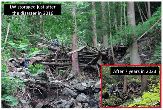
Figure 1.
Field survey of landslide disaster (in both 2016 and 2023) with LW at the Omoto River Basin due to the 2016 rainstorms. Some stored LW after seven years had decayed and re-greened, but the stored capacity had not changed.
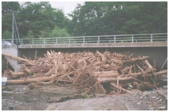
Figure 2.
The deposition of LW at bridges due to Typhoon Etau, which hit Hokkaido in 2003. (Source: the website of the Ministry of Land, Infrastructure, Transport and Tourism).
In Japan, about three-quarters of the country’s area is mountainous and most of it is covered by forests. Therefore, when landslides and flooding occur in the upper reaches of rivers, LW is largely recruited together with sediment. In addition, heavy rainstorm disasters have become more frequent in recent years due to climate change and it is feared that the number of landslides will increase in the future, resulting in an increasing tendency of LW recruitment. The average number of landslides during the 10 years from 2000 to 2009 was 1006 per year, whereas, during the 10 years from 2010 to 2019, the number of landslides increased 1.4 times, to 1476 per year [18]. The importance of taking appropriate measures against landslides involving LW has increased in recent years.
1.2. Recruitment and Entrainment Processes of LW in Streams and Rivers
Numerous studies have reported that the recruitment and entrainment processes of LW in streams and rivers, including the accumulation of LW in forests [19], are caused by various factors such as landslides or flooding, either during or after tropical cyclones or heavy rainstorms [1]. For example, Chen et al. (2013) investigated the LW export downstream after Typhoon Morakot in the Gaoshan and Qijiawan Creeks, located in the Qijiawan catchment in central Taiwan [20]. They found that about 11% of the total LW caused by Typhoon Morakot was exported downstream. Steeb et al. (2017) reported that more than 69,000 m3 of LW was transported by the extreme flood events that occurred in Switzerland in August 2005 [21]. Rickli et al. (2018) reported that LW was deposited both in-channel and on the banks at the 10 headwater rivers in Switzerland from 2004 to 2006 [22]. In Japan, when Typhoon Etau hit Hokkaido in 2003, approximately 50,000 m3 of LW was recruited by landslides and exported into the Nibutani Dam [23]. Landslides, bank instability, debris flows, and fluvial processes are, therefore, potential sources and major transmitters of LW [24,25].
Based on the results of previous studies on LW recruitment, several researchers have proposed methods to estimate LW recruitment from fallen trees in the river channel. Sickle and Gregory (1990) developed a model of LW recruitment to the river using stand density, probability of a single tree falling, and direction of fall [26]. Mazzorana (2009) created hazard index maps of LW recruitment and transport in a watershed by combining the probability of a single tree falling with debris flows, overbank sedimentation, and land use maps [27]. These maps allow the identification of five individual zones for LW recruitment, as follows: the stream influence zone, active wood buffer, recharging wood buffer, preferential recruitment paths, and preferential contributing area. Subsequently, Ruiz-Villanueva and Diez-Herrero et al. (2014) proposed a method to estimate the increase in LW due to landslides, bank erosion, and flooding based on a multi-objective assessment tool using fuzzy logic principles based on the geographic information system [25]. More recently, Scheip and Wegmann (2021) used relative differences in the Normalised Difference Vegetation Index (NDVI) to identify areas on the landscape where vegetation has been removed after natural hazards [28]. Phakdimek and Komori et al. (2023) combined both optical and SAR images for detecting landslide scars, using a classification and regression tree [29].
In Japan, the agencies responsible for local reservoir management are monitoring the total annual LW exported to the reservoirs. In this data set, Seo et al. (2015) proposed that the dynamics of LW in the stream are influenced both directly and indirectly by precipitation patterns [30]. Moreover, Seo and Nakamura (2009) and Seo et al. (2015) proposed that large pieces of LW are directly recruited into channels from surrounding hillslopes in Japan via hillslope processes such as landslides [30,31]. This agrees well with the observational data after heavy storms pass through the affected areas. Chaithong and Komori et al. (2018), based on field studies of heavy rainfall events in the north-eastern part of Japan, reported that landslides disturbed tree roots, causing trees to topple [32]. Fallen trees become LW; some of this LW remains on the hillslope, while some of it is entrained by debris flows, landslides, or flash floods that flow downstream through the watershed (Figure 3). Subsequently, Chaithong and Komori et al. (2018) correctly estimated LW recruitment using the global-scale tree density map [33] and an analytical shallow landslide model, which is coupled with a hillslope hydrological model and driven only by rainfall with 30 m resolution [34], with only approximately 9.1% underestimation [13]. Therefore, it was confirmed that shallow landslides play an important role in LW recruitment and supply a certain amount of LW to streams. Furthermore, debris flows play an important role in transporting LW from upstream to downstream or from small to large river channels. However, few studies have estimated LW recruitment using analytical landslide models.
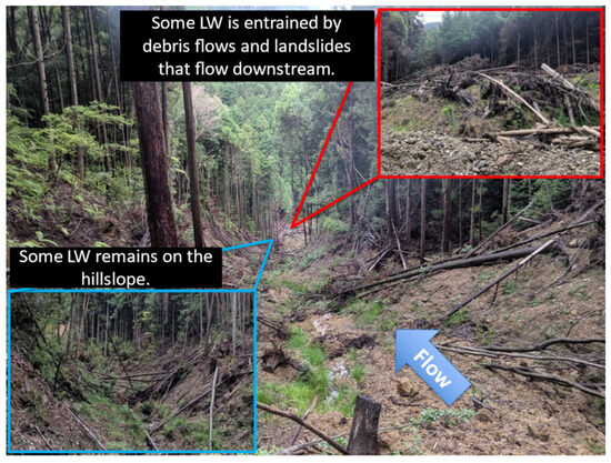
Figure 3.
Field survey of landslide disaster with large wood at the Nomura Dam reservoir watershed in the Hiji River Basin due to the 2018 West Japan rainstorms.
1.3. Quantitative Modelling of LW-Related Processes in an Integrated Approach
As mentioned above, many researchers have studied the role of LW in watersheds; however, to date, there have been far fewer researchers to understand, quantify, and model LW-related processes in an integrated approach. Ruiz-Villanueva et al. (2016) summarised, based on Martin and Benda (2001) [35], that LW dynamics can be considered from the following two perspectives: the mass balance approach and the transport mechanism perspective (Figure 4) [1]. The first perspective can be understood as an LW cycle, similar to the hydrological cycle and equivalent to the floodplain LW cycle [36]. In other words, it is the linkages and feedback associated with the main processes (i.e., recruitment, transport, and storage) that govern the dynamics and mass balance of LW in fluvial systems. The main issues related to LW dynamics from the perspective of the mass balance approach concern the LW balance and LW fluxes, or LW ‘export’ (i.e., how much LW would be transported from upstream to downstream), and their complexity through space and time. The second perspective concerns LW dynamics or the physical factors controlling LW entrainment and transport processes. The questions to be answered in this second perspective are related to hydraulics and fluid mechanics.
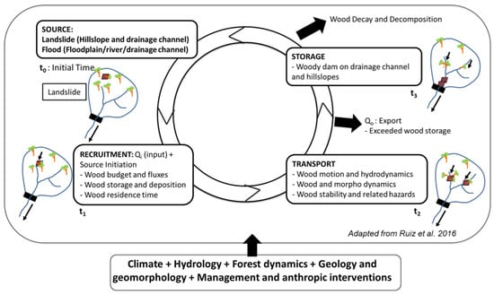
Figure 4.
The dynamics of LW in a forested river watershed are illustrated as a cycle, in which LW recruitment from wood sources might be transported and/or stored (adapted from Ruiz-Villanueva et al. (2016)) [1]. The nonlinearity of these processes is shown as t0–t3, with steady and episodic disturbances potentially triggering recruitment and transport. The time between the processes (t0–t3) may vary among different watersheds and this defines the residence time of LW in the system.
Due to the difficulties in observing changes in LW storage, far fewer studies have addressed the temporal variability in an integrated approach. Boivin et al. (2017) estimated a basin-wide LW budget for the Saint Jean River in Quebec, Canada, based on aerial photographs and field surveys, and found that anthropogenic factors and climate change have a significant impact on LW export [37]. Mazzorana et al. (2011) and Zischg et al. (2018) estimated the amount and location of LW storage originating from riparian forests during river flooding by modelling the physical dynamics of LW export during a single flood event for Swiss rivers [38,39]. Benda and Sias (2003) developed a set of general quantitative expressions based on over 20 years of research on LW that has identified the key variables and their parameter values for the Pacific Northwest [40]. LW budgets were estimated over 100 years, based on LW recruitment, changes in storage, and then inverse analysis of LW export or flux. Hassan et al. (2016) also simulated LW budgets in two mountain streams by modelling a reach-scale LW budget for 100 years using a similar approach to Benda and Sias (2003) [41]. LW loss through decay and downstream transport and loss through depletion was described by a single nonlinear storage function with a lumped model at each reach. However, these studies did not directly use precipitation and fewer studies have specifically documented how precipitation and its varying regimes control the distribution and export pattern of LW. In addition, while post-flood distribution has been occasionally recorded [42], there is no information about the total amount of LW that is transported by very large storms.
Against these research backgrounds, the authors proposed a quantitative model for analysing the mass balance of LW and its export on an annual scale, at a watershed scale (LW-Budget) [43]. LW-Budget consists of the following two frameworks: (1) the rainfall-induced analytical shallow landslide model, with 30 m spatial resolution [34] for the LW recruitment and (2) the double storage function, with the lumped hydrological method at a watershed scale for the LW entrainment (Figure 5). LW-Budget was used to re-analyse 20 years of actual LW export at five dam reservoir watersheds of the Kitakami River catchment, located in the north-eastern part of Japan, and demonstrated that landslide or slope failures are significant procedures of LW export and that the characteristics of LW export can be defined by two relationships; these are the direct export of LW caused by an increase in LW recruitment with the extreme rainfall event, and the baseflow of LW, which is mainly old LW recruitment stored at the slopes and in the stream. To date, such an integrated approach to understanding, quantifying, and modelling LW processes considering the direct impact of precipitation has not been studied and understanding the volume and dynamics of LW can help to predict and prevent the hazards posed by such debris. However, the failure to reproduce the model in one of the five dam reservoir watersheds suggested that there may be different characteristics of LW export from those reproduced by the model at that watershed.
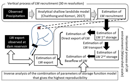
Figure 5.
A schematic diagram of LW-Budget [34,43].
1.4. Approach of This Study
In this study, we aim to verify the generality of hypotheses proposed by the authors on the relationship between LW recruitment and landslides triggered by intense rainfalls, as well as LW export and the long-term LW budget on an annual scale [43], applying LW-Budget to 212 dam reservoir watersheds across Japan. Furthermore, we improve the LW-Budget, which is combined with double and triple storage functions with the lumped hydrological method at a watershed scale for the LW entrainment, to examine the several characteristics of LW exports. The objective is to produce a new, integrated approach to large-scale LW management based on the long-term LW balance and the characteristics of LW export at the watershed scale.
2. Materials and Methods
2.1. Study Sites
In Japan, there are 297 dam reservoir watersheds where agencies responsible for local reservoir management have been monitoring the total annual LW transported to the reservoir. The study sites are 212 dam reservoir watersheds across Japan (Figure 6 and Table 1) selected from among the 297 dam reservoir watersheds according to the following requirements:
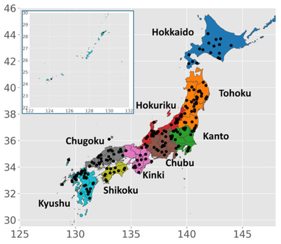
Figure 6.
Distribution of study sites.

Table 1.
The number of dam reservoir watersheds with observed values and dam reservoir watersheds extracted by regions.
- Where the total annual LW transported to the reservoir has been monitored over 10 years.
- Where a substantial total annual LW was observed more than once during the monitoring period.
The interquartile range method of identifying outliers was utilized to determine the presence or absence of a substantial total annual volume of LW. Firstly, the interquartile range is calculated using the runoff volume data for each dam reservoir watershed. Secondly, as a calculation of the threshold of a substantial total annual LW, it is calculated as the third quartile plus the interquartile range multiplied by 1.5. Finally, only dam reservoir watersheds with observed runoff volumes above the threshold in each were selected.
2.2. Estimation of LW Recruitment
The LW-Budget utilized the analytical shallow landslide model [34] to estimate annual LW recruitment into the stream channel with the volume per piece of downed LW, tree density, and the width of the active stream channel [43]. In this study, we enhanced this model by incorporating groundwater and infiltration depth parameters based on Phakdimek et al. (2022) [44]. This model operates as a distributed model, simulating the physical process of slope destabilization induced by an increase in groundwater.
2.2.1. Groundwater and Infiltration Depth in Surface Soil Analysis
Phakdimek et al. (2022) adopted the calculation of groundwater depth (h) proposed by Rosso’s approach [45] into the analytical shallow landslide model [34]. This calculation is calculated under the assumption that evapotranspiration and deep drainage into the bedrock are neglected.
where is the upslope contributing area, is precipitation, is groundwater flow rate, is the volume of water storage, and e is the void ratio of soil. is the saturation of soil, h is groundwater table, is time, is soil depth, and is overland flow discharge occurring when the soil is saturated.
The calculation of groundwater flow rate () was proposed by Darcy’s law. It is expressed in the following equation:
where b is the width, is the slope angle, and is soil permeability. From integrating (1) and (2), derived to (3), the initial condition of stable piezometric at a depth of hi(0) = hi and initial groundwater depth is 0. The cumulative groundwater depth was calculated based on precipitation during rainfall events, with t representing the time elapsed since the start of the rainfall event. Therefore, groundwater accumulates over time and the cumulative groundwater after these events is utilized in the slope stability model. This is expressed in the following equation:
where denotes the hydraulic transmissivity and is the soil depth.
2.2.2. Slope Stability Analysis
The stability of shallow landslides was incorporated into the physically based model, deriving from the infinite slope model. In this model, the failure plane is parallel to the surface of the slope, and the depth of the failure plane is relatively shallow, typically ranging from 0.5 to 3.0 m. Slope stability is commonly described in terms of the factor of safety (), defined as the ratio of the resisting force to the driving force on the failure plane, as expressed below:
where is the effective cohesion of the soil, is the saturated soil density, is the total soil density, is water density, is soil buoyant density, h is the groundwater depth above the failure plane, and is the effective friction angle. For unstable stability, is less than 1.0, which causes landslides, whereas is higher than 1.0 for slope stability.
2.2.3. Estimation of the Annual Volume of LW Recruitment
For the shallow landslide model, elevation data were sourced from the Fundamental Geospatial Data of Japan. Slope angles were computed using the Spatial Analyst Tool in ArcGIS, based on the elevation data. The effective cohesion of soil and the effective friction angle were acquired from the literature review [46] for each soil classification USDA. Other soil parameters were calculated from the distribution data of and . The soil classification USDA data and the distribution data of and were obtained from the International Soil Reference and Information Centre. The rainfall data set was used from the Radar-AMeDAS rainfall records.
For determining the volume of trees in each unstable area where < 1, in the same manner as the work of the authors of [43], the volume per piece of downed LW was determined as 0.76 m3, based on the work of the authors of [13], while the tree density was used from the work of Crowther et al. (2015) [33]. In estimating LW recruitment, the volume of LW in the area of overlap between the unstable area and the active channel area was calculated, assuming that only LW within the active channel zone could be transported into the stream channel. The area was empirically assumed as 0.2 km.
2.3. Modelling of LW Export
LW-Budget utilized the double storage function model, incorporating the volume of LW recruitment as an input to estimate the annual LW entrainment and LW export [43]. This lumped hydrological model operates by simulating the direct LW export at the first vessel and the baseflow of LW at the second vessel on an annual scale, as depicted in Figure 7a. In this study, we additionally employed triple storage function models to explore a potential third discharge of LW as the intermediate flow. The model simulates the direct LW export at the first vessel, the intermediate LW flow at the second vessel, and the baseflow of LW at the third vessel on an annual scale, illustrated in Figure 7b.
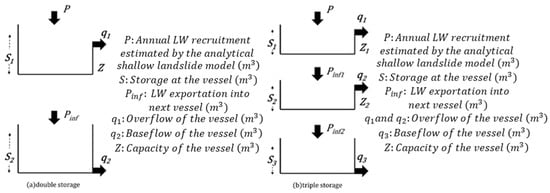
Figure 7.
A conceptual scheme of the double storage function model (a) and the triple storage function model (b) (modified from Komori et al., 2021) [43].
2.3.1. Triple Storage Function Model
For equations related to the double storage tank model case, refer to Komori et al. (2021) [43]. The details of the triple storage function model are described below.
The first vessel utilized in this study comprises three components. One part simulates the direct export of LW as overflow from the first vessel (), while another part simulates LW storage at the stream channel as storage at the first vessel () and its subsequent exportation into the second vessel (). In the modelling framework, is recharged by annual LW recruitment () and occurs once the capacity of the first vessel () is exceeded. The first vessel can be represented as follows:
where is parameter and is time (in years).
The second vessel used in this study consists of three parts. One part simulates the direct export of LW as overflow from the first vessel () and the other part simulates LW storage at the stream channel as storage at the first vessel () and its exportation into the second vessel (). In the modelling framework, S2 is recharged by annual LW recruitment () and q2 occurs once the capacity of the first vessel () is exceeded. The first vessel can be written as follows:
The third vessel used in this study consists of two parts. One part simulates past LW storage at the stream channel, represented as storage in the second vessel (), while the other part simulates the continuous LW export from the second vessel as the base flow (). Within the modelling framework, is recharged by and is nonlinearly influenced by an increase in . The secondary vessel can be represented using a nonlinear storage function model, as outlined below:
where and are parameters.
For the initial condition of the storage of LW in the model, Komori et al. (2021) [43] examined the spin-up of using the value of obtained from the model run inputting a series of annual LW recruitment during the target period from zero to three times repeatedly. As a result, the reproductivity of the model was the best in the case of a spin-up of zero times and, therefore, we applied this spin-up for the double storage function model. On the other hand, we tentatively set and for the triple storage function model as 30%, because of elevated computational costs for spin-up.
2.3.2. Optimisation of Parameters and Evaluation of Reproducibility of the Volume of LW Export
Parameters in the model are determined by the iterative approximation of the model with all combinations of parameters (Table 2 and Table 3), with the combination that maximises the following Nash–Sutcliffe efficiency () [47] between the total amount of simulated LW exports ( = + or = + + ) and :
where is the analysis period (in years), is a year, and is the period average of (in ). is used as an index to evaluate the suitability of a flow hydrograph considering the magnitude of flow rate variability. Furthermore, indicated the closer the value is to 1, the better the accuracy of the model and indicated a value higher than 0.4 for satisfactory results, with reproducibility of the simulation.

Table 2.
Initial, end, and incremental values of parameters in the double storage function model.

Table 3.
Initial, end, and incremental values of parameters in the triple storage function model.
Figure 8 shows the for a combination of parameters and when the parameters and were 0.0151 and 0.51, respectively, as an example of a parameter recognised at a dam reservoir watershed. Here, the names of the dams cannot be revealed because of the restrictions on data use. The red circle was the parameter combinations for which the is highest in this condition. The recognition of these parameters was successively calculated according to Table 2 for the double storage function model, or Table 3 for the triple storage function model, and the parameter combination with the highest was adopted as the recognised parameter.
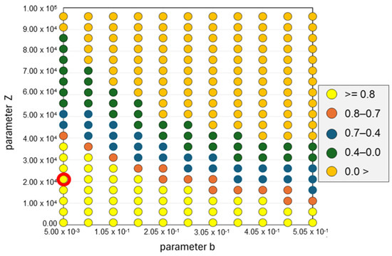
Figure 8.
for a combination of parameters and when the parameters and were 0.0151 and 0.51, respectively, as an example of parameter recognition at a dam reservoir watershed. The red circle was the parameter combinations for which the was the highest in this condition.
This parameter recognition was implemented at each of the 212 dam reservoir watersheds in both the double and triple storage function models, aiming to determine the most suitable model that corresponds to the distinct characteristics of the watershed.
2.4. Frequency Analysis
To verify the characteristics of LW export examined by double and triple storage function models, frequency analysis was performed to compare the cumulative values of the estimated annual volume for LW recruitment across dam reservoir watersheds over periods ranging from 1 to 6 years with the annual volume of LW export. The outcomes were summarized by the determination of the count of cumulative years exhibiting correlation coefficients surpassing the threshold of 0.3 (see Section 3). Spearman’s rank correlation analysis was utilized to compute the correlation coefficients, while p-values were derived using the Wilcoxon signed-rank test. These statistical analyses were executed through Python 3.10.9, employing the “spearman” function from the SciPy library.
3. Results and Discussions
The model was applied to 212 dam reservoir watersheds across Japan and the results of the model application are presented in Table 4 and Table 5. Table 4 shows the number of watersheds in each region where the volume of LW export was successfully reproduced ( > 0.4) using the double or triple storage function models (hereinafter, referred to as Group 1 and Group 2). Table 5 shows the number of watersheds in each region where the volume of LW export was successfully reproduced ( > 0.4) by both of them (hereinafter, referred to as Group 3) and the number of watersheds where the higher was obtained using either of them (hereinafter, referred to as Group 4). In Table 4, the number of dam reservoir watersheds for which reproducibility was obtained for Group 1 was 30, indicating that the LW export characteristics could be explained by two export characteristics, as follows: direct export and baseflow, as described by Komori et al. (2021) [43]. On the other hand, in the Chubu, Kinki, and Shikoku regions, all of the dam reservoir watersheds could not be reproduced in terms of LW export volume. It was estimated that the LW export in the dam reservoir watersheds in these regions cannot be explained by the two export characteristics.

Table 4.
The number of watersheds in each region where the volume of LW export was successfully reproduced ( > 0.4) using the double (Group 1) or triple (Group 2) storage function models.

Table 5.
The number of watersheds in each region where the volume of LW export was successfully reproduced ( > 0.4) by both of the double and triple storage function models (Group 3), and the number of watersheds where the higher was obtained using either of them (Group 4).
The number of dam reservoir watersheds for which reproducibility was obtained for Group 2 was 116. More than 50% of all target dam reservoir watersheds across Japan, with the exception of the Kanto region, were able to reproduce LW export volumes using the triple storage function model, suggesting that many watersheds across Japan have three LW export characteristics.
In Table 5, the number of dam reservoir watersheds for which reproducibility was obtained for the best choice was 134, which means that reproducibility was obtained in the LW-Budget model in more than 50% of the target dam reservoir watersheds. This confirmed the hypotheses regarding the relationship between LW recruitment and landslides triggered by intense rainfalls, as well as the connection between LW export and the long-term LW budget on an annual scale in Japan [43]. In each region, reproducibility of LW export volumes was obtained in 75.0% of the target dam reservoir watersheds in the Tohoku and Hokuriku regions, the highest proportion. In all regions, the LW export volume was reproduced in more than 50.0% of the target dam reservoir watersheds, confirming the generality of the LW-Budget across Japan.
As cases of satisfactory and unsatisfactory results are present in each of Groups 1, 2, and 3, Figure 9, Figure 10 and Figure 11 show plots of , , and , which were simulated using the LW-Budget model, using the double (Figure 9a, Figure 10a and Figure 11a) and triple (Figure 9b, Figure 10b and Figure 11b) storage function models at dam reservoir watersheds. Here, the names of the dams cannot be revealed because of the restrictions of data use, so we used pseudonyms instead of the actual dam names. In Figure 9, the maximum was recorded in 2005 at the A dam, when the maximum was recorded. On the other hand, was almost constant after 2005, although a larger was recorded in 2014, 2016, 2018, and 2020, every 2 years. The increase in could be reproduced in 2005 by the double storage function model (Figure 9a). On the other hand, the constant after 2005 could not be reproduced by the triple storage function model (Figure 9b). Therefore, it was considered that the LW export characteristics at the A dam could be explained by the following two export characteristics: direct export and baseflow, as described by Komori et al. (2021) [43].
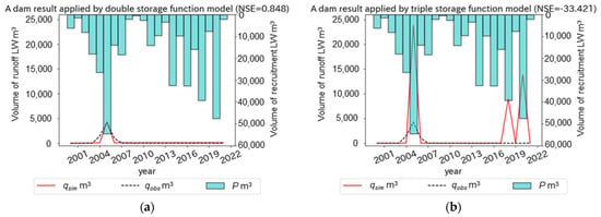
Figure 9.
Plots of , , , and the for annual LW export simulation using the double (a) and triple (b) storage function models at a dam reservoir watershed as a case of satisfactory and unsatisfactory results in Group 1.
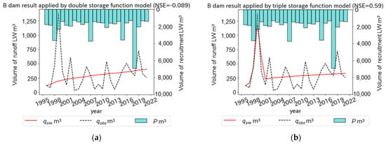
Figure 10.
Plots of , , , and the for annual LW export simulation using the double (a) and triple (b) storage function models at a dam reservoir watershed as a case of satisfactory and unsatisfactory results in Group 2.
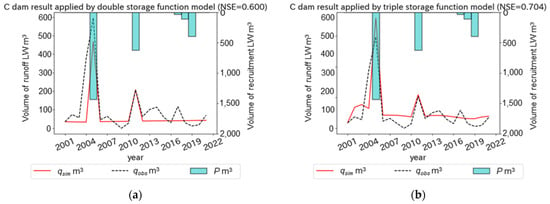
Figure 11.
Plots of , , , and the for annual LW export simulation using the double (a) and triple (b) storage function models at a dam reservoir watershed as a case of satisfactory results in Group 3.
In Figure 10, the maximum was recorded in 1999 at the B dam, although was recorded in 1998, 2007, 2015, and 2018, larger than in 1999. The increase in could be reproduced in 1999 by the triple storage function model (Figure 10b), but not the double storage function model (Figure 10a). This would suggest that the LW export characteristics at the B dam could be explained by the following three export characteristics: direct export, baseflow, and one other export. In addition, the reproduction of the increase in in 1999 by for three years showed the significance of the setting of the initial condition of the storage of LW in the model.
In Figure 11, the maximum was recorded in 2005 at the C dam, although was recorded only 5 years in 2005, 2011, 2017, 2018, and 2019. The increase in could be reproduced in 2005 by both the double and triple storage function models (Figure 11a,b). This would suggest that the LW export characteristics at the C dam could be explained by either two or three export characteristics. Furthermore, the reproduction of the increase in in 2005 by only in 2005 also showed the significance of the setting of the initial condition of the storage of LW in the model, in the same manner as in Figure 10.
As cases of unsatisfactory results are present for both double and triple storage function models, Figure 12 and Figure 13 show plots of , , and , which were simulated using the LW-Budget model, using the double (Figure 12a and Figure 13a) and triple (Figure 12b and Figure 13b) storage function models at dam reservoir watersheds. Here, the names of the dams cannot be revealed because of the restrictions of data use, so we used pseudonyms instead of the actual dam names. In Figure 12, although the maximum was recorded in 2007 and 2012 at the D dam, the increase in could not be reproduced in 2007 and 2012 by both the double and triple storage function models (Figure 12a,b). Therefore, it was considered that the LW export characteristics at the D dam could not be explained by two or three export characteristics.
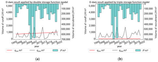
Figure 12.
Plots of , , , and the for annual LW export simulation using the double (a) and triple (b) storage function models at a dam reservoir watershed as a case of unsatisfactory results.
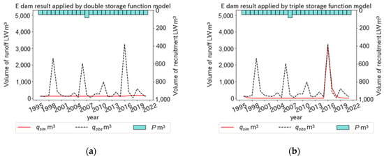
Figure 13.
Plots of , , , and the for annual LW export simulation using the double (a) and triple (b) storage function models at a dam reservoir watershed as a case of unsatisfactory results.
In Figure 13, the larger were recorded in 1999, 2005, and 2016 at the E dam, although was remarkably smaller than other dams and was almost constant. The increase in could not be reproduced in the larger by both the double and triple storage function models (Figure 13a,b). Therefore, it was considered that the LW export characteristics at the E dam could not be explained by LW recruitment with landslides triggered by intense rainfalls, as described by Komori et al. (2021) [43].
To examine the statistical differences in the variables in the watershed where LW characteristics were reproduced on the application of the double and triple storage function models, the Mann–Whitney U test was performed. Note that this is one of the non-parametric statistical tests and is based on the null hypothesis that two populations are the same, if a particular population tends to have a larger value than the other. The results are shown in Table 6. Here, the significance level was set at 5% and the watershed variables were selected based on Seo et al. (2009) [48], analysing LW characteristics for dam reservoir watersheds across Japan. The watershed variable that satisfied the 5% significance level was only the watershed area. Namely, a statistical difference in the watershed area was recognised between the double and triple storage function models. This indicated that the double storage function model tended to fit larger watershed areas, while the triple storage function model tended to fit smaller watershed areas. In addition, no statistical differences were shown for the other watershed variables other than the watershed area, making it difficult to explain the differences in LW export characteristics between the double and triple storage function models.

Table 6.
Results of the Mann–Whitney U-tests of variables in watersheds where LW characteristics were reproduced on the application of the double and triple storage function models.
In Seo et al. (2009), watershed area and latitude were employed as explanatory variables in the statistical analysis of LW exports observed in dam reservoir watersheds across Japan [48]. This was confirmed by the authors’ previous studies and it was inferred that latitude was employed as a parameter that could explain differences in precipitation characteristics across Japan [49]. In this study, it is assumed that only the watershed area was adopted, because differences in precipitation characteristics across Japan have already been taken into account in LW-Budget, where precipitation was used as an input value.
Table 7 shows the number and proportion of cumulative years that recorded correlation coefficients above the threshold of 0.3, through correlation analysis between six patterns of cumulative accumulated recruitment LW and runoff LW. In the all-target watersheds, 101 watersheds out of 212 watersheds have over 0.3 correlation coefficients. In the watersheds successfully reproduced using the triple storage function model, the results of six patterns are 16, 8, 13, 4, 3, and 6 watersheds, respectively. These values differ significantly in number compared to the watersheds for which reproducibility was obtained in the double storage function model, for values of three or more patterns to be gained. Finally, the double storage function model was 59% of the total for the sum of one and two (10 watersheds) and the three storage function model was 74% of the total for the sum of one, two, and three (37 watersheds). This would suggest that the double storage function model is more likely to be applied to cases with 1–2 runoff characteristics and the triple storage function model to cases with 1–3 runoff characteristics.

Table 7.
The number and proportion of cumulative years that recorded correlation coefficients above the threshold of 0.3, through correlation analysis between six patterns of cumulative accumulated recruitment LW and runoff LW.
4. Conclusions
In this study, we aimed to verify the hypotheses proposed by the authors on the relationship between LW recruitment and landslides triggered by intense rainfalls, as well as LW export and the long-term LW budget on an annual scale [43], applying LW-Budget to 212 dam reservoir watersheds across Japan. We used LW-Budget with not only double but also triple storage function with the lumped hydrological method at a watershed scale for the LW entrainment to examine the hypotheses. The objective is to produce new, testable hypotheses on the characteristics of LW export and the long-term LW budget, on an annual scale.
Application of the model to target watersheds across the country resulted in reproducibility in the estimation of runoff volume in 134 of the targeted dam reservoir watersheds, which were 63.2% of the target basins. This indicated that our results verified these two relationships as primary relationships and slope failure, which is caused by large wood recruitment, and long-term budget of large wood are responsible for large wood exports on an annual scale.
On the other hand, in 36.8% of the target dam reservoir watersheds, LW-Budget could not reproduce the volume of LW export. In LW recruitment, factors other than slope failure, such as LW recruitment from riparian forests by floods, have been reported in Japan. In addition, the authors have already found, in previous studies, that the estimation of the amount of LW recruitment could not be attributed to the annual maximum 24 h precipitation in one case. It will, therefore, be important to develop new approaches for estimating LW recruitment from sources other than slope failure and to upgrade LW-Budget from annual to shorter time scales. In LW entrainment, the estimated LW export volume could only be explained by the watershed area. This suggests that the micro-scale LW dynamics were not well captured by LW-Budget at the dam reservoir watershed scale. Therefore, it will be important to upgrade the LW-Budget for applications at smaller catchment scales. It is also important to understand the differences between the double and triple storage function models, to better understand the differences in runoff systems and other aspects of LW export.
Finally, for effective LW management that balances natural hazard mitigation and ecosystem conservation in the era of global warming, it is essential to understand the characteristics of LW export at the watershed scale. To this end, it is essential to advance the understanding of a series of dynamics of LW export and to quantitatively elucidate the combined effects of biological, physical, and anthropogenic factors. In this respect, it was a very significant achievement that the generality of LW export characteristics based on a series of dynamics of LW export in Japan was demonstrated in this study. Furthermore, the LW-Budget is a model that can estimate the potential LW export volume including the volume of stored LW in the watershed using only precipitation as input data. We are convinced that LW-Budget can help to design the LW management on river and dam reservoirs, as it can predict potential LW export volumes by using predicted precipitation in the future or probable precipitation.
Author Contributions
Conceptualization, D.K.; methodology, D.K. and Y.A.; formal analysis and investigation, D.K., Y.A. and S.P.; writing—original draft preparation, D.K. and Y.A.; writing—review and editing, D.K. and S.P.; supervision, D.K.; funding acquisition, D.K. All authors have read and agreed to the published version of the manuscript.
Funding
This research was partly supported by the Ministry of Land, Infrastructure, Transport and Tourism (MLIT), according to the ‘Improving the reproducibility of large wood dynamics analysis using the integrated large wood export model (PI: Daisuke Komori)’ and the Grants in Aid for Fostering Joint International Research (19KK0362, PI: Daisuke Komori) from Japan Society for the Promotion of Science, Japan.
Data Availability Statement
The are not shared due to the data policy of the MILT. Radar-AMeDAS rainfall of the JMA are available from the public data source; https://www.data.jma.go.jp/gmd/risk/obsdl/index.php, accessed on 20 November 2023 (in Japanese). Other data sets analysed during the current study are available from the corresponding author on reasonable request.
Acknowledgments
The authors would like to thank the Water Resources Environment Technology Centre and the Japanese Ministry of Land, Infrastructure and Transport (MLIT) for their assistance in providing and collecting data on LW. The authors also thank Seiki Kawagoe, Katsuhiro Nakao, and So Kazama for their valuable advice. This research was funded by the Ministry of Land, Infrastructure, Transport and Tourism (MLIT), according to the ‘Improving the reproducibility of large wood dynamics analysis using the integrated large wood export model (PI: Daisuke Komori)’ and the Grants in Aid for Fostering Joint International Research (19KK0362, PI: Daisuke Komori) from the Ministry of Education, Science and Culture, Japan.
Conflicts of Interest
The authors declare no conflicts of interest.
References
- Ruiz-Villanueva, V.; Piégay, H.; Gurnell, A.M.; Marston, R.A.; Stoffel, M. Recent advances qualifying the large wood dynamics in river basins, new method and remaining challenges. Rev. Geophys. 2016, 54, 611–652. [Google Scholar] [CrossRef]
- Montgomery, D.R.; Collins, B.D.; Buffington, J.M.; Abbe, T.B. Geomorphic effects of wood in rivers. Am. Fish. Soc. Symp. 2003, 37, 21–47. [Google Scholar]
- Wohl, E.; Scott, D.N. Wood and sediment storage and dynamics in river corridors. Earth Surf. Process. Landf. 2017, 42, 5–23. [Google Scholar] [CrossRef]
- Prescott, C.E.; Laiho, R. The Nutritional Significant of Coarse Woody Debris in Three Rocky Mountain Coniferous Forests; USDA Forest Service General Technical Report PSW-GTR-181; USDA Forest Service: Washington, DC, USA, 2002; pp. 381–392.
- Yan, E.; Wang, X.; Huang, J. Concept and classification of coarse woody debris in forest ecosystems. Front. Biol. China 2006, 1, 76–84. [Google Scholar] [CrossRef]
- Sakai, Y.; Ugawa, S.; Ishizuka, S.; Takahashi, M.; Takenaka, C. Wood density and carbon and nitrogen concentrations in deadwood of Chamaecyparis obtuse and Crytomeria japonica. Soil Sci. Plant Nutri. 2012, 58, 526–537. [Google Scholar] [CrossRef]
- Chao, K.J.; Chen, Y.S.; Song, G.Z.M.; Chang, Y.M.; Sheue, C.R.; Phillips, O.L.; Hsieh, C.F. Carbon concentration declines with decay class in tropical forest woody debris. For. Ecol. Manag. 2012, 391, 75–85. [Google Scholar] [CrossRef]
- Fukasawa, Y.; Katsumata, S.; Mori, A.S.; Osono, T.; Takeda, H. Accumulation and decay dynamics of coarse woody debris in a Japanese old-growth subalpine coniferous forest. Ecol. Res. 2014, 29, 257–269. [Google Scholar] [CrossRef]
- Jomura, M.; Kominami, Y.; Tamai, K.; Miyama, T.; Goto, Y.; Dannoura, M.; Kanazawa, Y. The carbon budget of coarse woody debris in a temperate broad-leaved secondary forest in Japan. Tellus 2007, 59, 211–222. [Google Scholar] [CrossRef]
- Kim, R.H.; Son, Y.; Lim, J.H.; Lee, I.K.; Seo, K.W.; Koo, J.W.; Noh, N.J.; Ryu, S.-R.; Hong, S.K.; Ihm, B.S. Coarse woody debris mass and nutrients in forest ecosystems of Korea. Ecol. Res. 2006, 21, 819–827. [Google Scholar] [CrossRef]
- Woods, K.D. Multi-decade biomass dynamics in an oil-growth hemlock-northern hardwood forest, Michigan, USA. PeerJ 2014, 2, e598. [Google Scholar] [CrossRef]
- Mao, L.; Andreoli, A.; Iroumé, A.; Comiti, F.; Lenzi, M.A. Dynamics and management alternatives of in-channel large wood in mountain basins of the southern Andes. Bosque 2013, 34, 15–16. [Google Scholar] [CrossRef]
- Chaithong, T.; Komori, D.; Sukegawa, Y.; Anzai, S. Estimating woody debris recruitment in a stream caused by a typhoon-induced landslide: A case study of Typhoon Lionrock in Iwaizumi, Iwate prefecture, Japan. Geomat. Nat. Hazards Risk 2018, 9, 1071–1084. [Google Scholar] [CrossRef]
- Lucía, F.; Comiti, M.; Borga, M.; Cavalli, M. Large wood recruitment and transport during a severe flash flood in north-western Italy. Eng. Geol. Soc. Territ. 2014, 3, 159–162. [Google Scholar]
- Komori, D.; Hendrawan, V.S.A.; Ichiba, A.; Yamada, K.; Goda, A. Mechanism of rainfall inundation caused by the 2019 Typhoon Hagibis in Iwate prefecture coastal zone, Japan. J. JSCE 2022, 10, 195–205. [Google Scholar] [CrossRef] [PubMed]
- Gippel, C.J.; Finlayson, B.L.; O’Neill, I.C. Distribution and hydraulic significance of large woody debris in a lowland Australian river. Hydrobiologia 1996, 318, 179–194. [Google Scholar] [CrossRef]
- Beebe, J.T. Flume studies of the effect of perpendicular log obstructions on flow patterns and bed topography. Great Lakes Geogr. 2000, 7, 9–25. [Google Scholar]
- Yamada, T.; Yasuhiro, D.; Noriyuki, M.; Takaaki, A. Woody debris trapping by impermeable type Sabo dam. J. Jpn. Soc. Eros. Control Eng. 1999, 52, 18–23. (In Japanese) [Google Scholar]
- Benda, L.; Miller, D.; Marin, D.; Bilby, R.; Veldhuisen, C.; Dunne, T. Wood recruitment process and wood budgeting. Am. Fish. Soc. Symp. 2003, 37, 49–73. [Google Scholar]
- Chen, S.C.; Chao, Y.C.; Chan, H.C. Typhoon-dominated influence on wood debris distribution and transportation in a high gradient headwater catchment. J. Mt. Sci. 2013, 10, 509–521. [Google Scholar] [CrossRef]
- Steeb, N.; Rickenmann, D.; Badoux, A.; Rickli, C.; Waldner, P. Large wood recruitment processes and transported volumes in Swiss mountain streams during the extreme flood of August 2005. Geomorphology 2017, 279, 112–127. [Google Scholar] [CrossRef]
- Rickli, C.; Badoux, A.; Rickenmann, D.; Steeb, A.; Waldner, P. Large wood potential, piece characteristics, and flood effects in Swiss mountain streams. Phys. Geogr. 2018, 39, 542–564. [Google Scholar] [CrossRef]
- Murakami, Y.; Shimizu, O.; Sato, H.; Yamada, T. Sediment-related disaster caused by Typhoon 0310 (Etau) in Hidaka Region of Hokkaido, Japan. J. Jpn. Soc. Eros. Control Eng. 2008, 1, 30–37. [Google Scholar] [CrossRef][Green Version]
- Montgomery, D.R.; Buffington, J.M. Channel Classification, Prediction of Channel Response, and Assessment of Channel Condition; Report TFW-Si-110-93-002; the SHAMW Committee of the Washington State Timber/Fish/Wildlife Agreement. 1993. Available online: https://geo.nwifc.org/CMER/PublicDocs/TFWDocs/TFW_SH10_93_002%20Channel%20Classification%20Prediction%20of%20Channel%20Response%20and%20Assessment%20of%20Channe.pdf (accessed on 20 November 2023).
- Ruiz-Villanueva, V.; Diez-Herrero, A.; Ballesteros, J.A.; Bodoque, J.M. Potential large woody debris recruitment due to landslides, bank erosion and floods in mountain basins: A quantitative estimation approach. River Res. Appl. 2014, 30, 81–97. [Google Scholar] [CrossRef]
- Sickle, J.V.; Gregory, S.V. Modeling inputs of large woody debris to streams from falling trees. Can. J. For. Res. 1990, 20, 1593–1601. [Google Scholar] [CrossRef]
- Mazzorana, B.; Zischg, A.; Largiader, A.; Hubl, J. Hazard index maps for woody material recruitment and transport in alpine catchments. Nat. Hazards Earth Syst. Sci. 2009, 9, 197–209. [Google Scholar] [CrossRef]
- Scheip, C.M.; Wegmann, K.W. HazMapper: A global open-source natural hazard mapping application in Google Earth Engine. Nat. Hazards Earth Syst. Sci. 2021, 21, 1495–1511. [Google Scholar] [CrossRef]
- Phakdimek, S.; Komori, D.; Chaithong, T. Combination of optical images and SAR images for detecting landslide scars, using a classification and regression tree. Int. J. Remote Sens. 2023, 44, 3572–3606. [Google Scholar] [CrossRef]
- Seo, J.; Nakamura, F.; Chun, K.W.; Kim, S.W.; Grant, G.E. Precipitation patterns control the distribution and export of large wood at the catchment scale. Hydrol. Process. 2015, 29, 5044–5057. [Google Scholar] [CrossRef]
- Seo, J.; Nakamura, F. Scale-dependent controls upon the fluvial export of large wood from river catchments. Earth Surf. Process. Landf. 2009, 34, 786–800. [Google Scholar] [CrossRef]
- Chaithong, T.; Komori, D.; Sukegawa, Y.; Touge, Y.; Mitobe, Y.; Anzai, S. Landslides and precipitation characteristics during the typhoon Lionrock in Iwate prefecture, Japan. Int. J. GEOMATE 2018, 14, 109–114. [Google Scholar] [CrossRef]
- Crowther, T.W.; Glick, H.B.; Covey, K.R.; Bettigole, C.; Maynard, D.S.; Thomas, S.M.; Smith, J.R.; Hintler, G.; Duguid, M.C.; Amatulli, G.; et al. Mapping tree density at a global scale. Nature 2015, 525, 201–205. [Google Scholar] [CrossRef]
- Chaithong, T.; Komori, D. Hydrological-geotechnical model to assess the extreme rainfall-induced shallow landslides. J. Jpn. Soc. Civ. Eng. 2017, 73, 223–228. [Google Scholar] [CrossRef]
- Martin, D.J.; Benda, L.E. Patterns of instream wood recruitment and transport at the watershed scale. Trans. Am. Fish. Soc. 2001, 130, 940–958. [Google Scholar] [CrossRef]
- Collins, B.D.; Montgomery, D.R.; Fetherston, K.L.; Abbe, T.B. The floodplain large-wood cycle hypothesis: A mechanism for the physical and biotic structuring of temperate forested alluvial valleys in the North Pacific coastal ecoregion. Geomorphology 2012, 139–140, 460–470. [Google Scholar] [CrossRef]
- Boivin, M.; Buffin-Bélanger, T.; Piégay, H. Estimation of large wood budgets in a watershed and river corridor at interdecadal to interannual scales in a cold-temperate fluvial system. Earth Surf. Process. Landf. 2017, 42, 2199–2213. [Google Scholar] [CrossRef]
- Mozzorana, B.; Hübl, J.; Zischg, A.; Largiader, A. Modelling woody material transport and deposition in alpine rivers. Nat. Hazards 2011, 56, 425–449. [Google Scholar] [CrossRef]
- Zischg, A.; Galatioto, N.; Deplazes, S.; Weingarter, R.; Mazzorana, B. Modelling spatiotemporal dynamics of large wood recruitment, transport, and deposition at the river research scale during extreme floods. Water 2018, 10, 1134. [Google Scholar] [CrossRef]
- Benda, L.E.; Sias, J.C. A quantitative framework for evaluating the mass balance of in-stream organic debris. For. Ecol. Manag. 2003, 172, 1–16. [Google Scholar] [CrossRef]
- Hassan, M.A.; Bird, S.; Reid, D.; Hogan, D. Simulated wood budgets in two mountain streams. Geomorphology 2016, 259, 119–133. [Google Scholar] [CrossRef]
- Pettit, N.E.; Naiman, R.J.; Rogers, K.H.; Little, J.E. Post–flooding distribution and characteristics of large woody debris piles along the semi-arid Sabie River South Africa. River Res. Appl. 2005, 21, 27–38. [Google Scholar] [CrossRef]
- Komori, D.; Sukegawa, Y.; Chaithong, T.; Kazama, S. Modelling of large wood export at a watershed scale. Earth Surf. Process. Landf. 2022, 47, 688–696. [Google Scholar] [CrossRef]
- Phakdimek, S.; Nakamura, M.; Abe, Y.; Komori, D. The Sensitivity of spatial variation soil thickness and rainfall on shallow landslide triggering patterns. J. Jpn. Soc. Civ. Eng. 2022, 78, 117–124. [Google Scholar] [CrossRef] [PubMed]
- Rosso, R.; Rulli, M.C.; Vannucchi, G. A physically based model for the hydraulic control on shallow landsliding. Water Resour. Res. 2006, 42, 1–16. [Google Scholar] [CrossRef]
- Young, R.; Farrar, J.; Howard, A. Earth Manual Part 1, 3rd ed.; US Government Printing Office: Washington, DC, USA; U.S. Department of the Interior Bureau of Reclamation: Washington, DC, USA, 1998.
- Nash, J.E.; Sutcliffe, J.V. River flow forecasting through conceptual models part I—A discussion of principles. J. Hydrol. 1970, 10, 282–290. [Google Scholar] [CrossRef]
- Seo, J.; Nakamura, F.; Nakano, D.; Ichiyanagi, H.; Chun, K.W. Factors controlling the fluvial export of large woody debris, and its contribution to organic carbon budgets at watershed scales. Water Resour. Res. 2008, 44, W04428. [Google Scholar] [CrossRef]
- Sukegawa, Y.; Komori, D. Statistical analysis of woody debris volume to specify mechanism of recruitment in dam reservoirs in Japan. J. Jpn. Soc. Civ. Eng. 2017, 73, 55–61. (In Japanese) [Google Scholar]
Disclaimer/Publisher’s Note: The statements, opinions and data contained in all publications are solely those of the individual author(s) and contributor(s) and not of MDPI and/or the editor(s). MDPI and/or the editor(s) disclaim responsibility for any injury to people or property resulting from any ideas, methods, instructions or products referred to in the content. |
© 2024 by the authors. Licensee MDPI, Basel, Switzerland. This article is an open access article distributed under the terms and conditions of the Creative Commons Attribution (CC BY) license (https://creativecommons.org/licenses/by/4.0/).