Approximate Solutions for Horizontal Unconfined Aquifers in the Buildup Phase

Abstract

We construct approximate analytical solutions of the Boussinesq equation for horizontal unconfined aquifers in the buildup phase under constant recharge and zero-inflow conditions. We employ a variety of methods, which include wave solutions, self-similar solutions, and two classical linear approximations of the Boussinesq equation (linear and quadratic), to explore the behavior and performance of the solutions derived from each method against the Boussinesq equation and the exact (non-closed form) analytical solutions. We find that the wave approximation, which is of a conceptual nature, encapsulates quite faithfully the characteristics of the nonlinear Boussinesq equation solution and, overall, performs much better than the other methods, for which the relatively low performance can be attributed to the specific mathematical features of their construction. These endeavors might be useful for theoretical and modeling purposes related to this problem.

1. Introduction

The study of groundwater dynamics is important in hydraulic engineering because it focuses on the description of the fluid flow through aquifers, either horizontal or sloped. The groundwater flow through aquifers is well described by the Boussinesq equation [1,2]. This equation can be derived utilizing the concepts of the classical Dupuit assumptions, which consider a 2D horizontally infinite homogeneous aquifer under fully saturated conditions, providing the basis for a simplified framework for analyzing groundwater flow under idealized conditions and enabling the derivation of analytical solutions. This assumption was later improved by Forchheimer [3,4,5]. Owing to the dynamic nature of the Boussinesq equation in various groundwater flow applications, it is not surprising that significant theoretical and experimental work has been devoted to searching for its exact and approximate solutions when tailored for specific applications after constructing the mathematical problem with appropriate boundary conditions, leading to numerous studies of its accuracy. The main reason for the difficulty in obtaining solutions is because this fundamental equation is nonlinear. The nonlinearity arises from dimensional considerations and the assumption that the vertical flow can be considered as being homogeneous, which makes the flux of fluids proportional to the free-surface height times the hydraulic gradient. Therefore, solutions of the Boussinesq equation are important, and the topic of reaching either analytical or approximate solutions remains an active research topic. The current set of known solutions is by no means exhaustive, and many analytical solutions are being continuously proposed by considering different initial and boundary conditions representative for the problem under investigation [6,7,8,9,10,11,12,13,14,15,16,17,18,19,20,21,22].

Analytical solutions are routinely used not only for benchmarking and checking the numerical code’s accuracy (especially in nonlinear problems) but also for giving important insights into the physical problem to be used conceptually for building more complex and realistically relevant problems. In the problem at hand, we start off with an empty aquifer, which fills under constant recharge. This causes a sudden change in the water level (early buildup phase) of a horizontal unconfined aquifer. This presents a basic problem that draws attention as a benchmark. During the early times, or the buildup phase, there are very few exact solutions. For the special problem of groundwater flowing in a semi-infinite domain and for the zero-recharge rate, existing solutions consider quadratic polynomials for describing the flow from the inlet and up to a certain distance in horizontal [11] and inclined [23] aquifers. These solutions are derived using a similarity transformation, which proves to be quite cumbersome [24]. As an alternative method, self-similar solutions have been proposed [25], which draw particular interest for the latest problem of CO₂ sequestration [26]. Another more attractive method is the use of power series solutions for the self-similar form of the Boussinesq equation for the problem of horizontal aquifers, considering a power law boundary condition for the water depth at inlets. The latter form of the solution was obtained in [8,10,11,15,18,21,27,28,29,30,31,32]. These solutions are useful for the computation of flow volumes either injected into or pumped out from aquifers. For the case of groundwater flowing in a horizontal finite aquifer at a zero-recharge rate, the solution of the equation can be obtained by assuming the separation of variables [2,7]. This is actually an exact asymptotic solution of the horizontal aquifer recession phase for late times. A rather interesting method of solution is the kinematic wave, by which the nonlinear term in the Boussinesq equation can be dropped. Although it is an approximate solution, it can also be used for aquifers having steep slopes, high conductivities, or low recharge rates, cases that fall within the low values of the Henderson and Wooding parameter. The benefit is that the solution becomes less and less approximate for lower values of this parameter, eventually reaching, asymptotically, the exact form of the solution [1,33,34,35,36,37,38,39].

Some problems involving the fundamental Boussinesq equation do not have an exact solution, and another family of methods is applied to investigate the fundamental equations by means of approximate analytical solutions. The approximate solutions are obtained using different mathematical techniques in which, usually, the final expressions are in the form of series expansions of functions constructed for each case that is examined. These include polynomial series expansions, implicit forms, explicit closed-forms, and, lately, fuzzy solutions requiring iterative procedures to converge [7,16,17,21,30,31,32,40,41,42,43]. The approximate solutions, if they can be developed, present the advantages that, in most cases, are simple and that the mathematical manipulations can be fairly accommodated because they are straightforward and can be easily implemented. This is exactly the motivation behind this work. It should be mentioned that none of these studies, with the exception of [39], focuses on the problem that is a subject of the present work, that is, the early time behavior of horizontal aquifers during the buildup phase.

In this work, we investigate novel approximate solutions for subsurface flows over a horizontal bed during the early buildup phase of unconfined aquifers under constant discharge and hydraulic conditions. We employ certain naturally applicable approximations in this problem, aiming to explore their behavior and performance in reproducing the characteristics of the nonlinear Boussinesq equation solutions. This paper is organized as follows: in Section 2, we present the derivation of the Boussinesq equation for a steady-state fluid flow. In Section 3, we present the novel approximate solutions during the early buildup phase by formulating the Boussinesq equation in its dimensionless form and applying the methods of the wave approximation, self-similar solutions, and linearizations (linear and quadratic). Finally, in Section 4, the major outcomes from this work are emphasized.

2. Steady-State Fluid Flow in Horizontal Unconfined Aquifers

The formulation that will be presented in this section has the usual assumptions of aquifer modeling susceptible to an analytical treatment, which are summarized as follows: The aquifer is assumed to be horizontal (1) with a flat bed; (2) with uniform, in space and time, hydraulic properties; (3) with a uniform recharge rate; and (4) with simple boundary conditions. Certain types of reservoirs to which we can apply the results of this work include the alluvial aquifers, which are mostly composed of unconsolidated sediments hosting various sizes of grains, like gravel, sand, silt, and clay, that are deposited by rivers and streams. These aquifers often have relatively homogeneous properties and can exhibit flat horizontal beds over large areas, making them amenable to 1D approximations. Another type of reservoir is one that is formed in deltaic environments where sediments are deposited in deltas, which can have relatively flat horizontal beds, especially in the areas further away from the deltaic front. Finally, coastal aquifers are also another candidate of sedimentary deposits laid down under uniform depositional conditions satisfying the assumptions behind the application of the Boussinesq equation.

This section intends to recapitulate certain known results to make our presentation self-contained. We shall assume a uniform and constant hydraulic conductivity (k) and porosity (n) throughout the aquifer. The recharge rate (r) will also be assumed to be constant, and the resulting flow will be considered as being saturated and, effectively, one-dimensional. The impermeable bottom of the aquifer is assumed to be flat and horizontal. A sketch of the aquifer is given in Figure 1.

By the Dupuit–Forchheimer approximation, the flow per unit of width for each time instant (t) and for each position (x) is given as follows [5,44,45]:

$$q = - kh\frac{\partial h}{\partial x}$$

(1)

where h is the water table’s depth at position x and at time t. The continuity equation (equation of mass conservation) expresses that the total amount of water flowing in any part of the aquifer locally, r, is equal to the sum of the amount of water flowing through it, $\partial q/\partial x$, plus the change in the storage capacity, $n\partial h/\partial t$, which in this case is written as follows:

$$n\frac{\partial h}{\partial t} + \frac{\partial q}{\partial x} = r$$

(2)

Combining Equations (1) and (2), we obtain the Boussinesq equation for the horizontal aquifer as follows:

$$n\frac{\partial h}{\partial t}-k\frac{\partial }{\partial x}\left[h\frac{\partial h}{\partial x}\right]=r$$

(3)

The boundary conditions that we will impose are as follows:

$$\frac{\partial h}{\partial x}(0,t)=0$$

(4)

$$h(L,t)=0$$

(5)

which express that there is no inflow at the point x = 0 and that the water table has a zero depth at the outlet of the aquifer. Also, as we are interested in the filling phase of the aquifer, we will impose the following initial condition:

$$h(x,0)=0$$

(6)

In the long run, the system will be led to a balance between recharging and discharging, i.e., the steady state where there is no time change. The steady-state equation reads as follows:

$$-k\frac{\partial }{\partial x}\left[h\frac{\partial h}{\partial x}\right]=r$$

(7)

Using boundary conditions (4) and (5) we have

$$h=\sqrt{\frac{r}{k}}\sqrt{L^2-x^2}$$

(8)

From this expression, one finds that the storage in the steady state reads as follows:

$$S=n{\displaystyle {\int }_0^{L}hdx}=n\sqrt{\frac{r}{k}}{\displaystyle {\int }_0^L\sqrt{L^2-x^2}}dx=\frac{\pi }{4}n\sqrt{\frac{r}{k}}{L}^2$$

(9)

while the flux along the aquifer is

$$q=-kh\frac{\partial h}{\partial x}=-\frac{k}{2}\frac{\partial h^2}{\partial x}=rx$$

(10)

This implies that the outflow in the steady state is

$$Q=q(x=L)=rL$$

(11)

2.1. Mass Balance in Lumped Quantities

Integrating the continuity Equation (2) (local conservation of mass) along the entire aquifer and considering the zero-inflow boundary condition (4) we find that

$$\frac{dS}{dt}+Q=rL$$

(12)

where S and Q are respectively given by

$$S=n{\displaystyle {\int }_0^{L}hdx},\hspace{1em}Q=-\frac{k}{2}{\frac{\partial h^2}{\partial x}|}_{x=L}$$

(13)

The total mass conservation is a useful guide both in the construction of approximate solutions and models [36,39] as well as in phenomenological analyses with realistic applications in hydrology, e.g., as in [46]. It will serve as an important tool in our present work.

2.2. Early Time Solution at Buildup Phase and Dimensional Analysis of the Problem

It can be shown that the outflow in the early time filling-phase of the horizontal aquifer is given by the following relation [39]:

$$Q=0.73140715 n^{-1}{r}^{3/2}{k}^{1/2}t$$

(14)

Although the numerical constant requires a complex mathematical analysis to be calculated, the dependence of the discharge on the dimensional quantities of the problem can be deduced from dimensional reasoning alone.

The three constants of the problem are k, r, and L, i.e., the hydraulic conductivity, the recharge rate, and the length of the aquifer, respectively. If we denote by [t] the time scale of the problem at the initial phase then we have that

$$[t]=k^{\alpha }{r}^{\beta }{L}^{\gamma }$$

(15)

for some constants α, β, and γ. Unit-wise we have

$$\mathrm{Time}={\left(\frac{\mathrm{Length}}{\mathrm{Time}}\right)}^{\alpha }{\left(\frac{\mathrm{Length}}{\mathrm{Time}}\right)}^{\beta }{\left(\mathrm{Length}\right)}^{\gamma }$$

(16)

We easily find that α + β + γ = 0 and α + β = −1. That is:

$$[t]=k^{\alpha }{r}^{-\alpha -1}L$$

(17)

In a similar way, we can show that the flow rate scale ([Q]) will be given by

$$[Q]=k^{\delta }{r}^{1-\delta }L$$

(18)

for some constant (δ). That is, both scales are proportional to the length of the aquifer (L). Hence, we can conclude that the outflow is proportional to time; otherwise, its relationship would be a function of the length of the aquifer. This case can be ruled out because during the initial stages of filling with uniform recharging, the discharge will be affected mainly by the phenomena at the outlet of the aquifer and not by its entire extent. We must now bear in mind that the Boussinesq Equation (3) imposes specific relationships between the scales of the problem. Let [x] and [h] be the scales of the extent and height of the water table. From (3) one can easily see that

$$n\frac{[h]}{[t]}=r,\hspace{1em}\hspace{1em}k\frac{{[h]}^2}{{[x]}^2}=r$$

(19)

In addition, by Equations (12) and (13), we conclude that

$$[Q]=\frac{[S]}{[t]}=\frac{n[h][x]}{[t]}$$

(20)

Then, Equation (19) implies that

$$\frac{[Q]}{[t]}=n^{-1}{r}^{3/2}{k}^{1/2}$$

(21)

exactly as indicated by relation (14). This result will be a key fact for the approximate solutions that we will construct below in this work.

3. Novel Approximate Solutions for the Buildup Phases of Horizontal Unconfined Aquifers

The power series solution constructed in [39] is quite complicated. Approximate solutions to the problem of the flow might be a useful addition to the theory of horizontal aquifers. We investigate the effectiveness of certain natural ways for approximating this problem.

3.1. Dimensionless Form of the Boussinesq Equation

Taking advantage of the results in the previous section and setting as a scale of x the aquifer length, i.e., [x] = L, the relations in (19) imply that

$$[h]=L\sqrt{\frac{r}{k}},\hspace{1em}\hspace{1em}[t]=\frac{n}{r}[h]=\frac{nL}{\sqrt{kr}}$$

(22)

Also, the scale of the storage is given by

$$[S]=n[h][x]=n{L}^2\sqrt{\frac{r}{k}}$$

(23)

while the flow rate is implied by (21).

We now define the basic dimensionless variables, namely, the dimensionless coordinate (X), the dimensionless time (T), and the dimensionless height of the water table (H) as follows:

$$x=X L,\hspace{1em}t=T \frac{nL}{\sqrt{kr}},\hspace{1em}h=H L\sqrt{\frac{r}{k}}$$

(24)

Based on these relations, Equation (3) is written as follows:

$$\frac{\partial H}{\partial T}=\frac{1}{2}\frac{{\partial }^2{H}^2}{\partial X^2}+1$$

(25)

while boundary conditions (4) and (5) are written as

$$\frac{\partial H}{\partial X}(0,T)=0$$

(26)

$$H(1,T)=0$$

(27)

Finally, the initial condition is written as H (X,0) = 0. The dimensionless storage and outflow will now be respectively given by the relationships

$$\widehat{S}={\int }_0^1 HdX,\widehat{Q}=-\frac{1}{2}\frac{\partial H^2}{\partial X}(1,T)$$

(28)

and satisfy the following dimensionless equation for the conservation of mass:

$$\frac{d\widehat{S}}{dT}+\widehat{Q}=1$$

(29)

In the following sections, we shall work with these variables and equations.

3.2. Wave Approximate Solution

Integrating Equation (25) from time T = 0 to time T and taking advantage of the initial state of the empty aquifer, H (X, 0) = 0, we find that

$$H=T+\frac{1}{2}\frac{{\partial }^2}{\partial X^2}{\displaystyle {\int }_0^T{H}^2(T^{\prime })d{T}^{\prime }}$$

(30)

In the early filling phase, i.e., when T << 1, we see that the water profile grows uniformly throughout the whole aquifer in proportion to time, H = T, except from the area near the aquifer’s outlet, X = 1, where the slope of the square of the profile defines the aquifer’s outflow.

This finding gives the general outline of the approximate solutions for the early filling phase of the horizontal aquifer: the profile grows as H = T, except for in a small area near the outlet, X = 1, where the relation of the profile to the outflow acts as a local factor for the continuous reshaping of the solution. The action of this local factor then spreads away from the outlet and inside the aquifer in a wave-like process. A schematic representation of the profile during the early filling phase is given in Figure 2.

The shape of the profile given in Figure 2 can be mathematically described as follows:

$$H(X,T)=\{\begin{array}{l}T,\hspace{1em}X<1-\Delta \\ T \Phi \left(\frac{X-(1-\Delta )}{\Delta }\right),\hspace{1em}1-\Delta <X<1\end{array}$$

(31)

where Φ (.) is an unknown form function that we must construct, and the range (Δ) is also an unknown function of time. For the profile to be continuous at the branch point (X = 1 − Δ), the function Φ must satisfy the relation

$$\Phi (0)=1$$

(32)

Also, for the smooth connection of the two branches, at least up to the second order, we must additionally require

$${\Phi }^{\prime }(0)={\Phi }^{″}(0)=0$$

(33)

Also, applying the local definition of the outflow, given in Equation (28), we have

$$\widehat{Q}=-\frac{1}{2}{\frac{\partial H^2}{\partial X}|}_{X=1}=c\frac{T^2}{\Delta },\hspace{1em}\hspace{1em}c:=-\frac{1}{2}({\Phi }^2{)}^{\prime }(\xi =1)=\mathrm{constant}$$

(34)

The storage also reads as follows:

$$\widehat{S}=T (1-\Delta )+T \Delta \sigma =T-(1-\sigma ) T\Delta ,\hspace{1em}\hspace{1em}\sigma :={\displaystyle {\int }_0^1\Phi (\xi )d\xi }=\mathrm{constant}$$

(35)

where ξ is an auxiliary variable denoting the dimensionless argument of the function Φ (essentially a self-similarity distance). Then, the conservation of mass in Equation (29) implies that

$$\widehat{Q}=(1-\sigma )\frac{d}{dT}(T\Delta )$$

(36)

Combining (34) and (36) we have

$$\Delta =uT,\hspace{1em}\hspace{1em}u:=\sqrt{\frac{c}{2(1-\sigma )}} =\mathrm{constant}$$

(37)

That is, it follows that the range (Δ) advances at a constant speed (u), indicating a linear wave. This is strange because the Boussinesq equation is nonlinear, which shows the approximate nature of the solution. Nevertheless, using this result in Equation (36) we find that

$$Q=\sqrt{2c(1-\sigma )} T$$

(38)

That is, it follows that the outflow is a linear function of time, which is consistent with the exact study of the nonlinear Boussinesq equation (Gravanis and Akylas, 2017) [39].

We can be more specific about the form of the function Φ (ξ). A plausible form is as follows:

$$\Phi (\xi )=\sqrt{1-{\xi }^{\alpha }}$$

(39)

for some exponent (a). This choice can be justified as follows. First, both the equation of the steady state (8) and the boundary behavior of the profile at the aquifer’s outlet, Equation (28), indicate that the evolution of the flow profile must have an asymptotic behavior of the following form:

$$H~\sqrt{1-X}$$

(40)

That is, the slope of the profile is infinite there at X = 1, but the slope of the square is finite (and related to the outflow). It should be noted that the point X = 1 corresponds to ξ = 1. Second, the conditions in (33) imply that the exponent (a) must be greater than 2, with no obvious constraint on large values.

Then, from Equation (34), we obtain the relation

$$c=\frac{a}{2}$$

(41)

while from Equation (35), we have

$$\sigma =\frac{\sqrt{\pi }}{2}\frac{\Gamma \left(1+\frac{1}{a}\right)}{\Gamma \left(\frac{3}{2}+\frac{1}{a}\right)}$$

(42)

where Γ(x) is Euler’s gamma function [47].

An extremely interesting conclusion at this point is the following. According to Equation (38), the slope of the outflow function, √(2c(1 − σ)), which through the last two equations, is ultimately a function of the exponent (a) alone. Then, for the whole (infinitely wide) range of values of the parameter (a), 2 < a < ∞, one finds that

$$0.66<\sqrt{2c(1-\sigma )}<0.78$$

(43)

Therefore, the simple model in (39) implies that the slope of the outflow (for short times) lies in a rather narrow interval, which contains the actual value 0.73 (at 2 significant figures), given in Equation (14), as obtained using more sophisticated methods in [39].

If we now impose that the slope of the discharge function, √(2c(1 − σ)), is equal to the slope 0.7314, we may determine the exponent (a) as follows:

$$a=5.9488657$$

(44)

Then, the wave velocity given in Equation (37) can also be determined as follows:

$$u=4.06673$$

(45)

which indicates that at time t = 1/4.06673 = 0.246, the wave will have traveled the entire aquifer, and, hence, it makes sense at such times. This is consistent with the fact that the wave solution is constructed as an early time solution.

Figure 3 shows the comparison of the approximate solution we constructed for the early filling phase with the numerical solution of the nonlinear Boussinesq equation. The nonlinear problem, defined by Equations (25)–(27), was solved using the algorithms of Mathematica software 12.0. Figure 3a shows the curves of the scaled water-table profile (H/Τ) as a function of the location (X). The snapshots correspond to the time points, T = 0.01, 0.05, 0.10, and 0.25, starting from the rightmost curve that corresponds to an almost rectangular profile. The solid lines correspond to the numerical solutions of the nonlinear problem, while the dotted ones correspond to the approximate analytical solution under discussion. One observes that, at least visually, these solutions are practically identical.

However, the approximate nature of the proposed model becomes apparent when focusing on the vicinity of the aquifer’s outlet point, as shown in Figure 3b. One observes that the approximate solutions have incorrect slopes locally. It can be said that from a practical point of view, the wave’s approximate solution implements the behavior of the nonlinear equation in the early buildup phase but manages to encapsulate the phenomena near the outlet only qualitatively because the form of the function Φ given by Equation (39) has been chosen simply on a heuristic basis.

The sufficient similarity of the profiles between the model and the numerical solution of the nonlinear equation shown in Figure 3 indicates that the contained volume is the same up to T ~ 0.25. This implies that the outflows as functions of time in these two cases must be nearly the same. Indeed, integrating (29) with the initial condition of the empty aquifer, we have the following:

$$\widehat{S}=T-{\int }_0^T \widehat{Q}\left(T^{\prime }\right)d{T}^{\prime }$$

(46)

This model predicts a linear outflow function of time, according to relation (38). Therefore, the exact solution of the nonlinear problem must also be linear with respect to time, with great accuracy, up to times T ~ 0.25. This is in line with the analysis of the work in [39], which showed that up to time 0.2, this linearity is extremely accurately satisfied.

3.3. Self-Similar Approximate Solution

The possibility given to us by the Boussinesq equation in (25) to construct an analytical approximation solution, with correct qualitative and good quantitative results, starting from the idea of the wave, is not accidental. Equation (25) belongs to the rather broad category of nonlinear diffusion equations (with variable diffusion coefficients, depending on the propagating field itself) that accept self-similar asymptotic solutions for short and long times [8]. Autonomous solutions are known to be related to approximate wave solutions in various fluid mechanics problems [8,24,35,48]. The self-similar solutions of the horizontal aquifer equation have been constructed by various authors, as can be seen, for example, in the book by Bear, 1972 [25]. Self-similar power-series solutions for special boundary conditions at the aquifer’s entrance have been constructed by the authors in [8], which have attracted considerable interest [10,11,14,18,27,28,30]. The solution obtained with the power series of a suitable self-similar equation with the classical boundary conditions in [35] for the early buildup phase of the horizontal aquifer was given to the work in [39]. In this part of the work, we will study and analyze the self-similar form of the Boussinesq equation in (25) with the aim for constructing an approximate solution for the filling phase.

We start with the very concept of self-similarity, which means the following: for proper definitions of variables, the field under study is a function of only one variable. This variable can be considered as a position variable, so the field does not change over time, or, in other words, it evolves as a transformation of a time-independent form. For Equation (25), inspired by our previous analysis in Section 3.2, we will assume a self-similar solution of the following form:

$$H(X,T)=T F(Y),\hspace{1em}Y=\frac{X-(1-wT)}{wT}$$

(47)

where F(Y) is a function of a single variable, the self-similarity location (Y). The self-similarity variable has the same expression but is not identical to the variable ξ in the previous section. We will look for a solution of the form in (47) that is valid throughout the interval 0 < X <1. The point Χ = 0, for short times, corresponds to the point Y = −∞ of the self-similarity variable. Specifically, we have

$$\begin{array}{l}X=1\hspace{1em}\hspace{1em}\leftrightarrow \hspace{1em}\hspace{1em}Y=1,\hspace{1em}\hspace{1em}\mathrm{for} T>0\\ X<1\hspace{1em}\hspace{1em}\leftrightarrow \hspace{1em}\hspace{1em}Y=-\infty ,\hspace{1em}\mathrm{for} T=0^{+}\end{array}$$

(48)

It is important to bear in mind that the outlet’s location corresponds to the value Y = 1. Finally, the velocity (w) is proportional to the velocity (u) of the previous section and will be determined similarly, although of course it will have a different value because of the different form of the solution.

The function F(Y) must satisfy the following conditions:

$$F(1)=0,\hspace{1em}\hspace{1em}F(-\infty )=1$$

(49)

as required by the zero-water depth at the outlet of the aquifer, and the fact that H/T = 1 at position X = 0 throughout the early buildup phase. Substituting the equations in (47) into the Boussinesq equation in (25), we obtain the following self-similarity equation:

$$-\frac{(F^2{)}^{″}}{2w^2}-Y{F}^{\prime }+F^{\prime }+F-1=0$$

(50)

where the prime denotes differentiation with respect to Y. The fact that this equation does not contain residual time factors means that (25) indeed exhibits self-similar solutions of the form in (47).

From Equation (28), we have that the outflow and storage here, which read as follows:

$$\widehat{Q}=-\frac{1}{2}\frac{\partial H^2}{\partial X}(1,T)=-\frac{T^2}{2wT}(F^2{)}^{\prime }(1)=-T\frac{(F^2{)}^{\prime }(1)}{2w}$$

(51)

We observe that self-similarity predicts that Q∝T. We also observe that the coefficient, i.e., the slope, of the outflow function is proportional to the slope of the square of F at the outlet. It is important to emphasize that this coefficient is constant precisely because there is self-similarity, i.e., F satisfies an equation that does not explicitly contain T. Because this factor, although just a numerical constant, is really the non-trivial object in this problem, we will give it its own symbol, including a prime, as follows:

$${\widehat{Q}}^{\prime }=-\frac{(F^2{)}^{\prime }(1)}{2w}$$

(52)

The reformulation of the mass conservation in the context of self-similar solutions and the associated information about the storage can be performed as follows. Rewrite Equation (50) in the following form:

$$0=-\frac{(F^2{)}^{″}}{2w^2}-[Y(F-1){]}^{\prime }+F^{\prime }+2(F-1)$$

(53)

Integrating from Υ = −∞ to Υ = 1, we have

$$-\frac{(F^2{)}^{\prime }(1)}{2w^2}+\frac{(F^2{)}^{\prime }(-\infty )}{2w^2}-{[Y(F-1)]}_{Y=-\infty }^{Y=1}+F(1)-F(-\infty )-2{\displaystyle {\int }_{-\infty }^1(1-F)}dY=0$$

(54)

The first term is related to ${\hat{Q}}^{\prime }$, by Equation (52). The second term vanishes because F (−∞) = 1 by Equation (49), which also means that all the derivatives of F vanish there. The third term vanishes because F (1) = 0 by (49), and, as we shall see, the quantity F − 1 is exponentially small at the limit Y → −∞. This fact also ensures the convergence of the integral to the latter term. Finally, we have

$$\frac{{\widehat{Q}}^{\prime }}{w}-2{\displaystyle {\int }_{-\infty }^1(1-F)}dY=0$$

(55)

That is,

$${\widehat{Q}}^{\prime }=2w{\displaystyle {\int }_{-\infty }^1(1-F)}dY$$

(56)

Equation (56) expresses the mass conservation in the context of self-similar solutions, relating the outflow to a volume integral. It should be stressed that (56) provides information independent of (52), which uses the local behavior of the function (F).

The self-similarity equation in (50) is simpler than the Boussinesq equation in (25) but remains a nonlinear equation that cannot be solved exactly, as far as we know. To be able to extract some information from it, we need to proceed using approximations. A fairly simple and plausible thing to do is to study perturbations around the value F = 1, which applies throughout the length of the aquifer lying to the left of the point Y ~ 0. That is, we set

$$F=\sqrt{1-\delta F}$$

(57)

and linearize the equation resulting from (50) with respect to $\delta F$. The root in Equation (57) has been introduced so that the solution has a better behavior at the outlet (Y = 1). The resulting equation reads as follows:

$$\frac{\delta F^{″}(Y)}{w^2}-\delta F^{\prime }(Y)+Y \delta F^{\prime }(Y)-\delta F(Y)=0$$

(58)

The solution of this equation is

$$\delta F(Y)=c_1(1-Y)+c_2\left(\exp \left[-\frac{1}{2}{w}^2{(1-Y)}^2\right]-w\sqrt{\frac{\pi }{2}}(1-Y) \mathrm{erf}\left[-\frac{\sqrt{2}}{2}w(1-Y)\right]\right)$$

(59)

where erf(x) is the error function in [47], and c1 and c2 are integration constants. Imposing the boundary conditions in (49) on the function F, as defined by (57) and (59), we obtain the following:

$$c_1=-w\sqrt{\frac{\pi }{2}},\hspace{1em}\hspace{1em}{c}_2=1$$

(60)

which implies

$$\delta F=e^{-\frac{1}{2}{z}^2}-\sqrt{\frac{\pi }{2}}z(1+\mathrm{erf}[-\frac{\sqrt{2}}{2}z])$$

(61)

where we have introduced the variable

$$z=w(1-Y)$$

(62)

From this solution, we can immediately draw certain conclusions. Equation (52) implies that

$${\widehat{Q}}^{\prime }=\frac{1}{2}\sqrt{\frac{\pi }{2}}{w}^2$$

(63)

Consider, now, that non-local relation in (56). We find that

$${\widehat{Q}}^{\prime }=2w{\displaystyle {\int }_{-\infty }^1(1-F)}dY=2{\displaystyle {\int }_0^{\infty }(1-\sqrt{1-\delta F})}dz=0.789085$$

(64)

where we change the variables from Y to z. This transformation also shows that this expression is independent of the speed (w). We obtain, then, that the linearized self-similarity solution overestimates the outflow’s slope by 8% (compared to the value of 0.73140715 following from the Boussinesq equation, given in Equation (14)).

The reason for the overestimation of the outflow is due to the fact that the solution has drawn its dynamic information mainly away from the inlet of the aquifer, a region that the solution ‘sees’ only by extrapolation. It is worth contemplating the observation that the result in (64) is obtained independently of the value of the speed; hence, it is the same for many different self-similar water-table-profile evolutions.

On the other hand, using the result in (64) in Equation (63) we obtain

$$w=1.12214$$

(65)

which determines the water table profile’s solution. Mathematically, that also means that the solution is meaningful up to times T < 1/w = 0.9, although the departure from the actual solution of the problem occurs quite earlier, as discussed below.

Figure 4 shows the comparison of the linearized self-similarity solution defined using the numerical solution of the nonlinear problem defined by Equations (25)–(27). Figure 4a shows the curves of the scaled water-table depth (H/Τ). These snapshots correspond to times T = 0.01, 0.05, 0.10, and 0.25, starting from the rightmost curve, which corresponds to a near-rectangular profile. The continuous lines correspond to the numerical solutions of the nonlinear problem, while the dotted lines correspond to the self-similarity solution. One observes that the water level is underestimated using the self-similar solution. The reason is that the outflow rate is higher than that imposed by the Boussinesq equation; hence, the approximate solution predicts that less water is left in the aquifer.

Figure 4b focuses on the vicinity of the aquifer’s outlet. We see that even more strongly than in the wave model in the previous section, the behavior of the water table’s profile is not described with accuracy. In particular, the slopes of the water profile at the aquifer’s outlet are steeper than those of the Boussinesq equation. However, we must emphasize that this discussion is qualitative because the flow rate is related to the derivatives of F² with respect to Y, while the slopes seen in Figure 4b are related to time. Indeed, the asymptotic behavior of the solution near the output is given by

$$\frac{H}{T}=F~{(\frac{\pi }{2})}^{1/4}\sqrt{\frac{1-X}{T}}$$

(66)

Closing the discussion of self-similarity solutions, we can observe the following. The weaknesses of the linearized self-similarity solution come from the fact that it is produced by the information contained in the nonlinear self-similarity, Equation (50), away from the aquifer’s outlet, where the main disturbance forming the solution arises. However, its linearization near the aquifer’s outlet, where the field (F) is small, is equivalent to the complete elimination of the nonlinear (square) term, which is primarily responsible for the actual behavior of the solution near the exit, i.e., the peculiarity of the square root. This behavior of the equation is characteristic of ‘singular perturbation theory’ problems that occur in various fluid mechanics problems [49].

Furthermore, if we try to solve numerically Equation (50) in a certain interval (Y_min, 1) while determining the velocity (w) to satisfy the conservation of mass, we shall notice that as Y_min → −∞, the velocity (w) goes to ∞. (This analysis is not included in the present work). This phenomenon is typical when we apply wave-type solutions, such as in (47), to nonlinear equations [8,24,48]. This, presumably, means that the nonlinear self-similarity in Equation (50) must be solved so that the maximal term (2nd derivative) has an infinite coefficient. This is another way for seeing that it is a singular perturbation problem [49]. The complete solution to these difficulties for the problem under discussion has been given in another study [39].

3.4. Linearizations

The Boussinesq equation in (25) can be written in the form

$$\frac{\partial H}{\partial T}=\frac{\partial }{\partial X}\left[H\frac{\partial H}{\partial X}\right]+1$$

(67)

In this section, we will attempt a different kind of approach. We modify the Boussinesq equation to give it a linear form. To do this, we take advantage of some knowledge we have acquired about the behavior of the solution. Such manipulations have a very long history in hydrology, for example in [2,7,44,50,51,52,53,54].

Consider approximating Equation (67) by

$$\frac{\partial H}{\partial T}=H_0\frac{\partial }{\partial X}\left[\frac{\partial H}{\partial X}\right]+1$$

(68)

wherein H₀ is a constant [2,7,53]. This approach has the disadvantage that it destroys the nonlinear information at the aquifer’s outlet and cannot lead to the correct form of the steady state, Equation (9). This equation is known as the ‘linear approximation’ of the Boussinesq equation.

A different approach [2,7,44,50,51] is to approximate the time-derivative term as follows:

$$\frac{\partial H}{\partial T}=\frac{1}{2H}\frac{\partial H^2}{\partial T}~\frac{1}{2H_0}\frac{\partial H^2}{\partial T}$$

(69)

This allows one to obtain a linear equation for H² as follows:

$$\frac{1}{2H_0}\frac{\partial H^2}{\partial T}=\frac{1}{2}\frac{{\partial }^2{H}^2}{\partial X^2}+1$$

(70)

This equation is known as the ‘quadratic approximation’ of the Boussinesq equation. A conceptual difficulty with this equation is that it cannot be understood as a continuous equation; hence, the outflow cannot be defined in a local manner using Equation (28). However, there is no fundamental problem, as the outflow can always be defined by

$$\widehat{Q}=1-\frac{dS}{dT},\hspace{1em}\hspace{1em}S={\displaystyle {\int }_0^{1}HdX}$$

(71)

Given that during the early filling phase, the water profile rises as H = T along most of the aquifer’s length, it is very reasonable to approximate the factor H as

$$H~H_0=\beta T$$

(72)

where we have included a constant factor (β) to be determined self-consistently in each of the following two approximations.

3.4.1. Linear Approximation

Based on the choice in Equation (72), which, to the best of our knowledge, is a novel one, Equation (68) becomes

$$\frac{\partial H}{\partial T}=\beta T\frac{\partial }{\partial X}\left[\frac{\partial H}{\partial X}\right]+1$$

(73)

Of course, the boundary conditions (26–27) still apply. We repeat them here for the ease of reference as follows:

$$\frac{\partial H}{\partial X}(0,T)=0,\hspace{1em}H(1,T)=0$$

(74)

The initial condition remains that of the initially empty aquifer: H (X,0) = 0. This problem is solved in Appendix A in terms of Fourier series. This solution reads as follows:

$$H={\displaystyle \sum _{\nu =0}^{\infty }{A}_{\nu }(\tau )\cos ({\lambda }_{\nu }X)},\hspace{1em}\hspace{1em}{\lambda }_{\nu }=(\nu +\frac{1}{2})\pi$$

(75)

where

$$A_{\nu }=2\frac{{(-1)}^{\nu }}{{\lambda }_{\nu }}\exp (-\frac{1}{2}\beta {\lambda }_{\nu }^2{T}^2){\displaystyle {\int }_0^T\exp (\frac{1}{2}\beta {\lambda }_{\nu }^2{T^{\prime }}^2)d{T}^{\prime }}\hspace{1em}\hspace{1em}\nu =0,1,2,3,\dots$$

(76)

It is also shown that the early time form of the outflow reads as follows:

$$\widehat{Q}=\sqrt{\frac{\beta \pi }{2}}T$$

(77)

The first thing we notice is that the outflow in the small time regime is a linear function, as it should be. This is probably a result of the form we assumed for H0. Second, if we match the result in (78) with that of the nonlinear equation, given by (14), we can determine the parameter β as follows:

$$\beta =0.340558$$

(78)

The long time behavior of the solution can be investigated as follows. The Fourier coefficients in (76) for long times become

$$A_{\nu }=\frac{2{(-1)}^{\nu }}{\beta {\lambda }_{\nu }^{3}T}\hspace{1em}\nu =0,1,2,3,\dots$$

(79)

This tells us that the solution goes to zero at long times. Also, Equation (80) tells us that the time-derivative term in (73) is insignificant at long times. That is,

$$H~\frac{1-X^2}{2\beta T}$$

(80)

at long times. Hence, the ‘linear approximation’ combined with the approximation in (72) is, at best, an early time approximation. Moreover, the water table’s profile has the wrong behavior in the vicinity of the outlet. We show in Appendix B, that at early times, the slope of the water table reads as follows:

$$\frac{\partial H}{\partial X}(1,T)=-\sqrt{\frac{\pi }{2\beta }}=\mathrm{finite}$$

(81)

That is, we obtain a finite slope at the outlet, as opposed to the infinite slope expected from the boundary conditions in (27) for a nonzero outflow. That is, the linear approximation is qualitatively inconsistent with the Boussinesq equation.

Figure 5 compares the scaled water table’s depth H/Τ derived from the linear approximation (dotted lines) with that derived from the Boussinesq equation (continuous lines) at times T = 0.01, 0.05, 0.10, and 0.25 (The rightmost curve corresponds to the earliest time). We observe that, already, even at early times, the approximate solution deviates rather significantly from the solution of the nonlinear equation. This is due to the inconsistent behavior near the outlet (X = 1), as mentioned above.

3.4.2. Quadratic Approximation

Based on the novel proposition in (72), Equation (70) becomes

$$\frac{1}{2\beta T}\frac{\partial H^2}{\partial T}=\frac{1}{2}\frac{{\partial }^{2}H}{\partial X^2}+1$$

(82)

The boundary conditions in (26)–(27) take the following form:

$$\frac{\partial H^2}{\partial X}(0,T)=0,\hspace{1em}{H}^2(1,T)=0$$

(83)

The initially empty aquifer reads as follows: H² (Χ,0) = 0. The solution of this problem is given in Appendix C. It can be written in two equivalent forms:

$$H^2={\displaystyle \sum _{\nu =0}^{\infty }\frac{4{(-1)}^{\nu }}{{\lambda }_{\nu }^3}}[1-\exp (-\frac{1}{2}\beta {\lambda }_{\nu }^2{T}^2)]\cos ({\lambda }_{\nu }X)$$

(84a)

$$H^2=1-X^2-{\displaystyle \sum _{\nu =0}^{\infty }\frac{4{(-1)}^{\nu }}{{\lambda }_{\nu }^3}}\exp (-\frac{1}{2}\beta {\lambda }_{\nu }^2{T}^2)\cos ({\lambda }_{\nu }X)$$

(84b)

Expression (84a) is more convenient for some analytical reasoning, while (84b) is more suitable for the direct arithmetic calculation of series.

In the previous sections, unknown parameters, such as β, were calculated based on the mass conservation and the linear behavior of the outflow (Equation (14)) implied by the nonlinear Boussinesq equation. In the quadratic model, the value of the parameter β follows simply from the fact that H = T at early times. Indeed, consider the time factor inside brackets in (84a) at short times

$$1-\exp (-\frac{1}{2}\beta {\lambda }_{\nu }^2{T}^2)=\frac{1}{2}\beta {\lambda }_{\nu }^2{T}^2+\dots$$

(85)

Then (84a) takes the form

$$H^2=\beta T^2{\displaystyle \sum _{\nu =0}^{\infty }\frac{2{(-1)}^{\nu }}{{\lambda }_{\nu }}}\cos ({\lambda }_{\nu }X)$$

(86)

The Fourier series in (86) correspond to an orthogonal profile function, which is equal to βΤ² everywhere in 0 ≤ Χ < 1 and becomes 0 in Χ = 1. Therefore, in 0 ≤ Χ < 1 we have

$$H=\sqrt{\beta }T$$

(87)

However, as we have learned in the previous sections, the behavior H = T is a basic consequence of the nonlinear equation. Therefore, we impose

$$\beta =1$$

(88)

In contrast to the problem of the linear approximation, the calculation of the storage and, consequently, the outflow cannot be performed by directly integrating the series, as the water profile is now given from the square root of a series. We will proceed with our analysis by calculating the numerical storage for a dense sequence of values, e.g., ΔΤ = 0.001, and then we will calculate the outflow numerically: 1 − ΔS/ΔΤ. This result and the corresponding linear best fit are given in Figure 6b at times T up to 0.06. It turns out that the outflow is a linear function with high accuracy. The slope is 0.6643, at four significant figures, which is less than the slope of 0.7314 imposed by the nonlinear Boussinesq equation. Therefore, the storage will be larger than predicted by the Boussinesq equation, in the short time regime. The latter observation is indeed evident in Figure 6a, where the numerical solution of the nonlinear equation is compared with that of the quadratic model at times T = 0.01, 0.05, 0.10, and 0.25. One also observes that the quadratic model’s curves do not differ appreciably from those of the Boussinesq equation.

A very interesting feature of the quadratic model is that it asymptotically converges to the steady state of the problem, as it is clear from Equation (84b). The reason this is possible is because the quadratic approximation in Equation (83) retains the structure of the nonlinear term of the nonlinear equation. Based on this fact, one is tempted to test the applicability of this model at longer times, although from its construction, it is not expected to give good results at times T ~ 1 or later.

Indeed, focusing on now and on longer times, we first observe that the conservation of mass in (29) imposes that toward the steady state

$$\widehat{Q}\to 1,\hspace{1em}\hspace{1em}T\to \infty$$

(89)

Also, necessarily, the water profile in the long run will stop rising in proportion to time because it must approach the fixed elliptical profile of the steady state. On this basis, we proceed to comparisons of the profiles of the nonlinear equation and the quadratic approximation at times of order one. In Figure 7a, these profiles are shown at times T = 0.5, 1.0, 1.5, and 2.0 in terms of the water’s height (H). We observe that at time 0.5, the analytical solution is satisfactory, with the expected overestimation of the volume because of the reduced outflow. At longer times, although the quadratic approximation solution follows well the nonlinear behavior—most plausibly because of the common form of the steady state—it has a difference in profile timings, with the largest deviation shown here at 1.5.

Figure 7b shows the time evolution of the outflow as a function of time up to T = 2, where the solution is very near to the steady state. This graph shows what was discussed above. The discharge predicted by the Boussinesq equation is larger than that of the quadratic approximation up to time T = 1.23, where the difference in the storage is the maximum between the two descriptions, but then the discharge of the quadratic approximation becomes larger so that in a few units of dimensionless time, where practically both descriptions would have led to the steady state, it should give the same storage as the solution of the nonlinear equation.

4. Conclusions

In this paper, we constructed approximate solutions of the Boussinesq equation describing unconfined horizontal aquifers in the early buildup phase. We assumed that the recharge rate as well as the porosity and hydraulic conductivity were constant in space and time. We employed various approximations to tackle the nonlinearity of the problem. These methods included a linear wave approximation, a self-similar solution, and the two classical linearizations of the Boussinesq equation, linear and quadratic. We investigated the behavior of the water table’s profile and of the discharge rate at early times. The early time regime is quantified by a suitably defined dimensionless time. This work builds on the exact early-time solution of the problem in [39] and serves as an attempt to reproduce its characteristics in a simplified manner, also exploring the properties of the approximations, which are interesting in their own right. The two main mathematical difficulties in this problem are the nonlinearity of the Boussinesq equation as well as the singular boundary condition at the outlet, which force a square-root singularity on the water table.

The variety of analytical methods used to tackle this problem allowed us to explore the behavior and performance of the respective approaches and the associated solutions against the Boussinesq equation’s and the exact (non-closed form) analytical solutions [39]. The obtained results can be summarized as follows:

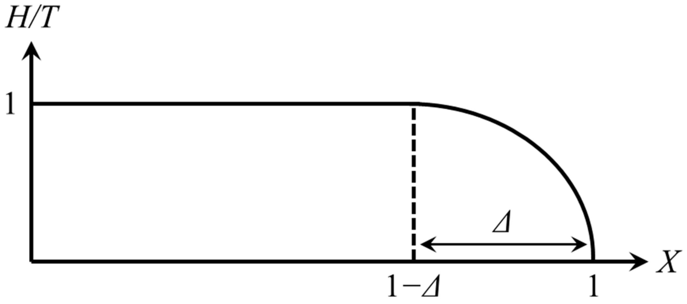
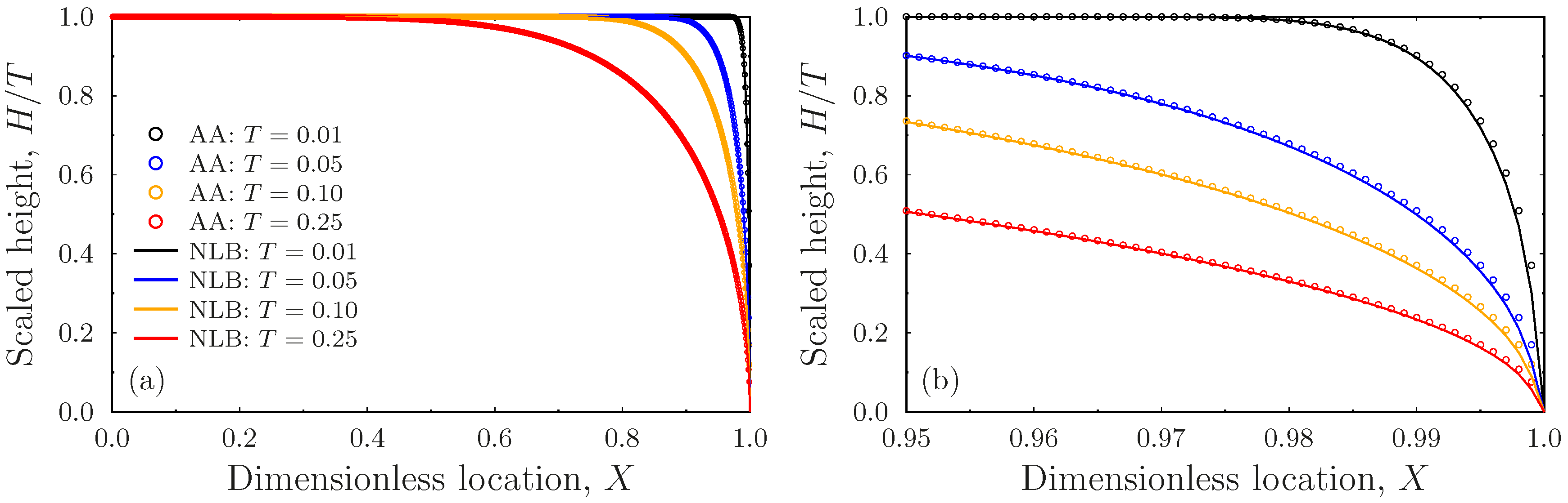
• The linear wave approximation amounts to a constant velocity disturbance traveling from the outlet toward the inlet, where the form is dictated by the singular boundary condition. The discharge associated with this solution turns out to vary linear with time, as expected from the results in [39], while the water table’s profile encapsulates very well the behavior of the nonlinear Boussinesq equation at early times;
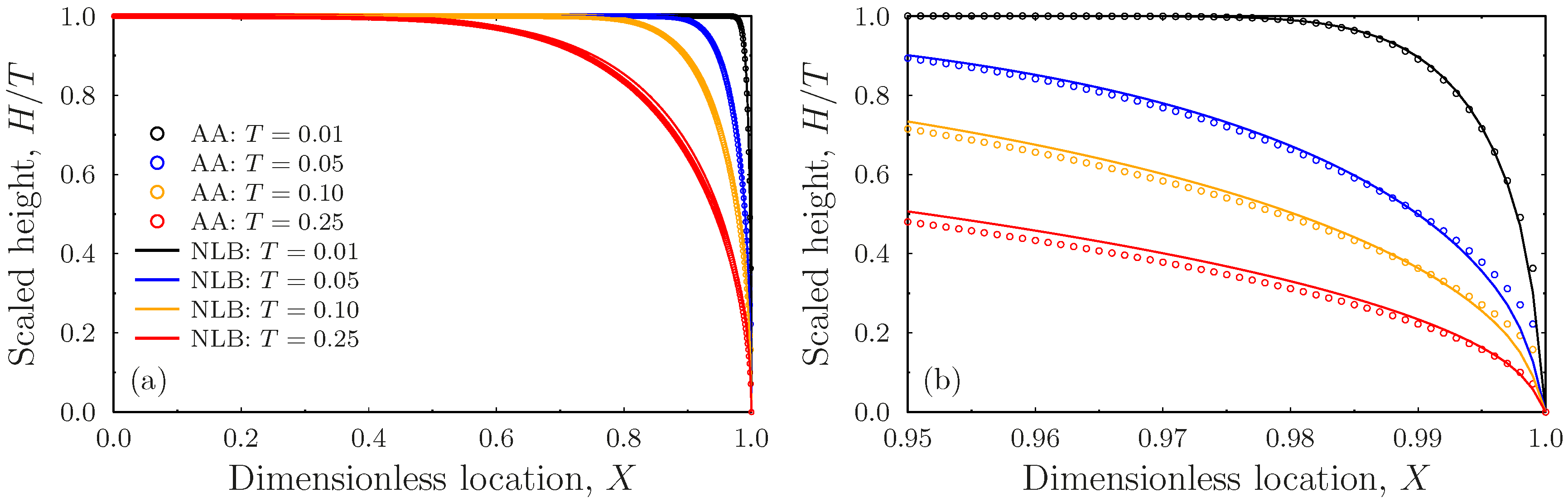
• The self-similarity approximation employs the linearization of an exact self-similarity equation deduced from the Boussinesq equation applicable for early times. This approximate solution also produces a linear discharge rate, although the water table profiles have some visible discrepancies from that of the nonlinear Boussinesq equation. This is due to an outlet boundary behavior, which is somewhat inconsistent with the Boussinesq equation;
• The classical linear approximation of the Boussinesq equation leads to an equation that can be solved using Fourier series. Although the early time asymptotic of the discharge is linear in time, the water table’s profile has significant deviations from that of the Boussinesq equation because of a boundary behavior at the outlet, which is inconsistent with the square-root singularity of the problem. This is characteristic of the linear approximation of the Boussinesq equation. The quadratic approximation of the Boussinesq equation is naturally consistent with the square-root singular behavior of the water table at the outlet; hence, the profiles have relatively small deviations from those of the nonlinear equation. The discharge also turns out to be a linear function of time in this case, although it underestimates by some 10% the slope of the discharge according to the exact nonlinear equation.

The results from this research could be used as benchmarks for numerical modeling and to serve as the basis for further theoretical development in groundwater hydrology with practical importance. For example, the wave’s approximate solution, which describes quite faithfully the solution of the exact nonlinear Boussinesq equation, could be used for validation purposes of numerical schemes treating horizontal and gently inclined aquifers. Plausibly, these ideas could be further exploited to build simple, but effective, models for the more general and interesting case of sloping aquifers. That will be the subject of the future work of these authors.

References

1. Boussinesq, J. Essai sur la theorie des eaux courantes du mouvement nonpermanent des eaux souterraines. Acad. Sci. Inst. Fr. 1877, 23, 252–260. [Google Scholar]
2. Boussinesq, J. Recherches theoriques sur l’ecoulement des nappes d’eau infiltrees dans le sol et sur debit de sources. J. Math. Pures Appl. 1904, 10, 5–78. [Google Scholar]
3. Dupuit, J. Etudes Theoriques et Practiques sur le Mouvement des Eaux dans les Canaux Decouverts et a Travers les Terrains Permeables, 2nd ed.; Dunod: Paris, France, 1863. [Google Scholar]
4. Forchheimer, P. Über die Ergiebigkeit von Brunnen-Anlagen und Sickerschlitzen. Z. Architekt. Ing.-Ver. Hann. 1886, 32, 539–563. [Google Scholar]
5. Wooding, R.A.; Chapman, T.G. Groundwater flow over a sloping impermeable layer: 1. Application of the Dupuit-Forchheimer assumption. J. Geophys. Res. 1966, 71, 2895–2902. [Google Scholar] [CrossRef]
6. Barenblatt, G.I. On some unsteady fluid and gas motions in a porous medium. J. Appl. Math. Mech. 1952, 16, 67–78. [Google Scholar]
7. Polubarinova-Kochina, P.Y. Theory of Ground Water Movement; Princeton University Press: Princeton, NJ, USA, 1962. [Google Scholar]
8. Barenblatt, G.I.; Entov, V.M.; Ryzhik, V.M. Theory of Fluid Flows through Natural Rocks; Kluwer Academic Publishers: Dordrecht, The Netherlands, 1990. [Google Scholar]
9. Chen, Z.X.; Bodvarsson, G.S.; Witherspoon, P.A.; Yortsos, Y.C. An integral equation formulation for the unconfined flow of groundwater with variable inlet conditions. Trans. Porous Media 1995, 18, 15–36. [Google Scholar] [CrossRef]
10. Lockington, D.A.; Parlange, J.Y.; Parlange, M.B.; Selker, J. Similarity solution of the Boussinesq equation. Adv. Water Resour. 2000, 23, 725–729. [Google Scholar] [CrossRef]
11. Parlange, J.Y.; Hogarth, W.L.; Govindaraju, R.S.; Parlange, M.B.; Lockington, D. On an exact analytical solution of the Boussinesq equation. Trans. Porous Media 2000, 39, 339–345. [Google Scholar] [CrossRef]
12. Telyakovskiy, A.S.; Braga, G.A.; Furtado, F. Approximate similarity solutions to the Boussinesq equation. Adv. Water Resour. 2002, 25, 191–194. [Google Scholar] [CrossRef]
13. Pistiner, A. Similarity solution to unconfined flow in an aquifer. Trans. Porous Media 2008, 71, 265–272. [Google Scholar] [CrossRef]
14. Moutsopoulos, N. Solutions of the Boussinesq equation subject to a nonlinear Robin boundary condition. Water Resour. Res. 2013, 49, 7–18. [Google Scholar] [CrossRef]
15. Basha, H.A. Traveling wave solution of the Boussinesq equation for groundwater flow in horizontal aquifers. Water Resour. Res. 2013, 49, 1668–1679. [Google Scholar] [CrossRef]
16. Basha, H.A. Perturbation solutions of the Boussinesq equation for horizontal flow in finite and semi-infinite aquifers. Adv. Water Resour. 2021, 155, 104016. [Google Scholar] [CrossRef]
17. Chor, T.; Ruiz de Zarate, A.; Dias, N.L. A generalized series solution for the Boussinesq equation with constant boundary conditions. Water Resour. Res. 2019, 55, 3567–3575. [Google Scholar] [CrossRef]
18. Chor, T.; Dias, N.L.; Ruiz de Zárate, A. An exact series and improved numerical and approximate solutions for the Boussinesq equation. Water Resour. Res. 2013, 49, 7380–7387. [Google Scholar] [CrossRef]
19. Tzimopoulos, C.; Papadopoulos, K.; Papadopoulos, B.; Samarinas, N.; Evangelides, C. Fuzzy solution of nonlinear Boussinesq equation. J. Hydroinformatics 2022, 24, 1127–1147. [Google Scholar] [CrossRef]
20. Hayek, M. A simple and accurate closed-form analytical solution to the Boussinesq equation for horizontal flow. Adv. Water Resour. 2024, 185, 104628. [Google Scholar] [CrossRef]
21. Tzimopoulos, C.; Samarinas, N.; Papadopoulos, K.; Evangelides, C. Fuzzy Analytical Solution for the Case of a semi-Infinite Unconfined Aquifer. Environ. Sci. Proc. 2023, 25, 70. [Google Scholar] [CrossRef]
22. Ceretani, A.; Falcini, F.; Garra, R. Exact solutions for the fractional nonlinear Boussinesq equation. In Proceedings of the INdAM Workshop on Fractional Differential Equations: Modeling, Discretization, and Numerical Solvers, Singapore, 8 March 2023; Springer Nature: Singapore, 2023. [Google Scholar]
23. Daly, E.; Porporato, A. A note on groundwater flow along a hillslope. Water Resour. Res. 2004, 40, W01601. [Google Scholar] [CrossRef]
24. Barenblatt, G.I. Scaling, Self-Similarity, and Intermediate Asymptotics, 1st ed.; Cambridge Univ. Press: New York, NY, USA, 1996. [Google Scholar]
25. Bear, J. Dynamics of Fluids in Porous Media, 1st ed.; Dover Publications: New York, NY, USA, 1972. [Google Scholar]
26. Gravanis, E.; Sarris, E. A working model for estimating CO2-induced uplift of cap rocks under different flow regimes in CO2 sequestration. Geomech. Energy Environ. 2023, 33, 100433. [Google Scholar] [CrossRef]
27. Telyakovskiy, A.S.; Allen, M.B. Polynomial approximate solutions to the Boussinesq equation. Adv. Water Resour. 2006, 29, 1767–1779. [Google Scholar] [CrossRef]
28. Telyakovskiy, A.S.; Braga, G.A.; Kurita, S.; Mortensena, J. On a power series solution to the Boussinesq equation. Adv. Water Resour. 2010, 33, 1128–1129. [Google Scholar] [CrossRef]
29. Olsen, J.S.; Telyakovskiy, A.S. Polynomial approximate solutions of a generalized Boussinesq equation. Water Resour. Res. 2013, 49, 3049–3053. [Google Scholar] [CrossRef]
30. Dias, N.L.; Chor, T.L.; de Zarate, A.R. A semi-analytical solution of the Boussinesq equation with nonhomogeneous constant boundary conditions. Water Resour. Res. 2014, 50, 6549–6556. [Google Scholar] [CrossRef]
31. Tolikas, P.K.; Sidiropoulos, E.G.; Tzimopoulos, C.D. A simple analytical solution for the Boussinesq one-dimensional groundwater flow equation. Water Resour. Res. 1984, 20, 24–28. [Google Scholar] [CrossRef]
32. Hayek, M. Accurate approximate semi-analytical solutions to the Boussinesq groundwater flow equation for recharging and discharging of horizontal unconfined aquifers. J. Hydrol. 2019, 570, 411–422. [Google Scholar] [CrossRef]
33. Akylas, E.; Koussis, A.D. Response of sloping unconfined aquifer to stage changes in adjacent stream I. Theoretical analysis and derivation of system response functions. J. Hydrol. 2007, 338, 85–95. [Google Scholar] [CrossRef]
34. Beven, K. Kinematic subsurface stormflow. Water Resour. Res. 1981, 17, 1419–1424. [Google Scholar] [CrossRef]
35. Henderson, F.M.; Wooding, R.A. Overland flow and groundwater flow from a steady rainfall of finite duration. J. Geophys. Res. 1964, 69, 1531–1540. [Google Scholar] [CrossRef]
36. Akylas, E.; Gravanis, E.; Koussis, A.D. Quasi-steady flow in sloping aquifers. Water Resour. Res. 2015, 51, 9165–9181. [Google Scholar] [CrossRef]
37. Lighthill, M.J.; Whitham, G.B. On kinematic waves. I. Flood movement in long rivers. In Proceedings of the Royal Society of London A: Mathematical, Physical and Engineering Sciences, 10 May 1955; Volume 229, pp. 281–316. [Google Scholar]
38. Akylas, E.; Koussis, A.D.; Yannacopoulos, A.N. Analytical solution of transient flow in a sloping soil layer with recharge. J. Hydrol. Sci. 2006, 51, 626–641. [Google Scholar] [CrossRef]
39. Gravanis, E.; Akylas, E. Early-time solution of the horizontal unconfined aquifer in the buildup phase. Water Resour. Res. 2017, 53, 8310–8326. [Google Scholar] [CrossRef]
40. Moutsopoulos, K.N. The analytical solution of the Boussinesq equation for flow induced by a step change of the water table elevation revisited. Trans. Porous Med. 2010, 85, 919–940. [Google Scholar] [CrossRef]
41. Verhoest, N.E.; Troch, P.A. Some analytical solutions of the linearized Boussinesq equation with recharge for a sloping aquifer. Water Resour. Res. 2000, 36, 793–800. [Google Scholar] [CrossRef]
42. Jiang, Q.; Tang, Y. A general approximate method for the groundwater response problem caused by water level variation. J. Hydrol. 2015, 529, 398–409. [Google Scholar] [CrossRef]
43. Lockington, D.A. Response of unconfined aquifer to sudden change in boundary head. J. Irrig. Drain. Eng. 1997, 123, 24–27. [Google Scholar] [CrossRef]
44. Chapman, T.G. Steady recharge-induced groundwater flow over a plane bed: Nonlinear and linear solutions. In Proceedings of the MODSIM 2003 International Congress on Modelling and Simulation, Townsville, Australia, 14–17 July 2003. [Google Scholar]
45. Childs, E.C. Drainage of groundwater resting on a sloping bed. Water Resour. Res. 1971, 7, 1256–1263. [Google Scholar] [CrossRef]
46. Brutsaert, W.; John, L.N. Regionalized drought flow hydrographs from a mature glaciated plateau. Water Resour. Res. 1977, 13, 637–643. [Google Scholar] [CrossRef]
47. Arfken, G.B. Mathematical Methods for Physicists; Elsevier Academic Press: Cambridge, MA, USA, 2005. [Google Scholar]
48. Gratton, J.; Minotti, F. Self-similar viscous gravity currents: Phase-plane formalism. J. Fluid Mech. 1990, 210, 155–182. [Google Scholar] [CrossRef]
49. Van Dyke, M. Perturbation Methods in Fluid Mechanics; Parabolic Press: Stanford, CA, USA, 1975. [Google Scholar]
50. Chapman, T.G. Modeling groundwater flow over sloping beds. Water Resour. Res. 1980, 16, 1114–1118. [Google Scholar] [CrossRef]
51. Chapman, T.G. Comment on: The unit response of groundwater outflow from a hillslope. Water Resour. Res. 1995, 31, 2376–2777. [Google Scholar] [CrossRef]
52. Koussis, A.D.; Lien, L.T. Linear theory of subsurface stormflow. Water Resour. Res. 1982, 18, 1738–1740. [Google Scholar] [CrossRef]
53. Koussis, A.D. A linear conceptual subsurface storm flow model. Water Resour. Res. 1992, 28, 1047–1052. [Google Scholar] [CrossRef]
54. Basha, H.A.; Maalouf, S.F. Theoretical and conceptual models of subsurface hillslope flows. Water Resour. Res. 2005, 41, W07018. [Google Scholar] [CrossRef]
Figure 1. Section of horizontal soil layer under constant recharge and constant hydraulic conditions.
Water 16 01031 g001
Figure 2. Schematic representation of the water profile during the early filling phase of the horizontal aquifer (in dimensionless variables). The action of the discharge, in the form of the profile in the outlet area of the aquifer, has a range (Δ), starting from zero and increasing with time, resembling a wave.
Water 16 01031 g002
Figure 3. (a) Water profiles during the early buildup phase of the horizontal aquifer (in dimensionless variables). Continuous lines: numerical solutions of the nonlinear Boussinesq equation. Dotted lines: the detailed approximation solutions according to (35). The curves correspond to dimensionless times T = 0.01, 0.05, 0.10, and 0.25, starting from the rightmost curve. (b) These curves are focused near the outlet area of the aquifer.
Water 16 01031 g003
Figure 4. (a) Water profiles during the early buildup phase of the horizontal aquifer (in dimensionless variables). Continuous lines: numerical solutions of the nonlinear Boussinesq equation. Dotted lines: the linearized self-similarity solutions given by the relations in (57) and (59). The curves correspond to dimensionless times T = 0.01, 0.05, 0.10, and 0.25, starting from the rightmost curve. (b) The curves focused near the outlet area of the aquifer.
Water 16 01031 g004
Figure 5. Water profiles during the early filling phase of the horizontal aquifer (in dimensional variables). Continuous lines: numerical solutions of the nonlinear Boussinesq equation. Dotted lines: the solutions of the linear approximation models in relations (75) and (76). The curves correspond to dimensionless times T = 0.01, 0.05, 0.10, and 0.25, starting from the rightmost curve.
Water 16 01031 g005
Figure 6. (a) Water profiles during the early filling phase of the horizontal aquifer (in dimensional variables). Continuous lines: numerical solutions of the nonlinear Boussinesq equation. Dotted lines: the solutions of the quadratic approximation model of relations in (84). The curves correspond to dimensionless times T = 0.01, 0.05, 0.10, and 0.25, starting from the rightmost curve. (b) The discharge of the quadratic approximation model as a function of time during the early filling phase.
Water 16 01031 g006
Figure 7. (a) The curves in Figure 6 correspond to dimensionless times T = 0.5, 1.0, 1.5, and 2.0, from the bottom up. (b) The discharges from the numerical solution of the Boussinesq equation (solid line) and the solution of the quadratic model (dotted line) at time T = 2.
Water 16 01031 g007
Disclaimer/Publisher’s Note: The statements, opinions and data contained in all publications are solely those of the individual author(s) and contributor(s) and not of MDPI and/or the editor(s). MDPI and/or the editor(s) disclaim responsibility for any injury to people or property resulting from any ideas, methods, instructions or products referred to in the content.