A Feature Selection Method Based on Relief Feature Ranking with Recursive Feature Elimination for the Inversion of Urban River Water Quality Parameters Using Multispectral Imagery from an Unmanned Aerial Vehicle

Abstract

The timely monitoring of urban water bodies using unmanned aerial vehicle (UAV)-mounted remote sensing technology is crucial for urban water resource protection and management. Addressing the limitations of the use of satellite data in inferring the water quality parameters of small-scale water bodies due to their spatial resolution constraints and limited input features, this study focuses on the Zao River in Xi’an City. Leveraging UAV multispectral imagery, a feature selection method based on Relief Feature Ranking with Recursive Feature Elimination (Relief F-RFE) is proposed to determine the quality parameters of the typical urban pollution in water (dissolved oxygen (DO), total nitrogen (TN), turbidity, and chemical oxygen demand (COD). By constructing a potential feature set and utilizing optimal feature combinations, inversion models are developed for the four water quality parameters using three machine learning (ML) algorithms (Random Forest (RF), Support Vector Regression (SVR), Light Gradient Boosting Machine (LightGBM). The inversion accuracies of the different models are compared, and the spatial distribution of the four water quality parameters is analyzed. The results show that the models constructed based on UAV-based multispectral remote sensing imagery perform well in inferring the water quality parameters of the Zao River. The SVR algorithm, based on Relief F-RFE feature selection, achieves a higher accuracy, with RMSE values of 7.19 mg/L, 1.14 mg/L, 3.15 NTU, and 4.28 mg/L, respectively. The methods and conclusions of this study serve as a reference for research on the inversion of water quality parameters in urban rivers.

1. Introduction

Rivers, as crucial ecological components of urban areas, consistently influence and constrain the survival and development of cities [1]. Throughout the process of urbanization, human activities, global warming, and extreme weather events all impact the water quality and circulation of urban rivers, leading to the increasingly severe pollution of urban water bodies [2,3,4]. Water quality monitoring forms the fundamental basis of water quality assessments and pollution prevention, an essential prerequisite for effectively managing urban water environments. A timely and comprehensive understanding of the trends in water pollution is key to effectively safeguarding water resources [5]. Traditional water quality monitoring methods, such as on-site sampling and laboratory analysis, are associated with high data acquisition costs, low processing efficiency, and an inability to achieve comprehensive pollution monitoring across large-scale watersheds [6]. In contrast, spaceborne sensors can offer long-time series of high-frequency remote sensing images, serving as a reliable means of monitoring regional water quality [7,8]. They rely on the relationship between the spectral reflectance and quality parameters of water [9]. Previous studies predominantly utilized satellite-based platforms for monitoring, including the Landsat Thematic Mapper [10], Sentinel-2 [11], Landsat Operational Land Imager (OLI) [12], and medium-resolution imaging spectrometers [13]. However, due to drawbacks such as low spatial resolution, long revisit cycles, and susceptibility to cloud cover interference, satellite remote sensing does not yield ideal monitoring results for most small and widely dispersed urban water bodies. With the continuous development of near-surface remote sensing technology, unmanned aerial vehicle (UAV) surveying can effectively complement the limitations of the two water quality monitoring methods mentioned above, offering significant advantages in monitoring small-area water pollution. This boasts advantages such as flexibility in its movement, convenient operation, high speeds, low costs, high spatial–temporal resolution, and the ability to determine water quality changes within a relatively short revisit cycle, presenting significant development potential for the quantitative analysis of water quality [14]. Zhu et al. utilized UAV multispectral data and quasi-synchronous water quality sampling data to establish single-band water quality inversion models for water quality parameters such as dissolved oxygen (DO) and total nitrogen (TN) [15]. McEliece R et al. inverted chlorophyll-a (Chl-a) and turbidity in nearshore areas by constructing algorithms based on the differences in the measured spectral reflectance of each water quality parameter in UAV multispectral imagery, demonstrating that UAV multispectral sensors can be used to quantify water quality parameters [16].

In the past, statistical methods were primarily used, making it difficult to accurately quantify and monitor water quality. With the rapid development of artificial intelligence, more research has applied machine learning (ML) methods to monitor water quality using remote sensing [17,18], including Random Forest (RF), Support Vector Regression (SVR), Light Gradient Boosting Machine (LightGBM), and other ML algorithms. In contrast, ML can more precisely construct the linear and nonlinear relationships between the spectral information of images and ground measurement data in complex urban water environments [19]. The estimation results of the suspended sediment concentration prediction model constructed by Fang et al. show that compared to linear regression, support vector machines, and artificial neural network models, the RF model has the highest inversion accuracy [20]. Yan et al. utilized the SVR model to construct TN and Total Organic Carbon (TOC) models, with validation period R² values of 0.78 and 0.83, respectively, demonstrating their good simulation and estimation capabilities [21]. Xiang et al. used Temporal Convolutional Networks (TCNs), LightGBM, and four single features to make a quadratic decomposition-based water quality prediction model, demonstrating that LightGBM is suitable for handling the low-frequency components in information, making the model more flexible [22]. Yan et al. conducted a comparative analysis of the technical characteristics and accuracy of several inversion models, including RF, and constructed an optimal water quality parameter inversion model, discussing the influence of different inversion methods on the prediction of water quality parameters [23].

Due to factors such as spectral resolution and spatial resolution, optical imagery is susceptible to phenomena such as spectral confusion (same spectrum, different substances) and substance confusion (same substance, different spectra) [24]. Furthermore, most inversion methods for water quality parameters involve comparative analyses of ML algorithms, with limited consideration given to the potential impact of their features on the inversion models of urban water body water quality parameters. This oversight neglects the importance of feature selection and the issue of feature redundancy. Currently, some scholars are conducting research on feature selection, with the most commonly used methods being filter-based algorithms and wrapper-based algorithms. Many scholars optimize algorithms’ features based on methods such as SVM-RFE [25,26] and RF-RFE [27,28]. Marwa et al. proposed a multi-objective hybrid filter–wrapper evolutionary algorithm for the high-dimensional feature construction of data, which combines the advantages of both filter and wrapper algorithms [29]. This approach showed significant effectiveness in eliminating redundant features. Xiang et al. compared the Relief F-RFE feature selection algorithm with the single Relief F and RFE algorithms, demonstrating that it exhibits a more balanced overall performance in feature selection for hyperspectral image classification [30].

Based on this research, this study focuses on a section of the Zao River in Xi’an, Shaanxi Province, China. High-resolution multispectral data were acquired using unmanned aerial vehicles (UAVs). Simultaneously, water quality data from the study area were obtained on-site, and indoor water quality testing was performed. Subsequently, a potential feature set was constructed for four types of water quality parameters (DO, TN, turbidity, COD). The Relief F-RFE algorithm was used to gradually reduce and determine the optimal number of model features. Then, inversion models were constructed based on those optimal feature combinations using RF, SVR, and LightGBM. Finally, the spatial distribution patterns of different parameter concentrations were analyzed. By comparing the results of three types of ML inversion with and without feature selection, this study effectively demonstrates the advantages of Relief F-RFE feature selection in the inversion of water quality parameters using UAV multispectral data. This provides valuable insights for research on water quality inversion methods in urban rivers.

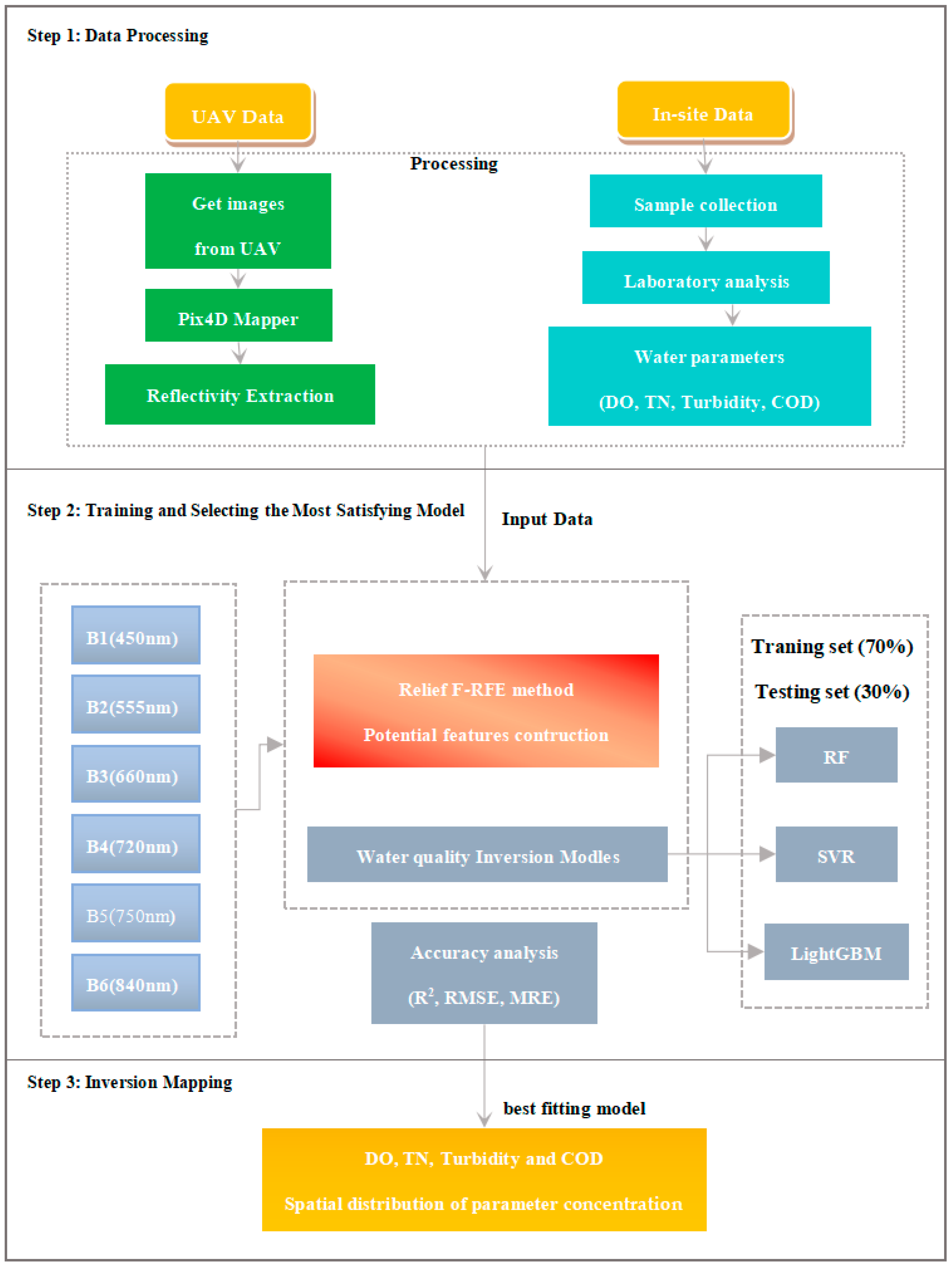
2. Materials and Methods

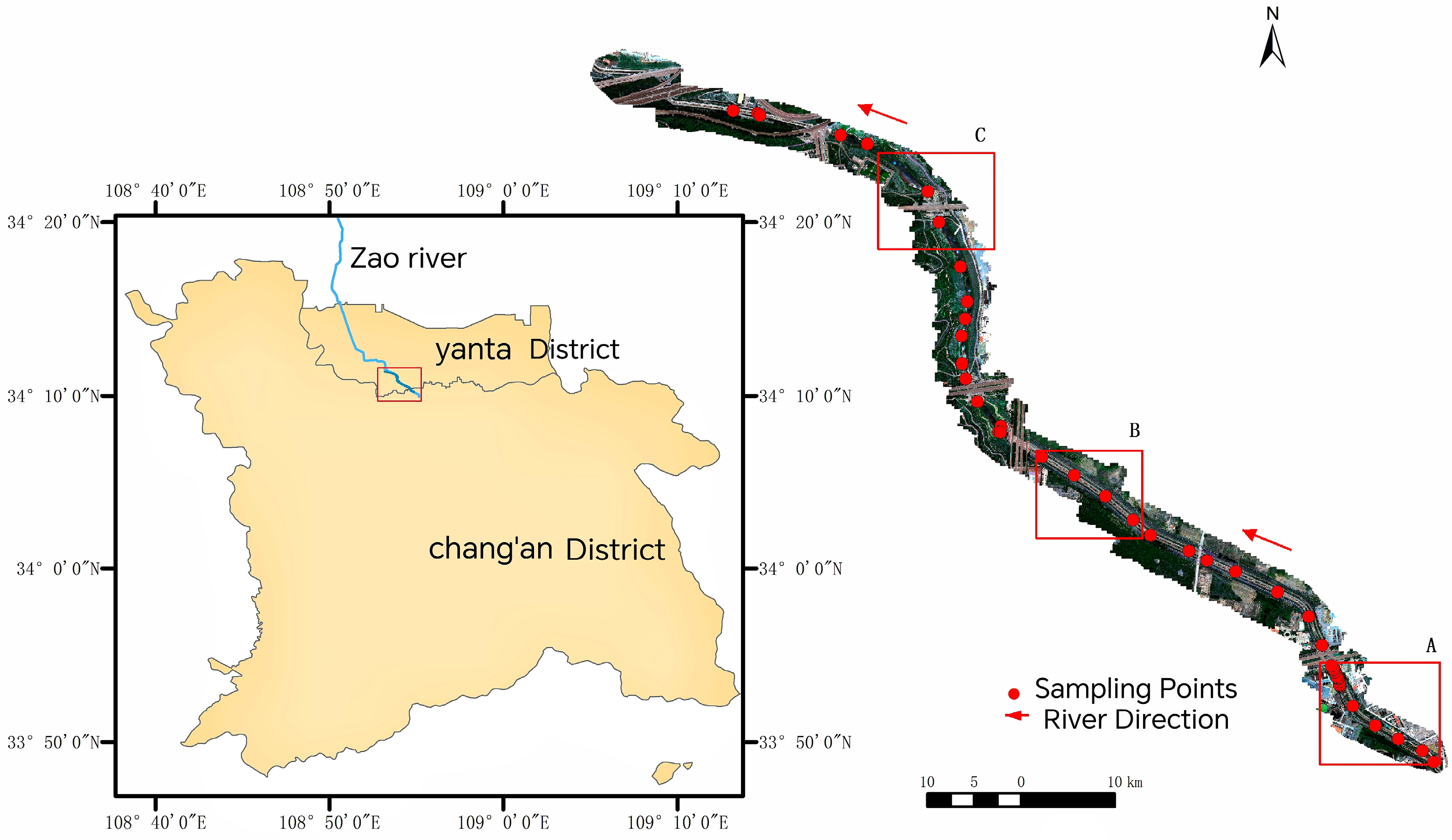
2.1. Study Area

The Zao River, as one of the tributaries of the Wei River, is one of the five major flood diversion systems in the urban area of Xi’an, which include the Chan River, Ba River, Zao River, Caoyun River, and Xingfu River. It is a typical small urban river with a total length of 35.85 km, an in-city length of 12.6 km, and an average annual runoff of 47 million cubic meters. On the day of sampling, the actual water depth measured was 2.70 m. The river channel is narrow, with a width ranging from 3 m to 10 m and no upstream inflow as supplementation. Due to the addition of sewage or treated effluent to the river, its ecological improvement faces significant challenges [31]. Currently, the water quality of the Zao River remains unstable (Xi’an Municipal Ecology and Environment Bureau, 2021).

The study area is located at the junction of the Yanta District and Chang’an District in Xi’an City, Shaanxi Province. The total length of the analyzed section of the river is 9 km. Its geographical coordinates are from 108°50′ E to 108°55′ E longitude and 34°10′ N to 34°24′ N latitude. In the upstream region of the study area, there are mainly parks, factories, and centralized sewage outlets. The midstream region, on both sides of the river, is mainly parks, green spaces, and rubber tracks. The downstream region, on both sides of the river, is green park spaces. The entire study area was divided into segments comprising parks, factories, and residential areas. In the study area, 44 water quality sampling points were selected, as depicted in Figure 1. Based on the ecological environment of the river, from upstream to downstream, three sensitive water quality areas were selected for study and analysis. These areas are an upstream area (Area A), a midstream area (Area B), and a downstream area (Area C) [32,33].

2.2. Data

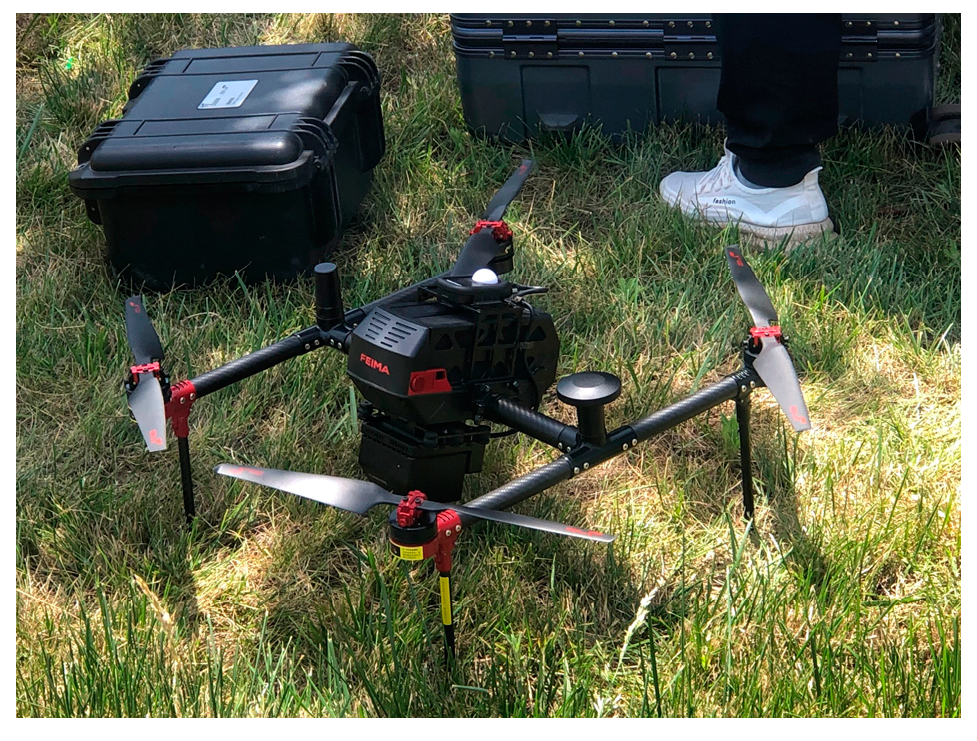
2.2.1. UAV Data and Preprocessing

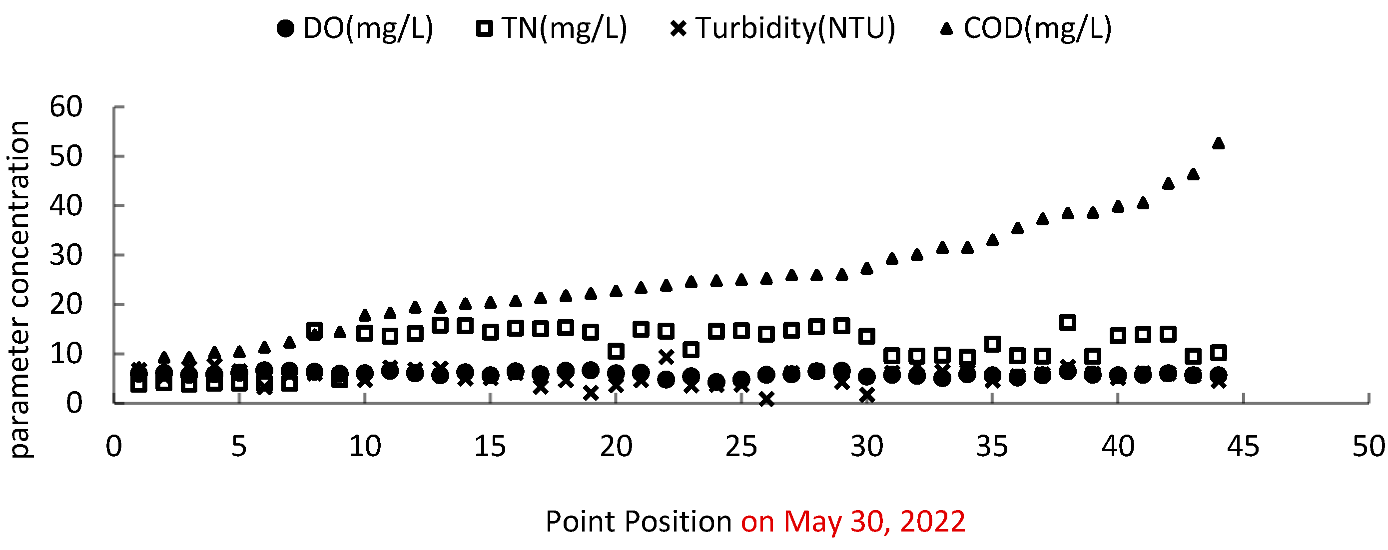
The data sources for this study include multispectral aerial imagery obtained from UAV flights and in situ water quality sample data synchronously collected in the field. The UAV data were acquired using a FlyHawk UAV (Figure 2), equipped with an MS600 sensor for multispectral data collection. The course overlap degree was set at 80%, and the side overlap degree was set at 70%. The camera comprised six channels, providing images of blue (450 nm), green (555 nm), red (660 nm, 720 nm, 750 nm), and near-infrared (840 nm) bands simultaneously. The specifications of the UAV used are shown in

Table 1. Specifications for the FlyHawk UAV.

Specifications	Numerical Value
empty weight	2.60 kg
loading capacity	1.20 kg
boundary dimension	$\mathrm{spread} 495 \mathrm{mm} \times$ $442 \mathrm{mm}\times$279 mm
	$\mathrm{fold} 495 \mathrm{mm}\times$$442 \mathrm{mm}\times 143$ mm
maximum flying speed	20 m/s
hover time	60 min
operating temperature	−20 °C~45 °C

, and its main parameter information and band details are provided in

Table 2. UAV load parameters and band information.

Project	Numerical Value	Band	Wavelength (nm)
sensor parameter	CMOS: 1/3” global shutter	B1	450 ± 35
sensor size	4.80 mm × 3.60 mm	B2	555 ± 25
resolution ratio	1280 × 960	B3	660 ± 22.5
focal length	5.20 mm	B4	720 ± 10
field angle	HFOV: 49.60°, HFOV: 38°	B5	750 ± 10
aperture	F/2.20	B6	840 ± 30

. The UAV imagery was acquired on 30 May 2022, at noon (12:00 p.m.), from a flight altitude of 120 m.

Obtain pre-calibrated image data and use Pix4D 4.5.6 software to generate orthomosaic images for six bands. Then, perform overall registration on the already radiometrically calibrated and orthomosaic single-band images of the study area to generate the final image. Import the data into ENVI and draw 3 × 3 ROIs centered on the pixels that correspond to points of interest. Use the average band reflectance values of the ROIs as the raw data for model construction.

2.2.2. On-Site Data

Before conducting field data collection, 44 representative sampling points were evenly distributed across the flight path of an unmanned aerial vehicle (UAV), taking into account the sewage outlet, historical data and expert recommendations. While the UAV captured imagery, water samples were collected simultaneously. The actual sample collection was carried out five times 0.20 m below the water’s surface at each sampling point. Refer to the industry standard ”Technical Specifications for Water Quality Sampling” (No. HJ494-2009) [34], a minimum of 150 mL was collected for each type of water quality sample, with a total of four types of water quality samples collected, along with additional backup samples. This totaled to 850 mL collected per sample point. The collected water samples were then analyzed in the laboratory using detection instruments and reagents to obtain actual water quality data.

Water quality parameters can be categorized into optical and non-optical parameters. Optical water quality parameters include chlorophyll-a (Chl-a), turbidity, and total suspended matter (TSM). These parameters exhibit distinct spectral characteristics and are directly related to the light spectrum. On the other hand, non-optical water quality parameters, such as dissolved oxygen (DO), total phosphorus (TP), total nitrogen (TN), and chemical oxygen demand (COD), do not have purely optical properties.

This study selects DO, TN, turbidity, and COD as the parameters for inversion, which can best reflect the water environment of the Zao River. Among these, DO is an indicator reflecting the self-purification ability of water bodies. Temperature is the primary factor influencing the dissolved oxygen content in water. Generally, the lower the temperature, the higher the dissolved oxygen content in water. Severe water pollution leads to lower DO levels [35]. TN represents the total amount of inorganic and organic nitrogen in water and is commonly used to describe the degree of eutrophication in lake water bodies [36]. Turbidity, an optical effect, indicates the degree to which light passing through a layer of water is obstructed. The measurement of turbidity is one of the most important tests for measuring water pollution [37]. COD measures the quantity of reducible substances in the water that need to be oxidized using chemical methods. It can reflect the pollution level of organic and inorganic oxidizable substances in the water [38].

The statistical information on the four water quality parameters is presented in

Table 3. Statistical information table of water quality parameters (DO, TN, turbidity, COD).

Index	DO/(mg/L)	TN/(mg/L)	Turbidity/(NTU)	COD/(mg/L)
Minimum value	4.30	3.84	0.93	7.25
Maximum value	6.70	16.32	9.43	52.66
Mean value	5.91	11.50	5.47	25.14
Standard Deviation	0.53	4.12	1.68	10.76
Coefficient of Variation	0.09	0.36	0.31	0.43

. It was observed that TN and COD concentrations had large standard deviations of 4.12 mg/L and 10.76 mg/L, respectively, indicating unstable water quality conditions. Furthermore, the statistical analysis of water quality concentrations at various sampling points along the Zao River, from upstream to downstream, is illustrated in Figure 3. DO and turbidity concentrations exhibit relatively stable variations overall. However, COD concentrations show a continuous upward trend from upstream to downstream. The TN concentration values are generally high, all exceeding 2 mg/L, which, according to the national standard “Surface Water Environmental Quality Standard GB3838-2002”, correspond to Class V water quality, indicating poor water quality [39].

2.3. Methodology

2.3.1. Potential Feature Dataset Construction

The spectral characteristics of water bodies represent their comprehensive response to the spectral behavior of their water components. Therefore, constructing a model feature set is crucial. In this study, six bands of multispectral data were used to construct a latent feature set, as seen in

Table 4. Selection of potential features.

Feature Type	Variable Name	Formula	Quantity (PCS)
Single-band Feature	Band (i)	B (i)	6
Transformed-band Feature	Ln (i)	$\mathrm{Ln} (B_i$)	6
Two-band Combination Feature	NDI (i,j)	$\left(B_i-B_j\right)/\left(B_i+B_j\right)$	15
	DI (i,j)	$B_i-B_j$	15
	RI (i,j)	$B_i/B_j$	30
Total			72

. Its selection is divided into three categories, single-band features, transformed band features, and combined band features, for a total of 72 features. Feature selection was performed based on this latent feature set and input into the model.

2.3.2. Relief F-RFE Feature Optimization Algorithm

To enhance the accuracy and predictive precision of ML algorithms, we employ a combined approach of filter-based and wrapper-based feature selection. This includes three main steps: (1) an analysis of the correlation between features of different types (single-band, transformed band, and combined band), (2) Relief F-RFE filter-based feature selection, and (3) a recursive feature elimination algorithm for feature optimization. The ultimate goal is to identify the critical features for the inversion of our identified water quality parameters. This method aims to reduce the decrease in classification accuracy caused by information redundancy while improving the computational efficiency of the classification model.

The core idea of the Relief F-RFE filter-based algorithm is that it evaluates the classification contribution of candidate features by computing the differences between instances of different classes. If a feature in the feature set results in a larger distance between instances of different classes compared to instances of the same class, it indicates that this feature is beneficial for classification. Therefore, its weight is increased. Conversely, if the distance between instances of different classes is smaller than instances of the same class, the weight of the feature is decreased. Finally, the average of n iterations’ computation results is taken as the final weight of each feature. The Relief F-RFE weight calculation formula for the four types of parameters is shown as follows [40]:

$$\omega \left(A_i\right)=\omega \left(A_i\right)-\frac{1}{nk}{{\displaystyle \sum }}_{h\in H}\left|R_i-h_i\right|+\frac{1}{nk}{{\displaystyle \sum }}_{m\in M}\left|R_i-h_i\right|,$$

(1)

In the formula, $\omega \left(A_i\right)$ denotes the weight value of feature $i$, ${{\displaystyle \sum }}_{h\in H}\left|R_i-h_i\right|$ is the $k$ the sum of the distances between the nearest neighbor samples of the same kind and the $R$ samples on the feature, and ${{\displaystyle \sum }}_{m\in M}\left|R_i-h_i\right|$ represents the $k$ is the sum of the distances between the nearest neighbor samples and sample $R$ on feature $i$.

The recursive feature elimination (RFE) algorithm is a feature selection method that uses the wrapper approach. Its core idea involves iteratively training the model, removing the least important features from each run’s results, and recursively repeating this process with the remaining features until the desired number of features is achieved.

2.3.3. Modeling

The Random Forest (RF) model extracts multiple bootstrap samples from the original dataset for decision tree modeling, and then combines multiple decision trees for prediction, and finally aggregates the predictions through voting to obtain a final prediction result. In the process of modeling with RF, improving the model’s prediction accuracy can be achieved by optimizing two important custom parameters, namely, the split attribute value m for each internal split node of a single decision tree and the number of trees n in the forest. By setting different numbers of decision trees, different errors are obtained, and the value of n corresponding to a stable state of error change is selected as the final value. In this study’s model construction, m was set to 2, the range of n was from 70 to 200, with a step size of 10, and the final value was set at 100.

Support Vector Regression (SVR) is a non-probabilistic algorithm that maps data to a high-dimensional space using a kernel function. Parameter tuning is an important process in SVR. In this study, random search is used, with the algorithm employing a linear kernel function (poly) with a degree of 3. The seed for the pseudo-random number generator used when shuffling the data (random_state) is set to 0.

The core principle of the Light Gradient Boosting Machine (LightGBM) algorithm is to make predictions through iteratively training multiple decision trees. Each tree is trained based on the residuals of previous trees, gradually reducing prediction errors. In this algorithm, the objective function is set to regression, and the boosting type is set to Gradient Boosting Decision Tree (GBDT). The learning rate is set to 0.1, and subsample and colsample_bytree are set to 0.80.

The datasets for the RF, SVR, and LightGBM models are constructed in a 7:3 ratio of training to validation. The data processing workflow is depicted in Figure 4.

2.4. Accuracy Evaluation

The water quality parameter inversion models are evaluated for their accuracy using $R^2$, Root Mean Square Error ($RMSE$), and Mean Relative Error ($\mathrm{M}RE$). $R^2$ represents the degree to which the independent variable explains the dependent variable, with higher values indicating better model fitting. $RMSE$ is used to measure the deviation between the observed values and true values, reflecting the actual error of the prediction. A smaller number for this evaluation metric indicates higher model accuracy. $\mathrm{M}RE$ is used to indicate the accuracy of the prediction results. The specific formulas are as follows:

$$R^2=\frac{{{\displaystyle \sum }}_{i=1}^n{\left(y_i^{estimated}-{\overline{y}}^{mean}\right)}^2}{{{\displaystyle \sum }}_{i=1}^n{\left(y_i^{measure}-{\overline{y}}^{mean}\right)}^2},$$

(2)

$$RMSE=\sqrt{\frac{{{\displaystyle \sum }}_{i=1}^n{\left(y_i^{estimated}-\overline{y_i^{measure}}\right)}^2}{n}},$$

(3)

$$\mathrm{M}RE=\frac{1}{n}{{\displaystyle \sum }}_1^n\left(\frac{|y_i^{measure}-y_i^{estiamted}|}{y_i^{measure}}\right)\times 100\%,$$

(4)

In these equations, $y_i^{estiamted}$ represents the model-predicted value, $y_i^{measure}$ represents the measured value of the model, ${\overline{y}}^{mean}$ represents the mean of the measured values at the sample points, and n represents the number of samples.

3. Results

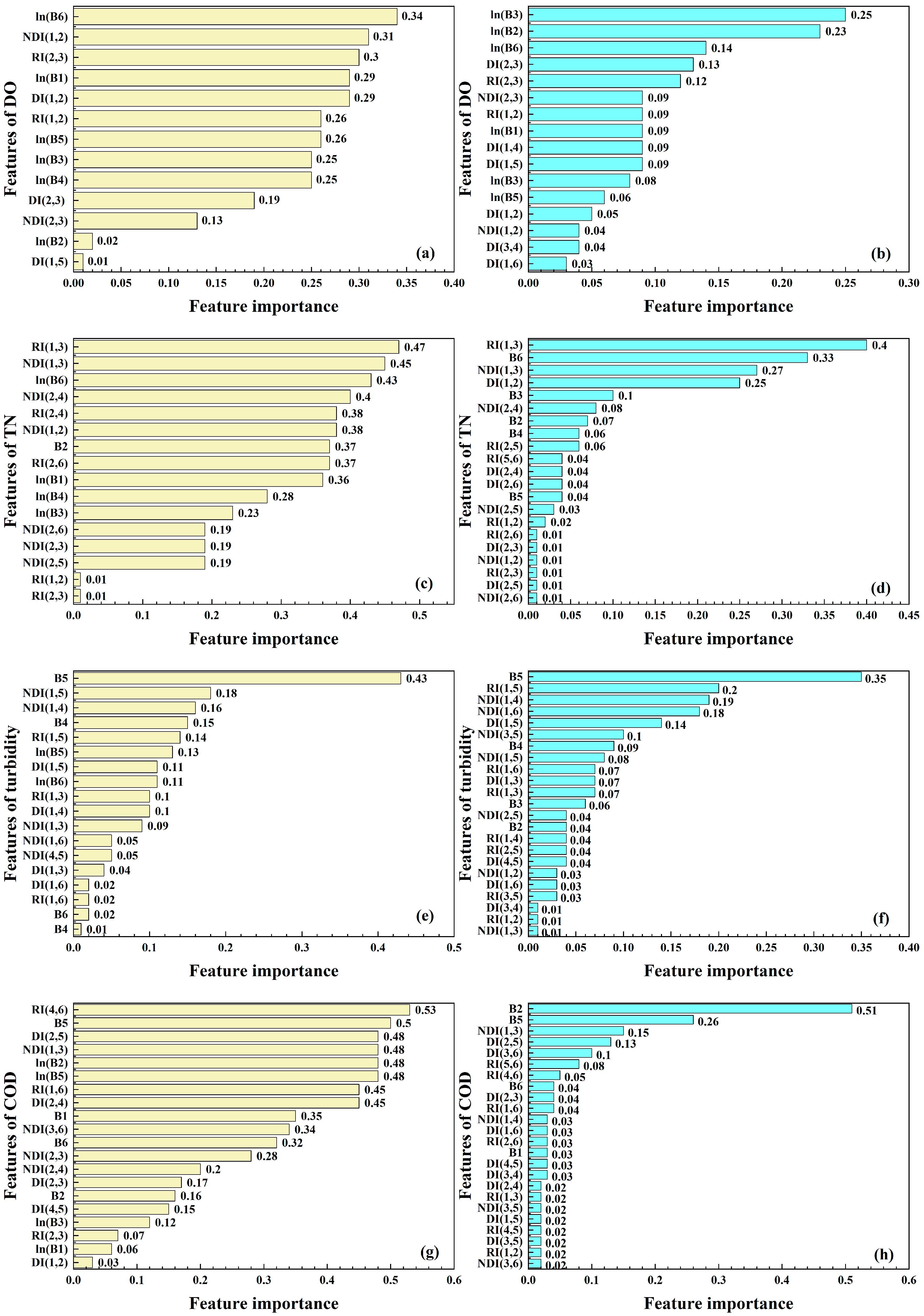
3.1. Feature Optimization Results

This study employed the Relief F-RFE algorithm for the feature selection of a potential feature set. Its specific results are presented in Figure 5. Of the optimal feature variables for DO concentration inversion, the combination feature constructed based on bands B1, B2, and B3 (as shown in (b) of the figure) accounts for 87.50% of all the parameter’s features. Compared to (a), the importance of logarithmic indices and difference indices is more significant here. In the feature selection results for TN concentration, the combination feature mainly relies on the green-edged band B2. Additionally, of the top five features in (d), the red-edged band B3 predominates. In the optimal feature set for turbidity inversion, the combination feature constructed from the red bands B4 and B5 accounts for a relatively high proportion of all features. Combining figures (e) and (f), regardless of whether the Relief F-RFE feature selection algorithm is used, the red bands are important for turbidity inversion. This finding is generally consistent with other researchers’ results (Fang et al., 2019) [20]. In the analysis of COD concentration’s importance, its combination feature of bands generally accounts for a large proportion of the feature set. In comparison to (g), band B2 in Figure (h) exhibits more significance than all other features.

In summary, logarithmic indices play a critical role in determining DO concentrations. Combination features composed of bands are crucial for TN and COD concentration inversions. Red-edged bands are predominant in turbidity concentration inversions.

According to the importance-based band-sorting chart of the four water quality parameters, it can be observed that the Relief F-RFE feature optimization method selects the best feature bands (including transformed and combined bands). These selected bands are then applied to RF, SVR, and LightGBM ML algorithms for modeling. The important bands obtained after feature optimization overlap, to a certain extent, with those obtained directly by applying the ML algorithms without feature optimization. Furthermore, bands with higher importance scores demonstrate increased involvement in these algorithms after feature optimization, for instance, in the case of the DO parameter, with feature bands ln(B6) and RI (2,3); for the TN parameter, with feature bands RI (1,3) and NDI (1,3); for the turbidity parameter, with feature bands B5 and NDI (1,4); and for the COD parameter, with feature bands B5, DI (2,5), and NDI (1,3). This indicates that utilizing the Relief F-RFE feature optimization method for feature selection is suitable for water quality inversions of unmanned aerial vehicle multispectral imagery.

3.2. Comparison Analysis of Models

We first performed feature selection based on the Relief F-RFE algorithm and then input its selected features into the RF, SVR, and LightGBM algorithms to invert four parameters: DO, TN, turbidity, and COD. Additionally, to compare the advantages of Relief F-RFE feature selection, we did not conduct feature selection. Instead, we directly input all features into the RF, SVR, and LightGBM algorithms to invert the four parameters. The results are shown in detail in

Table 5. Inversion results of three types of machine learning models (RF, SVR, LightGBM).

Water Quality Type	Retrieval Model	R2	RMSE	MRE%	Retrieval Model	R2	RMSE	MRE%
DO	RF	0.55	19.13 mg/L	7.26	Relief F-RFE-RF	0.71	10.26 mg/L	4.04
	SVR	0.60	13.55 mg/L	4.52	Relief F-RFE-SVR	0.80	7.19 mg/L	2.68
	LightGBM	0.45	17.82 mg/L	8.23	Relief F-RFE-LightGBM	0.67	14.60 mg/L	6.83
TN	RF	0.67	12.27 mg/L	9.22	Relief F-RFE-RF	0.82	6.17 mg/L	6.91
	SVR	0.67	9.34 mg/L	5.56	Relief F-RFE-SVR	0.96	1.14 mg/L	2.32
	LightGBM	0.35	10.45 mg/L	6.69	Relief F-RFE-LightGBM	0.74	4.80 mg/L	5.49
Turbidity	RF	0.54	15.69 NTU	9.26	Relief F-RFE-RF	0.77	10.29 NTU	7.36
	SVR	0.60	13.25 NTU	6.29	Relief F-RFE-SVR	0.84	3.15 NTU	4.92
	LightGBM	0.43	16.88 NTU	9.65	Relief F-RFE-LightGBM	0.73	12.60 NTU	9.05
COD	RF	0.60	19.58 mg/L	11.12	Relief F-RFE-RF	0.84	10.38 mg/L	7.12
	SVR	0.62	11.38 mg/L	5.55	Relief F-RFE-SVR	0.86	4.28 mg/L	3.85
	LightGBM	0.43	12.66 mg/L	5.87	Relief F-RFE-LightGBM	0.70	11.10 mg/L	4.07

.

Based on Table 5, it can be observed that the modeling accuracy of the DO, TN, turbidity, and COD parameters and the fitting performance of the RF, SVR, and LightGBM algorithms constructed using Relief F-RFE are better. TN’s R² value can be increased by up to 0.39. Turbidity’s RMSE can be reduced by up to 10.1, indicating that the model’s accuracy effectively improves with the inclusion of Relief F-RFE feature selection. Additionally, the MRE of DO and COD decreases by 3.22% and 4%, respectively, suggesting an improvement in the accuracy of the model’s predictions. The results indicate that the modeling accuracy of the three ML algorithms is improved, after applying the Relief F-RFE method, compared to directly using the three ML algorithms for modeling. In situations with limited samples, excessive features can degrade the performance of ML algorithms without a feature selection component. Overall, the SVR algorithm outperforms the RF and LightGBM algorithms. Previous studies showed that SVR shows many unique advantages in solving small-capacity samples and nonlinear and high-dimensional regression problems, which is consistent with our results [41]. Among all the models, the inversion model for the TN parameter based on the Relief F-RFE-SVR method achieves the highest accuracy, with R², RMSE, and MRE values of 0.96, 1.14 mg/L, and 2.32%, respectively.

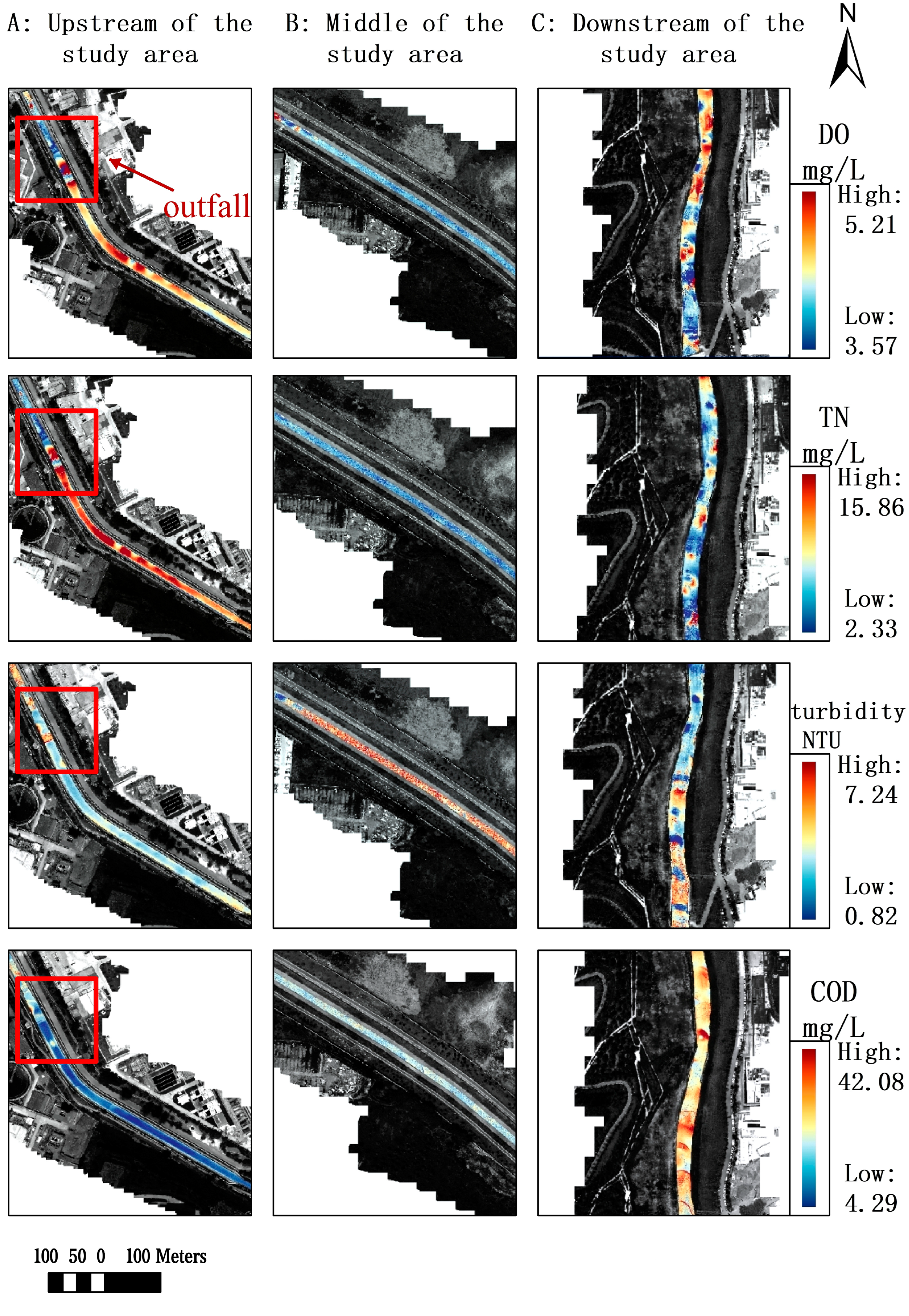
3.3. Retrieval of Water Quality Parameters

Using the optimal models for each of the four water quality parameters, the spatial distribution of water quality in the study area is depicted in Figure 6. The spatial distribution map of water quality shows that the inversion results for the DO parameter concentration ranges between 3.57 mg/L and 5.21 mg/L, between 2.33 mg/L and 15.86 mg/L for the TN parameter concentration range, between 0.82 mg/L and 7.24 mg/L for the turbidity parameter concentration ranges, and between 4.29 mg/L and 42.08 mg/L for the COD parameter concentration ranges. These results are consistent with their corresponding measured values (Figure 3 or Table 4).

From their spatial distribution, it can be observed that TN and turbidity concentrations are higher in the upstream area of the water body. Points 5 to 10 are located near sewage discharge outlets, where TN and COD concentrations increase significantly. This is believed to be due to high levels of human activity in this area, including parks, factory zones, and multiple sewage discharge outlets, which exacerbate water pollution. The concentrations of the four water quality parameters in the middle region are relatively stable. Combined with the on-site conditions of the water body, this is mainly attributed to the narrow and long stretch of the studied river segment, which does not have sewage outlets. Additionally, it is regularly managed by park authorities, and there is less vegetation coverage on both sides of this river segment. In the downstream area, the COD concentration is higher compared to the upstream and middle regions, reaching up to 42.1 mg/L. Upon an investigation and analysis of the on-site water conditions, it was found that dense vegetation growth along both banks of the water body and the influence of sediment and plants near the shore contribute to a reduced water flow velocity. This reduction in flow velocity is the primary reason for the accumulation of pollutants and the deterioration of water quality. Additionally, there are some high volumes of dissolved oxygen (DO) in both the upstream and downstream areas. This is likely attributed to the month in which sampling took place—May. This was during the summer when conditions are primarily influenced by temperature, the main factor affecting the DO content in water.

From the overall inversion results, it can be observed that the concentration of TN in this study area of the Zao River significantly increases near upstream sewage outlets. The concentrations of DO and turbidity remain relatively stable. The concentration of turbidity is higher in the midstream. However, the concentration of COD is lower in the upstream and midstream areas but higher in the downstream area, showing a gradual increase from upstream to downstream.

In previous studies, the water quality of the Zao River was very poor, with average concentrations of TN at 25.22 mg/L and COD at 137.96 mg/L across 17 monitoring sections, both exceeding “Surface Water Environmental Quality Standard GB3838-2002”, corresponding to Class V water quality [42]. Combined with Table 3, it can be observed that the water environment of the Zao River was improved. Research indicates a gradual increase in COD concentration from upstream to downstream (Dong et al., 2017) [42], which is consistent with the findings in our study.

4. Conclusions

RFE, a mainstream algorithm known for effectively selecting optimal feature subsets, is utilized in this study despite its high computational complexity. This research employs multispectral UAV technology to construct a potential feature set aimed at identifying specific water quality parameters (DO, TN, turbidity, COD). The Relief F-RFE analysis method is then employed for feature selection. Subsequently, inversion models are established for these four water quality parameters in the Zao River Basin using three machine learning algorithms (RF, SVR, LightGBM). The accuracy of the models built using different algorithms is compared, and the spatial distribution of the concentrations of the four water quality parameters is analyzed across the study area. Our main conclusions are as follows:

(1)

UAV multispectral remote sensing technology proves effective for urban river water quality inversions, as demonstrated by our models’ ability to accurately quantify the spatial distribution of four key water quality parameters in the Zao River in Xi’an. Notably, logarithmic indices emerge as pivotal features in DO parameter analysis, while combined bands are more significant in TN and COD parameter inversions. Additionally, red-edged bands dominate in turbidity parameter inversions.

(2)

Feature selection serves to eliminate redundant features. From our comprehensive accuracy evaluation results, it can be observed that the Relief F-RFE method effectively improves the models’ classification accuracy. Furthermore, integrating the Relief F-RFE feature selection method into the models enhances their fitting performance even further. The SVR algorithm that uses the Relief F-RFE method exhibits generally higher accuracy in parameter inversion. This approach offers distinct advantages in feature selection for modeling, showcasing enhanced robustness and applicability.

(3)

The spatial distribution of these water quality parameters in the Zao River study area reveals notable trends: TN concentrations increase notably near upstream outfalls, while DO and turbidity concentrations exhibit steady changes from upstream to downstream. Additionally, COD concentrations gradually rise along the river’s course, from upstream to downstream.

The Relief F-RFE feature selection optimization method adopted in this paper notably enhanced the accuracy and stability of the model. The optimization strategy employed in this model holds promise for its further applicability in experiments in other urban watersheds or lakes. The conclusions of this study may inspire residents of riverside communities to become more aware of and engaged in protecting water resources. Additionally, the inversion of water quality elements using UAV-obtained multispectral imagery is still in its exploratory phase. Given the complexity of inland rivers, it is crucial to consider additional factors such as meteorological, hydrological, and anthropogenic influences when modeling water quality parameters. Furthermore, the concept of model optimization will be refined in future work to ensure that our inversion results align more closely with the actual conditions observed.

References

1. Hoekstra, A.Y.; Buurman, J.; van Ginkel, K.C.H. Urban water security: A review. Environ. Res. Lett. 2018, 13, 53002. [Google Scholar] [CrossRef]
2. Zhao, Z.; Cao, Y.; Fan, Y.; Yang, H.; Feng, X.; Li, L.; Zhang, H.; Xing, L.; Zhao, M. Ladderane records over the last century in the East China sea: Proxies for anammox and eutrophication changes. Water Res. 2019, 156, 297–304. [Google Scholar] [CrossRef] [PubMed]
3. Basu, N.B.; Van Meter, K.J.; Byrnes, D.K.; Van Cappellen, P.; Brouwer, R.; Jacobsen, B.H.; Jarsjö, J.; Rudolph, D.L.; Cunha, M.C.; Nelson, N.; et al. Managing nitrogen legacies to accelerate water quality improvement. Nat. Geosci. 2022, 15, 97–105. [Google Scholar] [CrossRef]
4. Zhang, M.; Wang, L.; Mu, C.; Huang, X. Water quality change and pollution source accounting of Licun River under long-term governance. Sci. Rep. 2022, 12, 2779. [Google Scholar] [CrossRef]
5. Zhao, S. Inversion of Water Quality Parameters of Fuyang River in Handan City Based on Multi-Source Remote Sensing Data. Master’s Thesis, Hebei University of Engineering, Handan, China, 2021. [Google Scholar]
6. Palmer, S.C.J.; Kutser, T.; Hunter, P.D. Remote sensing of inland waters: Challenges, progress and future directions. Remote Sens. Environ. 2015, 157, 1–8. [Google Scholar] [CrossRef]
7. Feng, L.; Dai, Y.; Hou, X.; Xu, Y.; Liu, J.; Zheng, C. Concerns about phytoplankton bloom trends in global lakes. Nature 2021, 590, E35. [Google Scholar] [CrossRef]
8. Zhang, Y.; Zhou, L.; Zhou, Y.; Zhang, L.; Yao, X.; Shi, K.; Jeppesen, E.; Yu, Q.; Zhu, W. Chromophoric dissolved organic matter in inland waters: Present knowledge and future challenges. Sci. Total Environ. 2021, 759, 143550. [Google Scholar] [CrossRef]
9. Park, J.; Kim, K.T.; Lee, W.H. Recent Advances in Information and Communications Technology (ICT) and Sensor Technology for Monitoring Water Quality. Water 2020, 12, 510. [Google Scholar] [CrossRef]
10. Mamun, M.; Ferdous, J.; An, K. Empirical Estimation of Nutrient, Organic Matter and Algal Chlorophyll in a Drinking Water Reservoir Using Landsat 5 TM Data. Remote Sens. 2021, 13, 2256. [Google Scholar] [CrossRef]
11. Shi, J.; Shen, Q.; Yao, Y.; Li, J.; Chen, F.; Wang, R.; Xu, W.; Gao, Z.; Wang, L.; Zhou, Y. Estimation of Chlorophyll-a Concentrations in Small Water Bodies: Comparison of Fused Gaofen-6 and Sentinel-2 Sensors. Remote Sens. 2022, 14, 229. [Google Scholar] [CrossRef]
12. Cao, Z.; Ma, R.; Duan, H.; Pahlevan, N.; Melack, J.; Shen, M.; Xue, K. A machine learning approach to estimate chlorophyll-a from Landsat-8 measurements in inland lakes. Remote Sens. Environ. 2020, 248, 111974. [Google Scholar] [CrossRef]
13. Moses, W.J.; Gitelson, A.A.; Berdnikov, S.; Povazhnyy, V. Satellite Estimation of Chlorophyll-a Concentration Using the Red and NIR Bands of MERIS—The Azov Sea Case Study. IEEE Geosci. Remote Sens. Lett. 2009, 6, 845–849. [Google Scholar] [CrossRef]
14. Hu, Z.T.; Zhou, Y. Research on Urban Water Quality Monitoring Method Based on Low Altitude Multispectral Remote Sensing. Geospat. Inf. 2020, 18, 4–8. [Google Scholar] [CrossRef]
15. Zhu, X.; Liu, L.M.; Ye, Z.L. Unmanned aerial vehicle water quality remote sensing monitoring method. China Water Transp. 2021, 157–159. [Google Scholar] [CrossRef]
16. McEliece, R.; Hinz, S.; Guarini, J.M.; Coston-Guarini, J. Evaluation of Nearshore and Offshore Water Quality Assessment Using UAV Multispectral Imagery. Remote Sens. 2020, 12, 2258. [Google Scholar] [CrossRef]
17. Guo, Y.; Fu, Y.; Hao, F.; Zhang, X.; Wu, W.; Jin, X.; Bryant, C.R.; Senthilnath, J. Integrated phenology and climate in rice yields prediction using machine learning methods. Ecol. Indic. 2021, 120, 106935. [Google Scholar] [CrossRef]
18. Pahlevan, N.; Smith, B.; Schalles, J.; Binding, C.; Cao, Z.; Ma, R.; Alikas, K.; Kangro, K.; Gurlin, D.; Nguyen, H.; et al. Seamless retrievals of chlorophyll-a from Sentinel-2 (MSI) and Sentinel-3 (OLCI) in inland and coastal waters: A machine-learning approach. Remote Sens. Environ. 2020, 240, 111604. [Google Scholar] [CrossRef]
19. Ma, Y.; Song, K.; Wen, Z.; Liu, G.; Shang, Y.; Lyu, L.; Du, J.; Yang, Q.; Li, S.; Tao, H.; et al. Remote Sensing of Turbidity for Lakes in Northeast China Using Sentinel-2 Images with Machine Learning Algorithms. IEEE J. Sel. Top. Appl. Earth Obs. Remote Sens. 2021, 14, 9132–9146. [Google Scholar] [CrossRef]
20. Fang, X.R.; Wen, Z.F.; Chen, J.L.; Wu, S.J.; Huang, Y.Y.; Ma, M.H. Remote sensing estimation of suspended sediment concentration based on Random Forest Regression Model. J. Remote Sens. 2019, 23, 756–772. [Google Scholar] [CrossRef]
21. Yan, D.D.; Huang, Y.; Wang, D.M.; Chen, Q.W.; Wang, Z.Y.; Liu, D.S.; Zhu, Q.H.; Wei, L.L.; Hong, Y.M. Estimation of total nitrogen and total organic carbon based on UV fluorescence water quality sensor and machine learning. Acta Sci. Circumstantiae 2023, 43, 155–165. [Google Scholar] [CrossRef]
22. Xiang, X.J.; Zhang, Y.Z.; Xu, H.H.; Li, Y.; Wang, S.Q.; Zheng, Y.P. Research on Water Quality Prediction Based on CEEMDAN-VMD-TCN-LightGBM Model. China Rural. Water Hydropower. 2023. Available online: https://link.cnki.net/urlid/42.1419.TV.20231113.1049.006 (accessed on 12 March 2024).
23. Yan, Y.; Wang, Y.; Yu, C.; Zhang, Z. Multispectral Remote Sensing for Estimating Water Quality Parameters: A Comparative Study of Inversion Methods Using Unmanned Aerial Vehicles (UAVs). Sustainability 2023, 15, 10298. [Google Scholar] [CrossRef]
24. Lu, C.; Xu, S.H.; Zhu, J. Building extraction from high resolution remote sensing image based on improved U-Net model. Sci. Surv. Mapp. 2021, 46, 140–146. [Google Scholar]
25. Sankararao, A.U.; Rajalakshmi, P.; Kaliamoorthy, S.; Choudhary, S. Water Stress Detection in Pearl Millet Canopy with Selected Wavebands using UAV Based. In Proceedings of the 2022 IEEE Sensors Applications Symposium (SAS), Sundsvall, Sweden, 1–3 August 2022; pp. 1–6. [Google Scholar]
26. Zhang, C.Y.; Qiu, X.Y.; Qian, H.Y.; Liu, Y.; Zhu, J.C. Research on fault diagnosis method of turbocharger rotor based on Hu-SVM-RFE. J. Mech. 2023, 39, 344–351. [Google Scholar] [CrossRef]
27. Chen, Q.; Meng, Z.; Liu, X.; Jin, Q.; Su, R. Decision Variants for the Automatic Determination of Optimal Feature Subset in RF-RFE. Genes 2018, 9, 301. [Google Scholar] [CrossRef]
28. Jiang, X.; Zhang, Y.; Li, Y.; Zhang, B. Forecast and analysis of aircraft passenger satisfaction based on RF-RFE-LR model. Sci. Rep. 2022, 12, 11174. [Google Scholar] [CrossRef] [PubMed]
29. Marwa, H.; Bechikh, S.; Cheng, H.C. A Multi-objective hybrid filter-wrapper evolutionary approach for feature selection. Memetic Comput. 2019, 11, 193. [Google Scholar] [CrossRef]
30. Xiang, S.Y.; Xu, Z.H.; Zhang, Y.W.; Zhang, Q.; Zhou, X.; Yu, H.; Li, B.; Li, Y.F. Construction and Application of Relief F-RFE Feature Selection Algorithm for Hyperspectral Image Classification. Spectrosc. Spectr. Anal. 2022, 42, 3283–3290. [Google Scholar]
31. Mooralitharan, S.; Mohd Hanafiah, Z.; Abd Manan, T.S.B.; Muhammad-Sukki, F.; Wan-Mohtar, W.A.A.Q.I.; Wan Mohtar, W.H.M. Vital Conditions to Remove Pollutants from Synthetic Wastewater Using Malaysian Ganoderma lucidum. Sustainability 2023, 15, 3819. [Google Scholar] [CrossRef]
32. Shaanxi Provincial Local Chronicles Compilation Committee. Shaanxi Provincial Annals; Shaanxi People’s Publishing House: Xi’an, China, 1999; Volume 14. [Google Scholar]
33. Water Resources Department of Shaanxi Province. Shaanxi Provincial Water Resources Planning; Water Resources Department of Shaanxi Province: Xi’an, China, 2010. [Google Scholar]
34. HJ494-2009; Technical Specifications for Water Quality Sampling. Ministry of Environmental Protection: Shenyang, China, 2009.
35. Liang, X.L.; Pan, Z.Q.; Wang, A.P.; Yao, X.X.; Liu, L.J.; Zhou, T. Determination of Dissolved Oxygen in Water by Iodo metric method. Meas. By Chem. Anal. 2008, 17, 54–56. [Google Scholar]
36. Baulch, H.M. Asking the Right Questions about Nutrient Control in Aquatic Ecosystems. Environ. Sci. Technol. 2013, 47, 1188–1189. [Google Scholar] [CrossRef] [PubMed]
37. Hanafiah, Z.M.; Azmi, A.R.; Wan-Mohtar, W.A.A.Q.I.; Olivito, F.; Golemme, G.; Ilham, Z.; Jamaludin, A.A.; Razali, N.; Halim-Lim, S.A.; Wan Mohtar, W.H.M. Water Quality Assessment and Decolourisation of Contaminated Ex-Mining Lake Water Using Bioreactor Dye-Eating Fungus (BioDeF) System: A Real Case Study. Toxics 2024, 12, 60. [Google Scholar] [CrossRef]
38. Qiu, J.L.; Liu, Q.Y.; He, L. Chemical oxygen demand test standard and test method. Chem. Res. Appl. 2023, 35, 2809–2819. [Google Scholar] [CrossRef]
39. GB3838-2002; Environmental Quality Standard for Surface Water. Part 7: Implementation and Supervision of Standards. China Environmental Science Press: Beijing, China, 2002.
40. Jiang, Y.Z.; Kong, J.L.; Zhong, Y.L. The optimal method for water quality parameters retrieval of urban river based on machine learning algorithms using remote sensing images. Int. J. Remote Sens. 2023, 1–21, ahead-of-print. [Google Scholar] [CrossRef]
41. Ding, S.F.; Qi, B.J.; Tan, H.Y. An Overview on Theory and Algorithm of Support Vector Machines. J. Univ. Electron. Sci. Technol. China 2011, 40, 1–10. [Google Scholar] [CrossRef]
42. Dong, W.; Li, H.E.; Li, J.K.; Qin, Y.M.; Zhu, L. Analysis on water quality of severely polluted urban river, Zao River as an example. J. Hydroelectr. Eng. 2017, 31, 72–77. [Google Scholar]
Figure 1. Research area and distribution of sampling points.
Water 16 01029 g001
Figure 2. Photograph of UAV.
Water 16 01029 g002
Figure 3. Statistics of concentration values of water quality parameters in the upper, middle, and lower reaches of Zao River.
Water 16 01029 g003
Figure 4. Workflow for image processing, data analysis, and modeling.
Water 16 01029 g004
Figure 5. Importance ranking based on the SVR algorithm, with and without feature preference: (a,c,e,g) on the left, did not utilize the Relief F-RFE feature selection algorithm, while (b,d,f,h) on the right, utilized the Relief F-RFE feature selection algorithm.
Water 16 01029 g005
Figure 6. Spatial distribution of water quality parameters.
Water 16 01029 g006