Article

A Hybrid PIV/Optical Flow Method for Incompressible Turbulent Flows

by
Luís P. N. Mendes
1,*,
Ana M. C. Ricardo
1,
Alexandre J. M. Bernardino
2 and
Rui M. L. Ferreira
1
1
Civil Engineering Research and Innovation for Sustainability, Instituto Superior Técnico, Universidade de Lisboa, Av. Rovisco Pais, 1, 1049-001 Lisbon, Portugal
2
Instituto de Sistemas e Robótica, Instituto Superior Técnico, Universidade de Lisboa, Av. Rovisco Pais, 1, 1049-001 Lisbon, Portugal
*
Author to whom correspondence should be addressed.
Water 2024, 16(7), 1021; https://doi.org/10.3390/w16071021
Submission received: 19 February 2024 / Revised: 20 March 2024 / Accepted: 26 March 2024 / Published: 1 April 2024
(This article belongs to the Section Hydraulics and Hydrodynamics)

Abstract

:
We present novel velocimetry algorithms based on the hybridization of correlation-based Particle Image Velocimetry (PIV) and a combination of Lucas–Kanade and Liu–Shen optical flow (OpF) methods. An efficient Aparapi/OpenCL implementation of those methods is also provided in the accompanying open-source QuickLabPIV-ng tool enabled with a Graphical User Interface (GUI). Two different options of hybridization were developed and tested: OpF as a last step, after correlation-based PIV, and OpF as a substitute for sub-pixel interpolation. Hybridization increases the spatial resolution of PIV, enabling the characterization of small turbulent scales and the computation of key turbulence parameters such as the rate of dissipation of turbulent kinetic energy. The method was evaluated using both synthetic and real databases, representing flows that exhibit a variety of locally isotropic homogeneous turbulent scales. The proposed hybrid PIV-OpF results in a 3-fold increase in the PIV density for synthetic images. The analysis of power spectral density functions and auto-correlation demonstrated the impact of PIV image quality on the accuracy of the method and its ability to extend the turbulence range. We discuss the challenges posed by optical noise and tracer density in the quality of the vector map density.

1. Introduction

Particle Image Velocimetry (PIV) has become the standard for the non-intrusive assessment of kinematic quantities in industry as well as in applied and fundamental research. Planar PIV provides two or three dimensional velocity fields, the latter with a stereoscopic camera arrangement. Three-dimensional PIV, currently dominated by tomographic PIV, provides all three components of the velocity in volumes normally illuminated by expanded laser beams [1]. It is a relevant tool for environmental or ecological studies involving fluid mechanics, as well as aerospace, the automotive industry, civil engineering, hydraulics, fluid mechanics, and even medical and veterinary sciences. Example applications include pollutant dispersion, pollutant emission reduction, aerodynamics (planes, vehicles, or buildings), and turbulent flow analysis, as well as floods, or even blood flow studies of arterial blood vessels.
PIV methods typically assume that the region of interest is divided into small areas or volumes (interrogation areas/units—IAs), where the flow is approximately uniform. The motion of a set of particles in the interrogation units is then converted into a velocity vector through cross-correlation and sub-pixel analysis (see Figure 1). The size of the interrogation units determines the spatial resolution of PIV. Small units improve the resolution but reduce the signal quality, as the method requires several particles in the interrogation unit to obtain a strong correlation peak. Finding the correlation peak with sub-pixel accuracy is fundamental for the overall accuracy of the method. In “adaptive” or “multi-pass” PIV, this workflow is cycled several times, where, at each cycle/step, the interrogation units are refined to smaller sizes, with the number of steps/cycles being predefined by the user. The velocity vectors of each interrogation unit, from the previous step, are inherited by the newly refined units, according to a given inheritance strategy.
The resolution of classic PIV does not increase with the increase in tracer particles in the interrogation units.
Particle Tracking Velocimetry (PTV) can provide a velocity vector per tracer particle [2,3], greatly increasing the spatial resolution of classic PIV. The accuracy of Particle Tracking Velocimetry depends on the correct identification of the same particle between consecutive images and on the identification of its centroid with sub-pixel resolution. It is normally not practical for planar (2D) PIV since the out-of-plane loss of particles may reduce its advantages vis-a-vis the added computational cost. It also requires interpolation into regular grids if subsequent analysis requires evenly spaced data.
A different velocimetry technique that may provide denser 2D vector maps is optical flow (OpF). Optical flow estimates the apparent 2D flow resulting from time-varying image brightness intensity through optimization techniques. OpF methods can be classified as gradient-based, e.g., [4,5,6,7], region-based or feature-based matching [8,9,10], global-matching [11,12], spatio-temporal filtering [13,14], and, more recently, deep learning methods [15,16]. Of the many OpF methods that have been developed since their inception, most of them have specifically targeted machine vision applications; however, fluid mechanics applications started to be explored in the 1990s. The first OpF method for fluid mechanics was probably [17], featuring a global OpF method and a dynamic programming class algorithm. Other attempts at bringing OpF to the hydraulics and fluid mechanics fields are based on the Horn and Schunck [4] method. This is the case for [18] and several variants with different computational constraints [19,20,21,22]. A few other modern methods developed for fluid mechanics applications include FOLKI [23,24], Liu–Shen physics-based OpF [25], and wOFV [26,27]. Theoretically, dense OpF methods can achieve one vector per image pixel. However, the relatively sparse (identifiable) bright dots of PIV images may not allow for such high resolution.
Hybridization is a way to take advantage of favorable image characteristics, such as higher tracer concentrations, or hardware availability, such as several visualization angles by several synchronized cameras, to increase spatial resolution. Few attempts have been made at hybridizing PIV with OpF techniques. The most relevant ones include [28], with the proposal of a combination of PIV with the OpF method of Liu and Shen [25], the latter without employing any of the traditional PIV sub-pixel methods. Glomb and Swirniak (2019) [29] presented methods for hybrid PIV-OpF, as well as hybrid Particle Tracking Velocimetry (PTV), based on PIV and multi-resolution/pyramidal OpF. Seong (2019) [30] conceived a hybrid PIV-OpF approach with a Horn–Schunck-inspired method [31] that was adapted to deal with variations in laser intensity for pulsed laser configurations. The works [32,33] also developed a hybrid PIV-OpF solution that addresses image intensity variations between successive frames. It uses PIV in connection with Liu–Shen OpF [25] and with Horn–Schunck [4] OpF, where the latter provides the initial estimate for the former method. Hybrid methods have the ability to deal with large tracer particle displacements while retrieving dense velocity maps like dense OpF methods. Some hybrid PIV solutions do not require multi-resolution/pyramidal OpF setups to deal with the large displacements, for example, [28]. The novel hybrid PIV method in [34] explores a different approach to computing the cross-correlation by considering a circulant matrix and also includes a novel OpF method inspired by the Horn–Schunck formulation that better handles large displacements and that dynamically adjusts its parameters.
In summary, previous PIV-OpF hybridization efforts have attempted to streamline procedures, provide efficient implementations, test novel combinations of methods, or even present novel methods. However, there are many possible hybrid combinations of correlation-based PIV and OpF methods, mostly because there are several available OpF methods. Recently, the study [35] extensively analyzed various combinations of OpF methods and showed that the combination of the Lucas–Kanade and Liu–Shen OpF methods is the most accurate. To our best knowledge, this combination has not been hybridized with PIV. The first objective of this paper is thus to present a hybrid of correlation-based PIV and a combination of Lucas–Kanade and Liu–Shen OpF methods. We present a novel open-source tool, named QuickLabPIV-ng (https://github.com/CoreRasurae/QuickLabPIV-ng, accessed on 25 March 2024), that supports hybrid PIV with a combination of the Liu–Shen and Lucas–Kanade OpF methods [35], where the latter provides the initial estimate for Liu–Shen.
The second objective of this paper is to explore the accuracy of a hybrid PIV method that replaces sub-pixel interpolation with an optical flow (OpF) step to refine the estimation of displacement within each interrogation area. This method aims to address issues related to the size and number of particle images affecting the correlation peak’s shape, which can lead to errors in displacement estimation. By integrating OpF, the process seeks to directly correct the peak location’s integer estimate, potentially circumventing the challenges associated with traditional sub-pixel reconstruction steps in PIV analysis.
Hybrid PIV-OpF methods have been validated against well-known phenomena but not rigorously tested on real turbulent flows critical for environmental studies. Recognizing the importance of denser velocity maps for analyzing turbulence [36], this paper proposes testing these methods on realistic flows resembling homogeneous isotropic turbulence. Additionally, we highlight the limitations of applying OpF to datasets designed for classic PIV and set out to validate hybrid solutions on real-life turbulent flow data with inherent optical noise, marking a significant step toward practical application.
Finally, we validate the new hybrid PIV method and the sub-pixel OpF-based alternative on synthetic and real laboratory PIV image databases. On the one hand, validation on the synthetic databases is aimed at evaluating the raw accuracy performance by validating the methods against precise ground-truth data, as generated by the PIV image generator tool [37] (please see Section 4 for further details about the image generation). On the other hand, validation on real laboratory databases is aimed at evaluating the performance of the methods with respect to turbulent macro- and micro-scale recovery.
This paper is organized as follows. It starts with a review of the proposed PIV software and techniques. It then validates these methods using synthetic images of simple flows as a baseline, assessing errors across various noise levels. The second validation phase applies the software to real experimental data of differing qualities (in terms of image noise, non static background image elements, and varying imaged particle’s sizes and concentrations), including flows around a cylinder, in a rough boundary layer, and plunging flows. The results are analyzed using auto-correlation, structure functions, power spectral density, and dissipation rates. The paper concludes with findings and recommendations for future research.

2. Software Workflow and Main Features

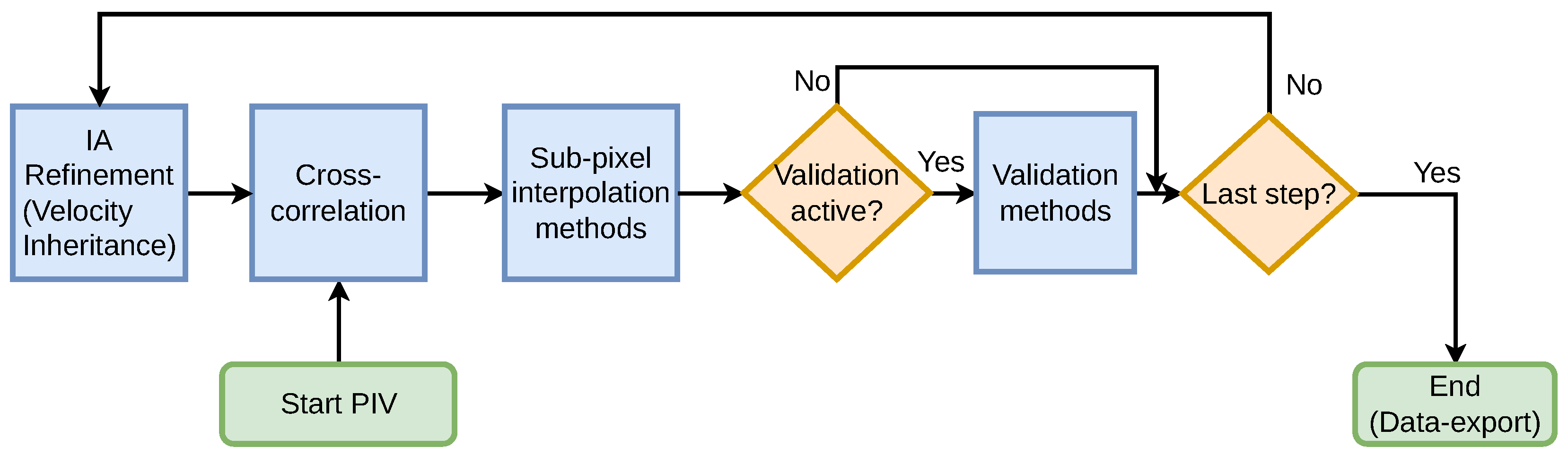
2.1. Workflow and Hybridization Options

We describe the main features and workflow of the hybrid PIV-OpF software, named QuickLabPIV-ng at version v0.8.7. The software is based on the PIV workflow. An initial coarse velocity vector field estimate is obtained by large, user-selected interrogation areas. This initial estimate is based on the cross-correlation of image pairs followed by correlation peak reconstitution to find the location of the peak with sub-pixel accuracy. The initial vector field is then inherited by smaller interrogation areas that may be deformed for better matching. Between the PIV steps, OpF may be used as a substitute for peak reconstruction and peak location. At the end of all the PIV steps, OpF may be used as the last step either to fine-tune the PIV velocity estimate or to provide denser velocity maps. Again, the number of steps/cycles is predefined by the user when selecting the starting and ending IA sizes. Between PIV/OpF steps, a vector inspection may be carried out to validate the flow field. The substitution of wrong vectors may take place. The key aspects of the workflow are depicted in Figure 2. OpF methods can be either local or global. Local OpF methods operate exclusively with an image region and vectors in the vicinity of the vector under consideration. Global OpF methods depend on the overall image to estimate any single vector and thus cannot operate with small regions.
The software supports three different hybridization variants:
  • Variant 1—“dense hybrid PIV-OpF”—employs dense optical flow as the last PIV step, either with dense Lucas–Kanade or with dense Liu–Shen combined with Lucas–Kanade. This option will provide densified velocity vector maps with 1 velocity vector per image pixel.
  • Variant 2—“sub-pixel OpF”—employs optical flow as a substitution for the cross-correlation peak reconstruction and sub-pixel interpolation to find the coordinates of the peak. This is only valid for local optical flow methods like Lucas–Kanade. It directly extracts the sub-pixel movement from the original image by considering the pixels in the vicinity of the center of each IA, thus constituting an alternative to the PIV sub-pixel.
  • Variant 3—“sparse hybrid PIV-OpF”—is similar to variant 1 but keeps only the velocity vectors of the center of each IA. We refer to this as sparse optical flow (1 velocity vector per each IA), thus keeping the original PIV vector resolution but allowing sub-pixel resolution. This supports both local and global optical flow methods, where a half-pixel warp is performed to obtain velocity pixels aligned with the center of each IA.
The process is iterated until the end of the last adaptive PIV step. Finally, the data are exported in MATLAB file format.
The following sections describe all relevant PIV and OpF methods and algorithms.

2.2. PIV Key Steps—Cross-Correlation and Sub-Pixel Interpolation

QuickLabPIV-ng features IA cross-correlation via a 2D radix-2 FFT as the main PIV method, employing adaptive multi-step processing with customizable IA window sizes. It offers various sub-pixel interpolation methods, including traditional 1D-1D Gaussian three-point polynomial interpolation [38] and 1D-1D Gaussian robust LR [39]. Additionally, it supports optical flow methods like Lucas–Kanade and its combination with Liu–Shen; see Section 2.3.

2.3. OpF Methods

The Lucas–Kanade and Liu–Shen optical flow (OpF) methods enhance fluid mechanics analysis by adapting to a wide range of imaging conditions and particle dynamics (bit depths, particle concentration, spot sizes) [35]. Lucas–Kanade, a local method, calculates displacement within a defined window, iteratively refining estimates (more details in [5]). Conversely, Liu–Shen, a global approach, improves the initial velocity estimates by incorporating physical and optical effects of image formation (e.g., light scattering and intensity), requiring a robust starting point from other methods (more details in [33]). Both techniques necessitate pre-filtering for accuracy and support adaptive iteration counts. While Lucas–Kanade quickly converges, Liu–Shen demands more iterations for refinement. However, Liu–Shen is capable of improving the accuracy over the initial velocity estimations obtained from several other methods [35]. Additionally, the software accommodates both dense and sparse applications, offering a specialized Liu–Shen mode for clipped images, allowing CPU implementation, albeit with compromised precision.

2.4. Hybridization of OpF and PIV after Correlation Steps

QuickLabPIV-ng enhances PIV analysis by enabling the use of two distinct sub-pixel interpolation methods at various stages, optimizing the initial and final interrogation steps with separate techniques. This dual approach allows for the initial use of either sparse OpF or traditional sub-pixel methods, transitioning to dense OpF methods for final refinement. This strategy not only improves sub-pixel accuracy, particularly in the last steps, but also densifies velocity maps for more detailed results. The software’s flexibility in combining OpF and traditional methods offers significant advantages in precision and computational efficiency, bypassing traditional warping methods for a direct, accurate sub-pixel resolution. While standard sub-pixel techniques determine displacement by analyzing the geometry of cross-correlation peaks, optical flow (OpF) methods directly compute fractional displacement from the raw image. When the interrogation area (IA) size in the final PIV step is smaller than the OpF window, using dense OpF becomes more cost-effective and reduces the drawbacks of global methods. An OpF approach can bypass traditional PIV warping, offering a direct transition to precise sub-pixel measurements, maintaining an accuracy comparable to that of conventional warping techniques.

2.5. Vector Inheritance and Warping

When iterating to the next PIV step, i.e., smaller IA sizes, the processing continues with the refinement of interrogation areas (IAs) into smaller areas and includes a vector inheritance strategy, as well as an IA image warping strategy. When all adaptive PIV steps are completed, PIV processing proceeds with a possible hybridization (either variant 1 or variant 3). If hybridization is to be performed, then a single pass of optical flow is applied. We refer to methods featuring image warping as “Modern PIV”.

2.5.1. Vector Inheritance

The vector inheritance strategy involves selecting a method—area, distance, or bi-cubic spline interpolation—to import velocity vectors before adjusting the second image’s interrogation area (IA) windows accordingly for cross-correlation. Each method offers a unique way to calculate new IA displacements based on previous steps: area inheritance uses a weighted average from overlapping IA areas (see Figure 2), distance inheritance applies weights inversely proportional to the center distances of adjacent IAs, and bi-cubic spline inheritance interpolates displacements using a 2D map of IA centers. The Bi-cubic spline is noted for its superior accuracy in validations with synthetic image databases (see Section 3).

2.5.2. IA Image Warping

Window warping PIV employs backward image warping or a blend of window displacement and image warping, rather than shifting interrogation areas (IAs) by inherited displacements. This approach includes full or partial warping methods—traditional warping, mini-warping, and micro-warping. Traditional warping applies bi-cubic spline-interpolated displacements to each pixel, ensuring no voids or overlaps and maintaining fixed IA window locations. Mini-warping and micro-warping adjust IA windows based on estimated displacements, with micro-warping focusing on integer displacements followed by fractional warping for precision. QuickLabPIV-ng supports various configurations for applying warping to enhance PIV accuracy, with micro-warping on the second image showing the best results in validations; see Section 3.

2.6. Vector Validation and Substitution

Vector validation in PIV systems identifies and addresses incorrect velocity vectors caused by a low SNR, insufficient correlatable data, or other issues like boundary effects and particle movement. QuickLabPIV-ng offers methods to mark invalid vectors as zero or “not a number” for data export and to correct for such vectors where feasible, using a combination of validation and vector replacement techniques. These techniques ensure the reliability of the velocity data by effectively identifying and addressing outliers.
QuickLabPIV-ng implements two primary methods for vector validation: difference validation and normalized median validation [38]. The first evaluates the differences in the velocity vector within a local grid, flagging those that exceed a set threshold as invalid. The latter uses a median-based approach, comparing each vector with the median vector within its vicinity against a normalized threshold to determine validity.
| | u m e d u ( i , j ) | | r m e d + ϵ 0 θ t h r e s h o l d ,
where u m e d denotes the vector with the median Euclidean norm of all the vectors in the neighbor IAs; u ( i , j ) is the vector under analysis; r m e d is the median of the residuals r i = | | u i u m e d | | , where i = 1 ,   ,   8 indexes the neighbor IAs; and ϵ 0 is a regularization term between 0.1 and 0.2 pixels.
QuickLabPIV-ng offers two methods for vector replacement: bi-linear and multi-peak. Bi-linear interpolation generates a new vector from valid neighboring vectors, while multi-peak searches for alternative high-correlation peaks as potential replacements, assuming the primary peak might be noise-distorted. If multi-peak fails, it defaults to bi-linear interpolation. The software also supports iterative validation to refine vector accuracy, though with caution to avoid misjudging valid vectors as invalid. This process enhances data reliability, especially in low-signal-to-noise scenarios.

3. Verification and Validation of the Hybrid PIV-OpF Software

3.1. Strategy

In this section, we evaluate the performance of QuickLabPIV-ng PIV on synthetic and real datasets according to the three variants described in the previous section. The evaluation of synthetic data performance focuses on accuracy and spatial error distribution compared to the ground truth across synthetically generated datasets. The evaluation uses a PIV image generator tool [37], enhanced in version 1.2.0 to differentiate between wall and flow regions [40], exemplified in [35] in a Poiseuille flow scenario. The methodology includes analyzing a Statistical Image Group (SIG) comprising images with varying parameters like flow type, maximum velocity, bit depth, white noise variance, and particle size and concentration. The evaluation calculates both average relative and absolute errors across the entire SIG, excluding vectors with no ground-truth velocity. Additionally, it assesses in-plane ( F i ) and out-of-plane ( F o ) particle losses for PIV methods. For hybrid PIV methods, in-plane losses cannot be measured due to the absence of interrogation areas in the final step, and out-of-plane losses are estimated using the standard deviation of movement. Although the study tested various bit depths, the discussion focuses on 8-bit results due to their similarity.
For real experimental data, the analysis focuses on power spectral density, structure functions, and auto-correlation functions using laboratory PIV data. This qualitative assessment aims to determine whether hybrid PIV, utilizing either the Lucas–Kanade method alone or in combination with the Liu–Shen method, enhances the effective measurement range over standard PIV methods. This includes evaluating improvements in capturing the auto-correlation, power spectral density, and 2nd -order structure function of velocity fluctuations. Hybrid PIV’s ability to analyze down to individual pixels could potentially expand the data range from regular PIV datasets, especially in turbulent flows and across varying image qualities.

3.2. Synthetic Data

3.2.1. Comparison of Correlation-Based PIV Implemented in QuickLabPIV-ng with State-of-the-Art PIV

We tested five flow types, namely, uniform flow, inviscid flow with a stagnation point, Rankine vortex, Rankine vortex with superimposed uniform flow, and planar Poiseuille flow. All flows were generated for each combination of particle spot diameter ( 1.0 , 2.0 , 3.0 , and 6.0 pixel spot sizes); White Gaussian Image Noise (WGIN) ( 0.0 , 5.0 , and 15.0 dB); maximum velocity displacement vector ( 0.8 , 1.6 , and 4.0 px/frame); particle concentration per IA volume (1, 6, 12, and 16 particles/IA volume); and standard out-of-plane movement ( 0.025 , 0.050 , and 0.100 mm).
The traditional PIV of QuickLabPIV-ng’s modern PIV approach was evaluated against the state-of-the-art OpenPIV, at version 0.25.0. OpenPIV applies warping to each IA pair, followed by a cross-correlation of each warped IA pair and ending with a sub-pixel method. OpenPIV also includes a bi-cubic spline based velocity filter/smoothness method and integrates vector validation techniques.
Figure 3 provides an overview of the relative accuracy for the traditional PIV mode between QuickLabPIV-ng and OpenPIV. As we can see, considering the median, QuickLabPIV-ng is within 3 dB of OpenPIV, with the latter having a slight general advantage.

3.2.2. Accuracy of QuickLabPIV-ng by Flow Type

In this sub-section, we analyze several performance aspects, accuracy-wise, with respect to the synthetic image databases. We start with an assessment of the relative performance between warping PIV in QuickLabPIV-ng with respect to the well-known and state-of-the-art OpenPIV with regard to the non-hybrid PIV modes; see Figure 3. It is not our intent to benchmark this tool against OpenPIV, or other any other PIV tool; we just want to show that QuickLabPIV-ng’s base PIV with warping is mostly in line with OpenPIV’s performance.
Figure 4 evidences the accuracy advantage of employing a final step of sparse OpF with Liu–Shen combined with Lucas–Kanade, for all the considered flows, with respect to the standard sub-pixel employed in standard PIV with warping.
In Figure 5, it can be seen that hybrid PIV slightly improves the advantage observed for the OpF sub-pixel in standard PIV (compared with Figure 4) for all the flows. The Poiseuille flow has a more pronounced advantage for hybrid PIV, which is due to the smaller proportion of highly erroneous vectors to the total number of velocity vectors.

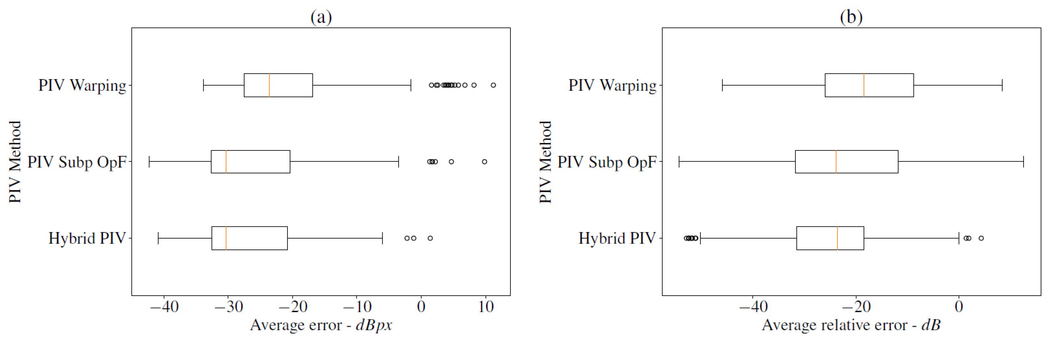
3.2.3. Overall (All Flows) Accuracy Span

Figure 6 depicts the results averaged across all the flow types for the three methods—PIV with warping, PIV with warping combined with a final OpF sub-pixel, and hybrid PIV. The OpF sub-pixel improves the accuracy but also increases the variance in the relative error, particularly for the smallest particle spot sizes. The introduction of hybrid PIV techniques yields dense data with comparable accuracy to PIV enhanced by the OpF sub-pixel while also reducing the variance observed in relative errors. This indicates a balance between improved detail and the stability of measurement outcomes.
Figure 7 summarizes the absolute error versus effective particle concentration per IA volume with respect to different particle sizes and WGIN noise levels. A PIV method with micro-warping (left) and two hybrid PIV methods, one with Lucas–Kanade OpF (middle) and another with Liu–Shen combined with Lucas–Kanade OpF (right), are evaluated. The relative errors are not shown since the performance is similar for this flow. Figure 8 rearranges the data to compare relative errors against particle spot sizes and flow types with a constant displacement of 4.0 px/frame. It assesses the average relative error across various WGIN noise levels for the three PIV methodologies: a PIV method with micro-warping (left) and two hybrid PIV methods, one with Lucas–Kanade OpF (middle) and another with Liu–Shen combined with Lucas–Kanade OpF (right). The absolute errors are not shown since the performance is similar.
The findings in Figure 7 and Figure 8 suggest avoiding 1.0 px particle sizes across all methods and generally steering clear of low concentrations, like 1 particle per IA, except possibly in hybrid PIV with larger particles and minimal noise. The Poiseuille flow posed the greatest challenge, unlike the more straightforward uniform flow. Accuracy did not significantly vary with particle sizes of 3.0 px and above or concentrations over 6 particles per IA in OpF methods. The optimal results were seen with 16 particles per IA and 3.0 px sizes, though larger 6.0 px particles showed reduced variance, not necessarily improving accuracy.

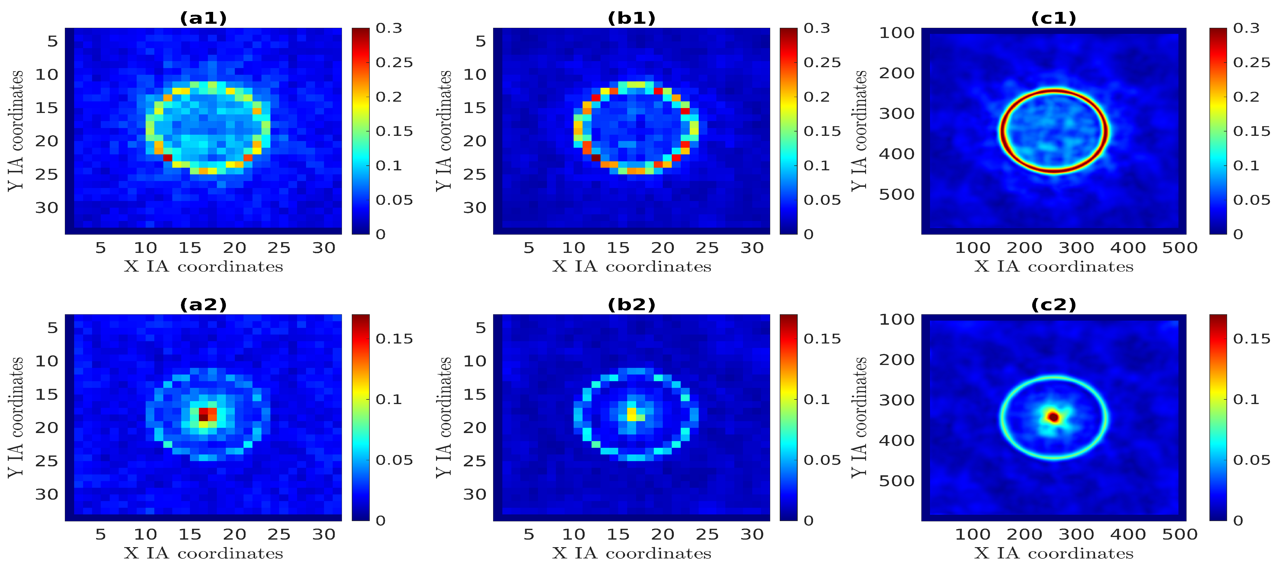
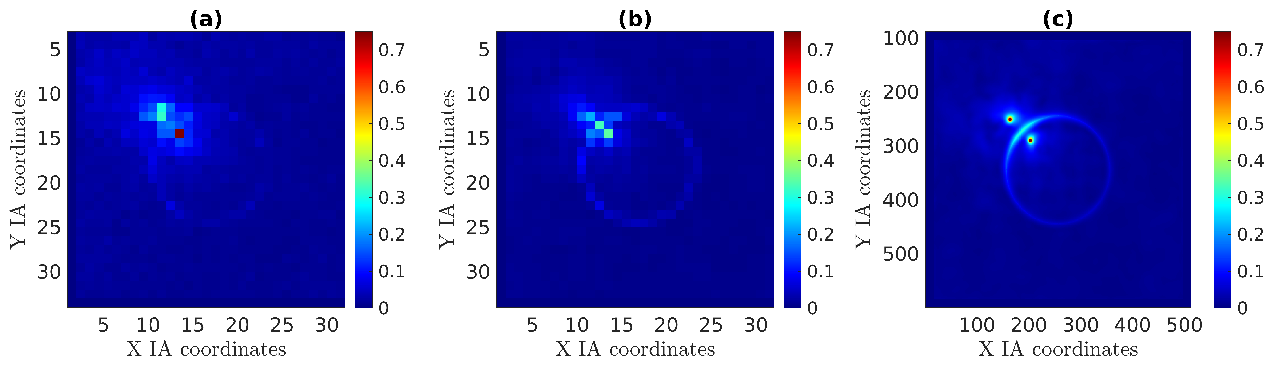
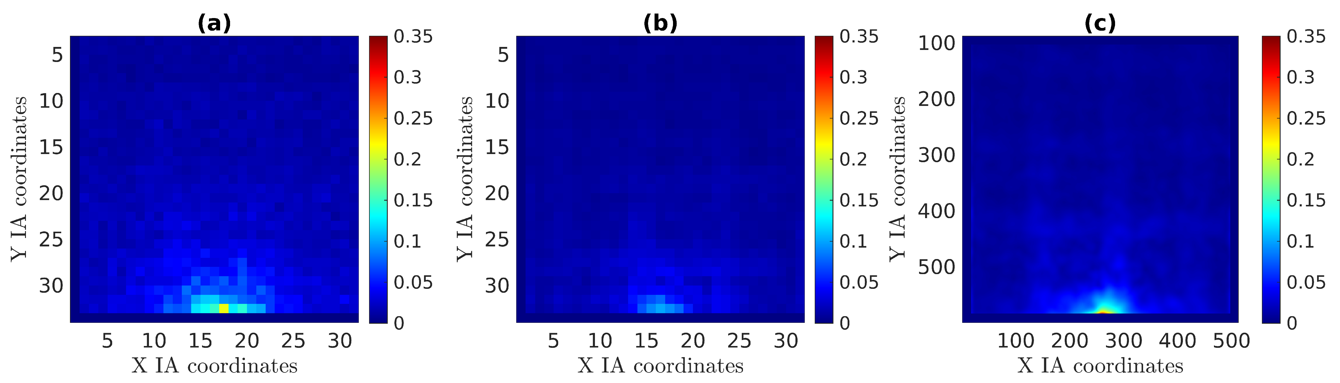
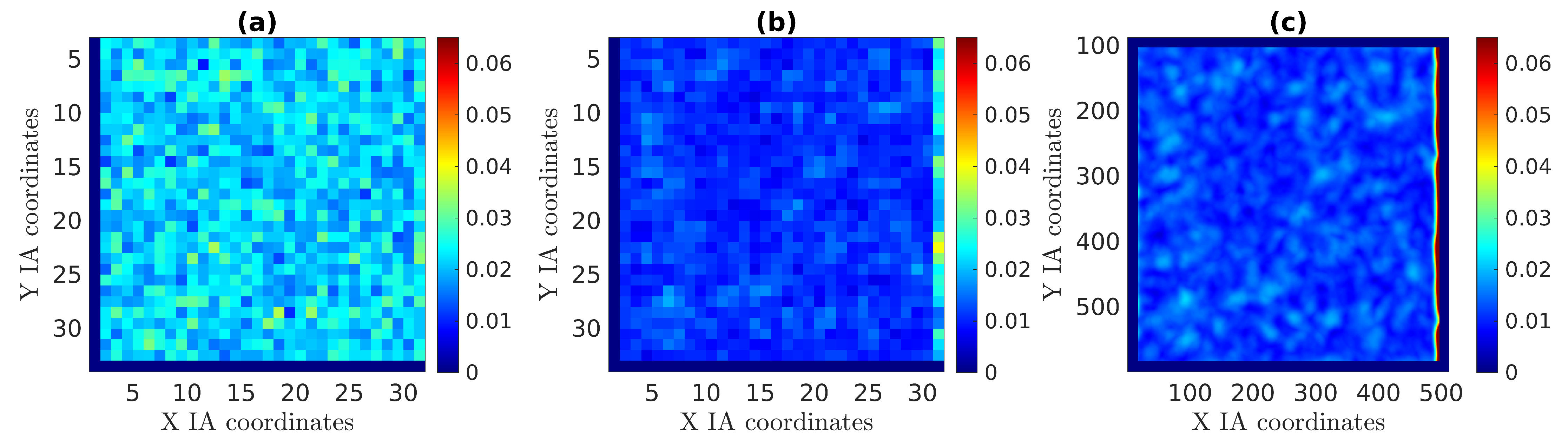
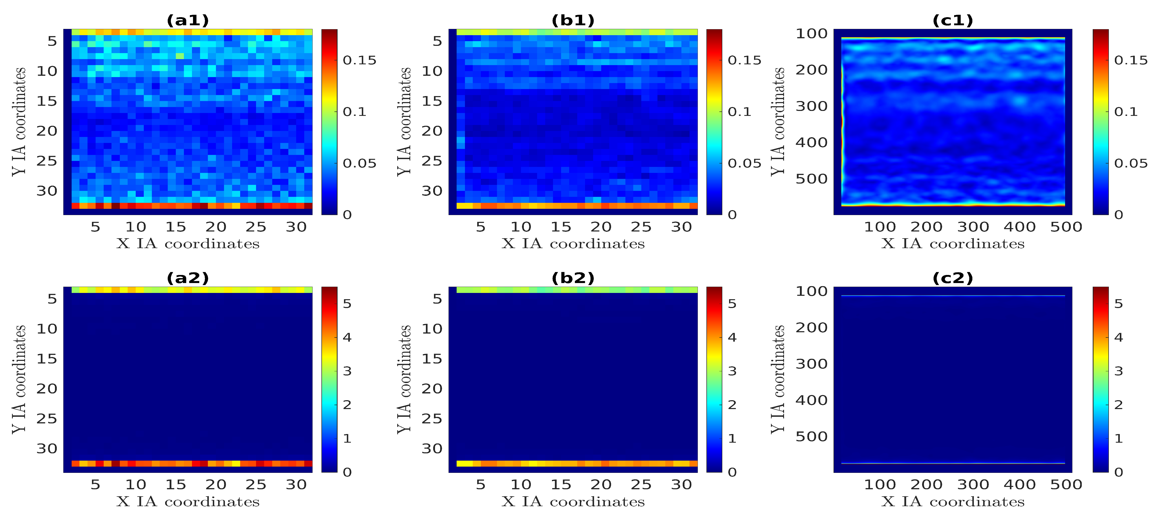
3.2.4. Spatial Error Distribution

This study examines the spatial distribution of absolute and relative errors across various flow types: Poiseuille, Rankine vortex, Rankine vortex combined with uniform flow, inviscid flow with a stagnation point and uniform flow. All flows have 3.0 px diameter particles with a concentration of 12 particles per IA, a maximum velocity of 4.0 px/frame, and a WGIN noise level of 0 dBW. The evaluation encompasses three methods: micro-warping PIV; micro-warping PIV enhanced with a sparse sub-pixel approach based on Liu–Shen combined with Lucas–Kanade OpF in the final step; and dense hybrid PIV utilizing Liu–Shen with Lucas–Kanade OpF. These methods, which do not include vector validation, were assessed using adaptive PIV strategies, specific pixel width settings for the sub-pixel analysis, and distinct iterations and window sizes for the Lucas–Kanade and Liu–Shen algorithms, highlighting the performance of each configuration under the given conditions.
In the Poiseuille flow analysis (Figure 9), the highest inaccuracies were noted near the horizontal walls at the top and bottom. The micro-warping PIV method exhibited the largest average error in both relative and absolute terms, surpassed by the sparse OpF sub-pixel PIV in error magnitude. The hybrid PIV method demonstrated superior performance, showing a significantly smaller proportion of highly erroneous vectors (Table 1). Notably, the most significant errors in the hybrid PIV method were confined to narrow regions near the top and bottom, each about 1 px in width.
In Figure 10, the Rankine vortex presents two challenging areas: one involving the absolute error at the boundary between the forced and free vortex regions, and another concerning the relative error at the vortex center where the velocity is zero. Table 2 illustrates that the OpF sub-pixel enhances accuracy compared to standard warping PIV. The hybrid method, equivalent to the OpF sub-pixel, maintains the mean accuracy while offering detailed velocity maps. Hybrid Lucas–Kanade achieves similar accuracy to warping PIV but with the added benefit of denser velocity data.
The Rankine vortex combined with a uniform flow shows similar patterns of absolute errors to the Rankine vortex alone but with reduced severity due to the velocity division between the vortex and uniform flow. In terms of relative errors, two zero-velocity regions pose challenges (Figure 11). Overall, across the entire image area, the trend observed with the Rankine vortex persists, indicating that hybrid PIV maintains a comparable mean accuracy to standard PIV methods, as highlighted in Table 3.
For the inviscid flow with a stagnation point (Figure 12 and Table 4), the relative errors are low across all methods, making them less noteworthy. The distinction comes with the absolute errors, which exhibit similar patterns for both PIV and hybrid PIV to those seen in other flow types. Specifically, PIV enhanced with Liu–Shen and Lucas–Kanade OpF outperforms standard PIV, and when this combination is applied in hybrid PIV, it achieves comparable accuracy with the benefit of denser velocity maps. Similarly, hybrid PIV using dense Lucas–Kanade matches the accuracy of standard PIV, also providing denser velocity data.
With respect to the uniform flow, we see that the best results are obtained when the Liu-Shen combined with Lucas-Kanade is employed, as documented by Figure 13 and Table 5, both for PIV with OpF sub-pixel and dense hybrid PIV modes. The relative results are not shown since the error distribution is similar to the absolute errors. The uniform flow achieves the best accuracy of all the considered flows, posing the least challenge for all of the algorithms considered.

3.3. Laboratory Databases

3.3.1. Description of Databases and Validation Criteria

We employed three different PIV image databases from different experiments, all grayscale with 8-bit depth images, but with varying image quality with respect to particle spot sizes, concentrations, and background noise. A different flow type is represented by each database:
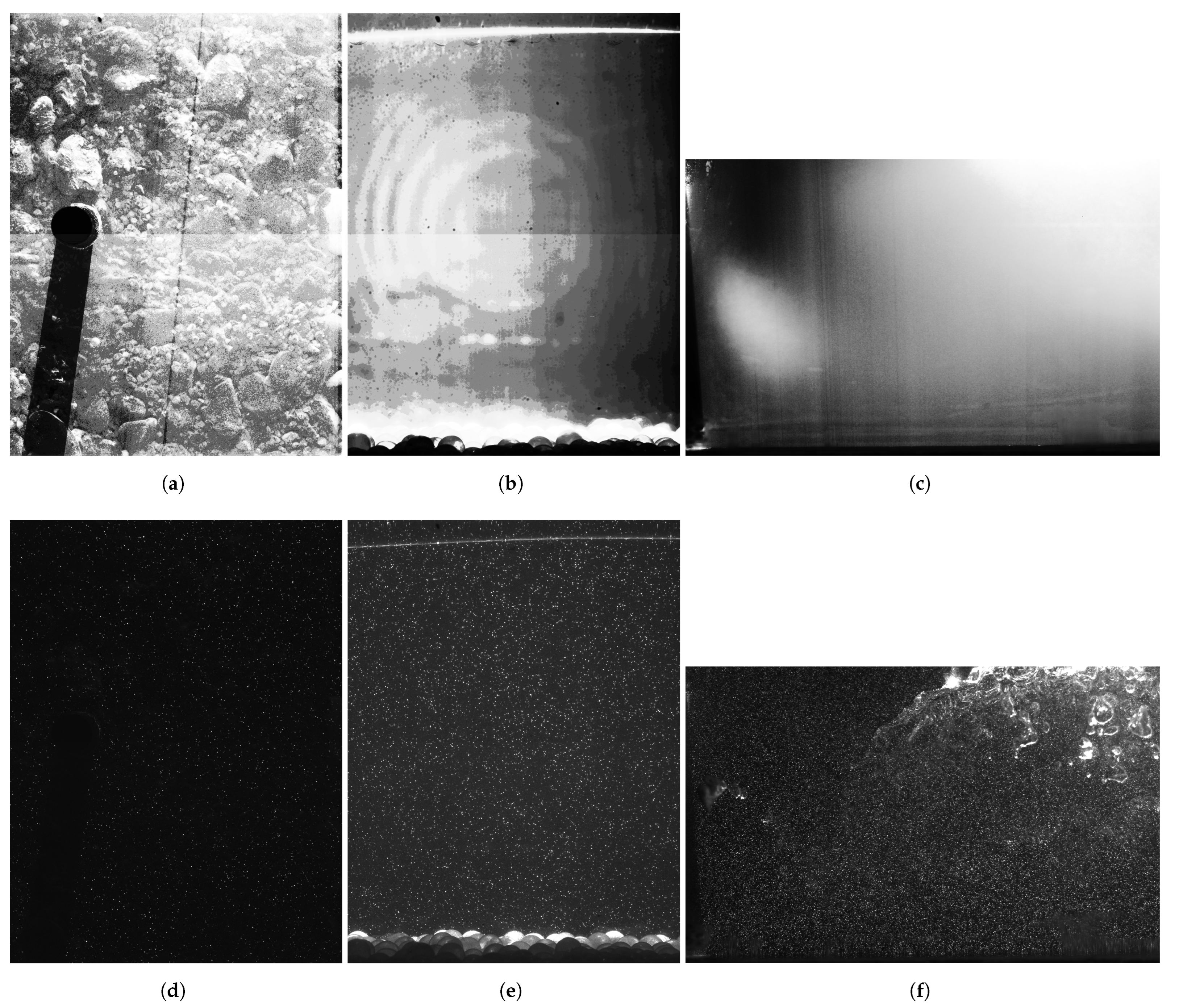
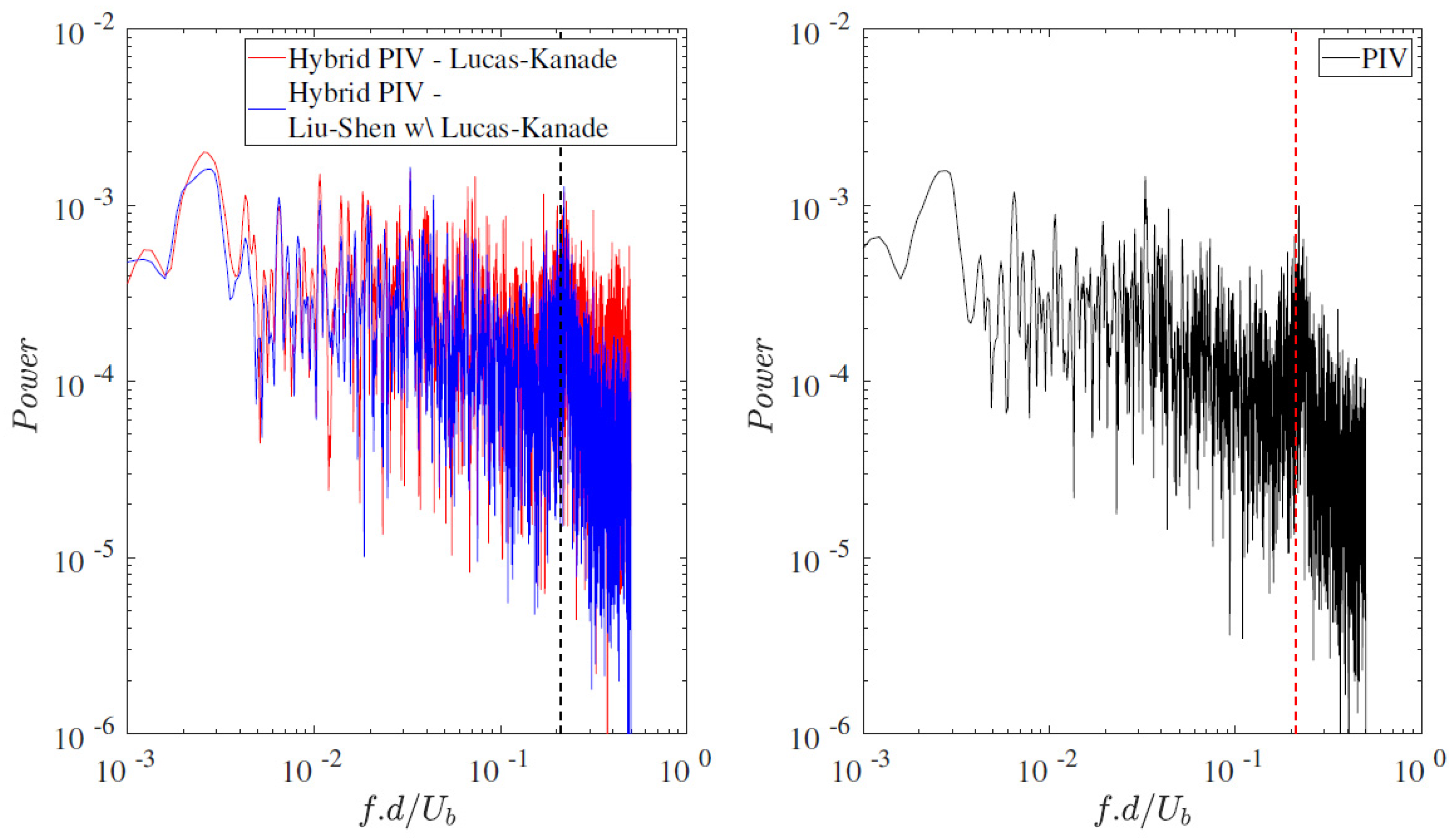
  • Cylinder database: The images were obtained from a flow around a wall-mounted smooth circular cylinder. The flow is characterized by the Reynolds number based on the cylinder diameter, R e = d U b / ν equal to 1750, where d is the cylinder diameter, U b is the approaching velocity, and ν is the kinematic viscosity. The measured plane corresponds to the horizontal plane (longitudinal-spanwise direction) located at 60 % of the flow depth. The database is composed of 4500 poor-quality PIV image pairs having a 1600 × 1200 px 2 resolution. The particle spot sizes are not within the optimal PIV range, being on the smaller side, and the particle concentration is also low. There is a background pattern in the PIV images, and there is a cable harness that oscillates during the PIV recording (Figure 14a). This is an image quality that should also prove difficult for OpF, since OpF is known to also have difficulties with average particle diameters smaller than 2.0 px. Still, we wish to compare the performance of hybrid PIV with this image database, for which we have two validations: obtain the expected peak in the energy spectrum in the cylinder’s wake and find the expected properties of undisturbed flow.
  • Boundary layer database: A database composed of 4500 fair-quality PIV image pairs with a 1600 × 1200 px 2 resolution, acquired from a turbulent open-channel flow over a glass bead fixed bed. The acquired data correspond to a vertical plane (longitudinal bed-normal direction) located at the channel center line. The images have a static background pattern, as shown in Figure 14b. The seeding quality is on the average side. This database is to be validated in accordance with the known features of boundary layer flows.
  • Plunging flow database: The images were obtained from a complex flow in a dam break flume setup. The measured plane corresponds to a vertical plane (longitudinal bed-normal direction) located in the breach region at 0.5 cm from the channel side wall. The database is composed of 1817 PIV image pairs, with a resolution of 1920 × 1200 px 2 , adequate particle spot sizes, and good image quality with a higher particle concentration than the other two databases. The images have no special background pattern (Figure 14c); however, there are two regions that tend to form large air bubbles, which can affect the measurements.
Hybrid PIV started at an IA resolution of 128 × 128 with 50 % overlap and went to 16 × 16 with 50 % overlap, employing micro-warping on the second image and applying Hongwei Guo’s robust linear regression of the 1D-1D Gaussian function as the sub-pixel method. Validation was also applied to PIV at the end of each adaptive step by employing the normalized median validation, employing secondary peak replacement up to the 4th secondary peak and having a final substitution backup with linear interpolation. Hybridization with Lucas–Kanade was performed by applying a single final step of the Lucas–Kanade OpF method, either with or without a Gaussian filter. Dense results were exported without validation applied to the final OpF step. Lucas–Kanade OpF was set up with 5 iterations and a window size of 27 px, and the Gaussian filter, when applied, had a width of 3 pixels and a standard deviation ( σ ) of 2.0 px. Hybridization with Liu–Shen combined with Lucas–Kanade followed the same base configuration as hybrid PIV with Lucas–Kanade, but with the Gaussian filter always enabled. Liu–Shen OpF was applied after the first pass with Lucas–Kanade. Liu–Shen was set up with 60 iterations, a Lagrange multiplier value of 4, and a Gaussian filter of 3 px width and a standard deviation of σ = 0.48 px. PIV with warping with the Hongwei sub-pixel at all adaptive steps was set up in exactly the same way, with the exception that the last step with OpF was disabled. Another PIV method under test was PIV with warping that employed Hongwei Guo’s sub-pixel for the initial adaptive steps and the Lucas–Kanade OpF sub-pixel for the last adaptive step, otherwise sharing the same setup with the PIV with warping. Classic PIV with Lucas–Kanade at all adaptive steps did not employ warping at all, and it had Hongwei Guo’s sub-pixel replaced by Lucas–Kanade OpF at all adaptive steps.

3.3.2. Cylinder Database

Turbulent flows around wall-mounted smooth cylinders, which have been widely studied, are characterized by alternating vortex shedding due to flow separation on the cylinder. The normalized shedding frequency, named the Strouhal number, for flows with Reynolds numbers between 1000 and 4000 is approximately constant and equal to 0.21  [41]. The Strouhal number is defined as S t = f × d / U b , where f is the frequency, d is the cylinder diameter, and U b is the approaching velocity.
Figure 15 presents the energy spectrum at a point in the wake of the cylinder, following the Taylor hypothesis. The energy peak corresponding to the shedding frequency is well identified by both PIV and the hybrid methods. The hybrid PIV method with Lucas–Kanade generates a noisier spectrum than the other methods; nevertheless, an energy peak is detectable at the expected shedding frequency.
Sufficiently outside of the cylinder influence, the theoretical condition of homogeneous and isotropic turbulence is applicable, and, thus, an inertial range of scales characterized by the 5 / 3 law is expected [42] (pp. 248–274). The inertial range of scales corresponds to scales that are not directly affected by the energy maintenance and dissipation mechanisms and where merely a transfer of energy, from production processes to dissipation processes, occurs. For that scale’s range, the energy spectrum, E ( k ) , is described by E ( k ) = c ϵ 2 / 3 k 5 / 3 , where c is a universal constant, ϵ is the rate of energy dissipation, and k is the wave number.
To assess the ability of the hybrid methods to improve the spatial resolution for the cylinder database, a longitudinal strip of data was selected on the left-hand-side end and employed to compute the power spectral density (PSD) functions depicted in Figure 16. The results for PIV methods, without an appreciable difference between methods, show, approximately, an energy spectrum with the expected 5 / 3 slope for k between 60 and 600 m 1 , despite its noisy shape. Likely due to the low quality of the images in this database, the smallest scales of the PIV methods deviate from the 5 / 3 law without any physical justification. Relative to the hybrid method’s behavior, the spectra are similar to those obtained by PIV methods until k = 300 m 1 , deviating from the 5 / 3 law for larger wave numbers. The hybrid methods with Lucas–Kanade only, with or without a Gaussian filter, show a slope smaller than 5 / 3 , while the method of Liu–Shen with Lucas–Kanade presents a faster rate of energy transfer to smaller scales. None of the methods recovers the expected 5 / 3 slope, indicating that, for this database of poor quality, the hybrid methods are not able to adequately improve the spatial resolution of the spatial data.

3.3.3. Boundary Layer Database

A turbulent open-channel flow over a rough fixed bed is characterized by the well-known boundary layer theory. To evaluate the adequacy of employing hybrid methods to extend the spatial resolution, we computed, for each tested method, the auto-correlation function and the energy spectrum of a longitudinal profile of the flow velocity sampled at 7 % of the flow depth (i.e., a line parallel to the bed at about 5 mm above the crest level). The velocity profile consists of a series of time-averaged longitudinal velocity components.
The auto-correlation presented in Figure 17 shows no appreciable difference among different PIV and hybrid methods. Moreover, for all the tested methods, the auto-correlation function is approximately zero for a space lag r = 1 cm. The main difference is observed for the smallest space lags. Hybrid PIV with dense Lucas–Kanade without a Gaussian filter and classic PIV with the Lucas–Kanade sub-pixel show larger noise levels than the other methods.
Figure 18 presents the power spectrum density (PSD) data, showing the expected 5 / 3 slope for all methods except for the hybrid PIV with Liu–Shen combined with Lucas–Kanade. Nevertheless, hybrid PIV with LK and classic PIV with LK for all steps led to better results, as the 5 / 3 slope applies to a larger range of scales. The inertial range of scales of the studied boundary layer flow is expected to span to scales on the order of a few millimeters. The PIV methods with Hongwei generate PSD functions deviating from the 5 / 3 slope close to the tail, likely due to noise effects, rendering an unexpected short inertial range of scales. The results from the hybrid methods with dense LK are encouraging, as the spectral analysis renders the extension of the inertial range of scales as expected. An increase in the noise level is visible for the smallest scales, in accordance with the observations from the auto-correlation function; however, this noise level does not compromise the main result: the identification of the inertial range of scales spanning from k = 200 m 1 to k = 5000 m 1 .
In summary, the results for images of moderately good quality indicate that the hybrid methods with dense LK can improve the spatial resolution relative to classic PIV methods. Such an improvement is of paramount importance for turbulence analysis, allowing, for example, the computation of Taylor’s micro-scale from the auto-correlation function or the dissipation rate from the energy spectrum.

3.3.4. Plunging Flow Database

In this database, all the methods have smooth and compatible auto-correlation functions (see Figure 19). With respect to the power spectral density (PSD), as shown in Figure 20, all methods present high compatibility, with the hybrid PIV methods achieving the full pixel resolution for this database. The Gaussian filter applied to the hybrid PIV Lucas–Kanade results in a power reduction for the final range of wave numbers, thus possibly reducing image noise to some extent but also potentially modifying the spectral information. Hybrid PIV with Liu–Shen combined with Lucas–Kanade again extends the PIV slope to higher wave numbers, essentially following the PIV slope with respect to the PSD.
The results from this database, composed of images of good quality, lead to the conclusion that the hybrid methods can be adequately employed to improve the spatial resolution relative to classic PIV methods.

4. Methods and Materials

We cannot provide the test databases online due to their sheer size, as we would not be able to guarantee the medium- to long-term availability of the contents. We thus prefer to provide instructions to generate similar ones for the synthetic image database. As for the experimental databases, the authors are willing to provide them upon request.
It should, however, be noted that these databases are not a critical part of the article and that their role is just to document the PIV and hybrid PIV methods’ capabilities. As such, the results presented are expected to be compatible with other results obtained from other databases with similar characteristics.
Other than that, as of this writing, the recommended version to reproduce these results is QuickLabPIV-ng v0.8.7, obtainable from https://github.com/CoreRasurae/QuickLabPIV-ng/releases/tag/v0.8.7 (accessed on 25 March 2024). The software itself does most of the computation without requiring external libraries/frameworks; namely, image filtering, cross-correlation, and Lucas–Kanade and Liu–Shen optical flow methods are implemented internally, which should protect the software from bit-rot, as well as unexpected behavioral changes coming from external library updates. Even with this effort made, it was not completely possible to avoid an important dependency on the Aparapi (https://aparapi.com (accessed on 25 March 2024), https://git.cleverthis.com/cleverthis/aparapi/aparapi/-/releases/v3.0.2 (accessed on 25 March 2024)) library/framework, which enables High-Performance Computing (HPC) for Java in systems with GPU or CPU devices supporting OpenCL.
Besides the software, it requires a computer with at least 32 to 64 GB of RAM for medium- to large-sized databases. Ideally, the system should be a multi-core computer with at least one AMD® or NVIDIA® GPU. Discrete Intel® GPUs have not been tested yet, but integrated Intel® GPUs are known to produce invalid results with the current versions of QuickLabPIV-ng/Aparapi. A Java virtual machine compatible with at least Java 8 should be employed, and it has been tested in both Windows® and Linux environments. Currently, QuickLabPIV-ng only supports image depths of 8 bits from the GUI. We ran our databases on a system with 64GB of RAM by invoking QuickLabPIV-ng with java -Xmx48G -jar QuickLabPIVng.jar.
A synthetic image database can be easily generated from piv-image-generator [37] but using the latest code from https://git.qoto.org/CoreRasurae/piv-image-generator/-/releases/v1.2.0 (accessed on 25 March 2024). All that is required is to edit the main configuration/script file ‘exampleAllTestImagesMain.m’ and adjust the following contents:
displayFlowField=false;
closeFlowField=true;
flows={′uniform′ ′parabolic′ ′stagnation′ ...;
′rankine_vortex′ ′rk_uniform′};
bitDepths=[8];
deltaXFactor=[0.05 0.10 0.25];
particleRadius=[0.5 1.0 1.5 3.0];
Ni=[1 6 12 16];
noiseLevel=[0 5 15];
outOfPlaneStdDeviation=[0.025 0.050 0.100];
numberOfRuns=10;
generatePIVImagesWithAllParametersCombinations;
All software was developed in-house and is available as open-source. The PIV hardware equipment, namely the PIV Laser lighting and image acquisition hardware, was obtained from Dantec Dynamics A/S, Skovlunde, Denmark.

5. Conclusions and Recommendations for Further Analysis

The main conclusion of this research is that hybrid PIV-OpF can improve PIV’s resolution and ability to provide data adequate to analyze fine-scale turbulence. While a better resolution of the mean flow is easy to achieve, turbulence statistics are improved only if the raw PIV images are of good quality, i.e., are within the optical range of tracer density and spot size, and have low optical noise. Hybrid PIV with Liu–Shen and Lucas–Kanade offers the highest accuracy in the description of the mean flow. However, in real databases, it may not closely follow the expected PSD slope of −5/3, despite extending the slope for higher frequencies, suggesting a potential for noise filtering.
To analyze turbulence, the Lucas–Kanade algorithm alone is preferable. It correctly reproduces the flow’s macro-scales and the slope of the power spectral density function and does so in locally isotropic homogeneous turbulence. It is also computationally more efficient.
Integrating Liu–Shen with Lucas–Kanade optical flow (OpF) as an alternative to interpolation peak reconstitution with sub-pixel accuracy is a valid alternative, especially in essentially 2D flows with high-quality images. In this case, the method achieves the accuracy of traditional PIV methods employing warping. PIV’s last adaptive step with a Lucas–Kanade OpF step maintains the standard PIV workflow while leveraging the precision benefits of optical flow techniques.
From our experience, independently of the method, the optimal image conditions include particle sizes around 3 px and at least 6 particles per IA, improving with higher concentrations. For the analysis of PIV sequences, a tailored approach is recommended for optimal results. For classic PIV incorporating optical flow (OpF) for sub-pixel refinement, the sparse Lucas–Kanade method is preferred. If initial sub-pixel interpolation deviates significantly from expectations, it is advisable to limit the OpF application to the final refinement stage. For advanced PIV techniques, including window warping, a combination of Hongwei Guo’s robust Gaussian regression and dense Lucas–Kanade with Liu-Shen OpF, adjusted for the last adaptive step, enhances accuracy. The Lagrange multiplier in the Liu–Shen method is sensitive to the pixel’s brightness range, so it is recommended to normalize the pixel intensities to a fixed range, which QuickLabPIV-ng does automatically. For validation with vector substitution, it is recommended to use a normalized median combined with multi-peak replacement with four peaks around the main peak and a search kernel set with a width of 3 pixels. These strategies, validated through synthetic imagery, align with the evolving needs of PIV analysis, ensuring precise and reliable measurements under various experimental conditions.
Our preliminary examination across the three PIV image databases with real experimental data suggests promising potential for hybrid PIV techniques, particularly when integrating Lucas–Kanade methods, in broadening the scope of turbulence measurements achievable with PIV. However, this exploration is just the beginning. More comprehensive studies are imperative to fully harness and understand the capabilities and limitations of these advanced methodologies. Additionally, the impact of Gaussian filtering on the fidelity of Taylor micro-scale readings warrants further investigation, as it could inadvertently obscure crucial data.

Author Contributions

Conceptualization, A.M.C.R., A.J.M.B., L.P.N.M. and R.M.L.F.; methodology, A.M.C.R., A.J.M.B., L.P.N.M. and R.M.L.F.; software, L.P.N.M.; validation, A.M.C.R., A.J.M.B., L.P.N.M. and R.M.L.F.; formal analysis, L.P.N.M.; investigation, A.M.C.R., A.J.M.B., L.P.N.M. and R.M.L.F.; resources, R.M.L.F.; data curation, L.P.N.M.; writing—original draft preparation, L.P.N.M.; writing—review and editing, A.M.C.R., A.J.M.B. and R.M.L.F.; visualization, L.P.N.M.; supervision, A.M.C.R., A.J.M.B. and R.M.L.F. All authors have read and agreed to the published version of the manuscript.

Funding

This research was partially funded by the Portuguese Foundation for Science and Technology (FCT) through PhD grant SFRH/BD/137967/2018, Project DikesFPro PTDC/ECI-EGC/7739/2020, through CERIS funding UIDB/04625/2020.

Data Availability Statement

We have no restrictions on the availability of materials or information. All data and software are available on demand or already available on GitHub.

Conflicts of Interest

The authors declare no conflicts of interest. The funders had no role in the design of the study; in the collection, analyses, or interpretation of data; in the writing of the manuscript; or in the decision to publish the results.

Abbreviations

The following abbreviations are used in this manuscript:
OpFOptical flow
PSDPower spectral density
GUIGraphical User Interface

References

  1. Scarano, F. Tomographic PIV: Principles and practice. Meas. Sci. Technol. 2012, 24, 012001. [Google Scholar] [CrossRef]
  2. Aleixo, R.; Soares-Frazão, S.; Zech, Y. Velocity-field measurements in a dam-break flow using a PTV Voronoï imaging technique. Exp. Fluids 2011, 50, 1633–1649. [Google Scholar] [CrossRef]
  3. Capart, H.; Young, D.; Zech, Y. Voronoï imaging methods for the measurement of granular flows. Exp. Fluids 2002, 32, 121–135. [Google Scholar] [CrossRef]
  4. Horn, B.K.; Schunck, B.G. Determining optical flow. Artif. Intell. 1981, 17, 185–203. [Google Scholar] [CrossRef]
  5. Lucas, B.D.; Kanade, T. An Iterative Image Registration Technique with an Application to Stereo Vision. In Proceedings of the 7th International Joint Conference on Artificial Intelligence, IJCAI’81, Vancouver, BC, Canada, 24–28 August 1981; Volume 2, pp. 674–679. [Google Scholar]
  6. Aubert, G.; Deriche, R.; Kornprobst, P. Computing Optical Flow via Variational Techniques. SIAM J. Appl. Math. 1999, 60, 156–182. [Google Scholar] [CrossRef]
  7. Farnebäck, G. Two-Frame Motion Estimation Based on Polynomial Expansion. In Image Analysis; Bigun, J., Gustavsson, T., Eds.; Springer: Berlin/Heidelberg, Germany, 2003; pp. 363–370. [Google Scholar] [CrossRef]
  8. Tomasi, C.; Kanade, T. Detection and Tracking of Point Features; Technical Report CMU-CS-91–132, Carnnegie Mellon University. 1991. Available online: https://www.ri.cmu.edu/pub_files/pub2/tomasi_c_1991_1/tomasi_c_1991_1.pdf (accessed on 25 March 2024).
  9. Anandan, P. A computational framework and an algorithm for the measurement of visual motion. Int. J. Comput. Vis. 1989, 2, 283–310. [Google Scholar] [CrossRef]
  10. Wills, J.; Agarwal, S.; Belongie, S. A Feature-based Approach for Dense Segmentation and Estimation of Large Disparity Motion. Int. J. Comput. Vis. 2006, 68, 125–143. [Google Scholar] [CrossRef]
  11. Ohta, Y.; Kanade, T. Stereo by Intra- and Inter-Scanline Search Using Dynamic Programming. IEEE Trans. Pattern Anal. Mach. Intell. 1985, PAMI-7, 139–154. [Google Scholar] [CrossRef]
  12. Adam, P.; Burg, B.; Zavidovique, B. Dynamic programming for region based pattern recognition. In Proceedings of the ICASSP ’86. IEEE International Conference on Acoustics, Speech, and Signal Processing, Tokyo, Japan, 7–11 April 1986; Volume 11, pp. 2075–2078. [Google Scholar] [CrossRef]
  13. Heeger, D.J. Optical flow using spatiotemporal filters. Int. J. Comput. Vis. 1988, 1, 279–302. [Google Scholar] [CrossRef]
  14. Fleet, D.J.; Jepson, A.D. Computation of component image velocity from local phase information. Int. J. Comput. Vis. 1990, 5, 77–104. [Google Scholar] [CrossRef]
  15. Dosovitskiy, A.; Fischer, P.; Ilg, E.; Häusser, P.; Hazirbas, C.; Golkov, V.; Smagt, P.v.d.; Cremers, D.; Brox, T. FlowNet: Learning Optical Flow with Convolutional Networks. In Proceedings of the 2015 IEEE International Conference on Computer Vision (ICCV), Santiago, Chile, 7–13 December 2015; pp. 2758–2766. [Google Scholar] [CrossRef]
  16. Ren, Z.; Yan, J.; Ni, B.; Liu, B.; Yang, X.; Zha, H. Unsupervised Deep Learning for Optical Flow Estimation. In Proceedings of the AAAI Conference on Artificial Intelligence, San Francisco, CA, USA, 4–9 February 2017; Volume 31. [Google Scholar]
  17. Quénot, G.; Pakleza, J.; Kowalewski, T.A. Particle image velocimetry with optical flow. Exp. Fluids 1998, 25, 177–189. [Google Scholar] [CrossRef]
  18. Ruhnau, P.; Kohlberger, T.; Schnörr, C.; Nobach, H. Variational optical flow estimation for particle image velocimetry. Exp. Fluids 2005, 38, 21–32. [Google Scholar] [CrossRef]
  19. Corpetti, T.; Heitz, D.; Arroyo, G.; Mémin, E.; Santa-Cruz, A. Fluid experimental flow estimation based on an optical-flow scheme. Exp. Fluids 2006, 40, 80–97. [Google Scholar] [CrossRef]
  20. Ruhnau, P.; Schnörr, C. Optical Stokes flow estimation: An imaging-based control approach. Exp. Fluids 2007, 42, 61–78. [Google Scholar] [CrossRef]
  21. Heitz, D.; Héas, P.; Mémin, E.; Carlier, J. Dynamic consistent correlation-variational approach for robust optical flow estimation. Exp. Fluids 2008, 45, 595–608. [Google Scholar] [CrossRef]
  22. Heitz, D.; Mémin, E.; Schnörr, C. Variational fluid flow measurements from image sequences: Synopsis and perspectives. Exp. Fluids 2010, 48, 369–393. [Google Scholar] [CrossRef]
  23. Le Besnerais, G.; Champagnat, F. Dense optical flow by iterative local window registration. In Proceedings of the IEEE International Conference on Image Processing 2005, Genoa, Italy, 11–14 September 2005; Volume 1, p. I-137. [Google Scholar] [CrossRef]
  24. Champagnat, F.; Plyer, A.; Le Besnerais, G.; Leclaire, B.; Davoust, S.; Le Sant, Y. Fast and accurate PIV computation using highly parallel iterative correlation maximization. Exp. Fluids 2011, 50, 1169–1182. [Google Scholar] [CrossRef]
  25. Liu, T.; Shen, L. Fluid flow and optical flow. J. Fluid Mech. 2008, 614, 253–291. [Google Scholar] [CrossRef]
  26. Schmidt, B.E.; Sutton, J.A. High-resolution velocimetry from tracer particle fields using a wavelet-based optical flow method. Exp. Fluids 2019, 60, 37. [Google Scholar] [CrossRef]
  27. Page, W.E.; Schmidt, B.E.; Sutton, J.A. Experimental Assessment of Wavelet-based Optical Flow Velocimetry (wOFV) as Applied to Tracer Particle Images from Free Shear Flows. In AIAA Scitech 2020 Forum; American Institute of Aeronautics and Astronautics, Inc.: Reston, VA, USA, 2020. [Google Scholar] [CrossRef]
  28. Yang, Z.; Johnson, M. Hybrid particle image velocimetry with the combination of cross-correlation and optical flow method. J. Vis. 2017, 20, 625–638. [Google Scholar] [CrossRef]
  29. Głomb, G.; Świrniak, G. A hybrid method for velocity field of fluid flow estimation based on optical flow. In Optical Measurement Systems for Industrial Inspection XI; Lehmann, P., Osten, W., Júnior, A.A.G., Eds.; International Society for Optics and Photonics, SPIE: Bellingham, WA, USA, 2019; Volume 11056, pp. 969–980. [Google Scholar] [CrossRef]
  30. Seong, J.H.; Song, M.S.; Nunez, D.; Manera, A.; Kim, E.S. Velocity refinement of PIV using global optical flow. Exp. Fluids 2019, 60, 174. [Google Scholar] [CrossRef]
  31. Brox, T.; Bruhn, A.; Papenberg, N.; Weickert, J. High Accuracy Optical Flow Estimation Based on a Theory for Warping. In Proceedings of the Computer Vision—ECCV 2004, Prague, Czech Republic, 11–14 May 2004; Pajdla, T., Matas, J., Eds.; Springer: Berlin/Heidelberg, Germany, 2004; pp. 25–36. [Google Scholar]
  32. Liu, T.; Salazar, D.M.; Fagehi, H.; Ghazwani, H.; Montefort, J.; Merati, P. Hybrid Optical-Flow-Cross-Correlation Method for Particle Image Velocimetry. J. Fluids Eng. 2020, 142, 054501. [Google Scholar] [CrossRef]
  33. Liu, T.; Salazar, D. OpenOpticalFlow_PIV: An Open Source Program Integrating Optical Flow Method with Cross-Correlation Method for Particle Image Velocimetry. J. Open Res. Softw. 2021, 9, 3. [Google Scholar] [CrossRef]
  34. Ouyang, Z.; Yang, H.; Huang, Y.; Zhang, Q.; Yin, Z. A circulant-matrix-based hybrid optical flow method for PIV measurement with large displacement. Exp. Fluids 2021, 62, 233. [Google Scholar] [CrossRef]
  35. Mendes, L.P.N.; Ricardo, A.M.C.; Bernardino, A.J.M.; Ferreira, R.M.L. A comparative study of optical flow methods for fluid mechanics. Exp. Fluids 2021, 63, 7. [Google Scholar] [CrossRef]
  36. Ricardo, A.M.; Koll, K.; Franca, M.J.; Schleiss, A.J.; Ferreira, R.M.L. The terms of turbulent kinetic energy budget within random arrays of emergent cylinders. Water Resour. Res. 2014, 50, 4131–4148. [Google Scholar] [CrossRef]
  37. Mendes, L.; Bernardino, A.; Ferreira, R.M. piv-image-generator: An image generating software package for planar PIV and Optical Flow benchmarking. SoftwareX 2020, 12, 100537. [Google Scholar] [CrossRef]
  38. Raffel, M.; Willert, C.; Wereley, S.; Kompenhans, J. Particle Image Velocimetry—A Practical Guide; Springer: Berlin/Heidelberg, Germany, 2007. [Google Scholar] [CrossRef]
  39. Guo, H. A Simple Algorithm for Fitting a Gaussian Function. In Streamlining Digital Signal Processing; John Wiley & Sons, Ltd.: Hoboken, NJ, USA, 2012; Chapter 31; pp. 297–305. [Google Scholar] [CrossRef]
  40. Mendes, L.; Bernardino, A.; Ferreira, R. Synthetic PIV Image Generator with Ground-Truth. 2020. Available online: https://git.qoto.org/CoreRasurae/piv-image-generator (accessed on 25 March 2024).
  41. Norberg, C. Fluctuating lift on a circular cylinder: Review and new measurements. J. Fluids Struct. 2003, 17, 57–96. [Google Scholar] [CrossRef]
  42. Tennekes, H.; Lumley, J.L. A First Course in Turbulence; MIT Press: Cambridge, MA, USA, 1972. [Google Scholar]
Figure 1. Classic PIV processing steps/workflow.
Water 16 01021 g001
Figure 2. QuickLabPIV-ng—PIV processing steps with options for sub-pixel, validation, and OpF hybridization.
Water 16 01021 g002
Figure 3. An illustration of the relative accuracy performance between QuickLabPIV-ng (QL)’s Modern PIV (micro-warping) and OpenPIV’s Modern PIV with respect to the absolute and relative errors. Absolute errors are shown in sub-figure (a), and relative errors are in sub-figure (b). The vertical black dashed line at the center is the null-advantage line, data to the left indicate a QuickLabPIV-ng advantage, and data to the right favor the OpenPIV method. The rectangles on the left side and right side denote the Q1 quartile and Q3 quartile, respectively. The vertical red line denotes the median, or the Q2 quartile, while the right whisker denotes the Q4 quartile. The circles denote outliers that are outside the margin defined by three times the inter-quartile range (IQR), centered around the mean of the distribution, where the IQR is the difference between Q3 and Q1. The advantage is determined by the difference in relative accuracy between the two methods for all the considered parameters. The vertical blue dashed line marks the 5 dB advantage for OpenPIV.
Water 16 01021 g003
Figure 4. The advantage of a last step of sparse the OpF sub-pixel with Liu–Shen combined with Lucas–Kanade over standard sub-pixel interpolation. The vertical blue dashed line marks the 5 dB advantage for the OpF sub-pixel (variant 3). Sub-figure (a) refers to absolute errors, while sub-figure (b) refers to relative errors. For further details, please refer to Figure 3 legend.
Water 16 01021 g004
Figure 5. The advantage of hybrid PIV to standard PIV with warping. The vertical blue dashed line marks the 5 dB advantage for the hybrid PIV mode (variant 1). Sub-figure (a) refers to absolute errors, while sub-figure (b) refers to relative errors. For further details, please refer to Figure 3 legend.
Water 16 01021 g005
Figure 6. An overview of the overall accuracy distribution for the QuickLabPIV-ng method type for all the considered flow types. In sub-figures (a,b), we see the average of the absolute errors in a SIG and the average of the relative errors in a SIG, respectively. The PIV with warping method is PIV with micro-warping and Hongwei Guo’s 1D-1D robust linear regression sub-pixel with a 5 px width and 20 iterations and no velocity vector validation. The PIV Subp OpF method is identical to the PIV warping method, with the exception that Hongwei Guo’s sub-pixel is parameterized with a 3 px width while keeping the same number of iterations, all followed by a final step with sparse optical flow with the Liu–Shen method combined with the Lucas–Kanade method. The hybrid PIV method is identical to the PIV Subp OpF method, with the exception that the final optical flow is computed in dense mode, that is, one velocity vector per image pixel. For further details, please refer to Figure 3 legend.
Water 16 01021 g006
Figure 7. The figures show the absolute error versus actual particle concentration per IA volume ( N i F i F o ) or by image for hybrid PIV ( N i F o ), since the latter has no concept of IA. The data pertain to the Rankine vortex with superimposed uniform flow, 4.0 px maximum velocity vector magnitude, and 8-bit depth, with four values of number particle concentration N i , namely, 1, 6, 12, and 16 particles per IA volume, and three levels of WGIN noise, 0, 5, and 15 dBW. Sub-figure (a) is the PIV method with micro-warping and Hongwei Guo’s robust linear regression of 1D-1D Gaussian as the sub-pixel method with 5.0 px and 20 iterations; in sub-figure (b), we have the hybrid PIV method with micro-warping employing the same Hongwei Guo’s sub-pixel with a 3.0 px width and 20 iterations, followed by a final step with Lucas–Kanade optical flow; in sub-figure (c), we have the hybrid PIV method with micro-warping employing the same Hongwei Guo’s sub-pixel with a 3.0 px width and a final step with Liu–Shen combined with Lucas–Kanade optical flow. (Legend: ×—denotes 1 px diameter imaged particle spot size; +—denotes 2 px diameter of imaged particle spot size; ◯—denotes 3 px diameter imaged particle spot size; ⋆—denotes 6 px diameter imaged particle spot size; Black—denotes 0 dBW WGIN; Green—denotes 5 dBW WGIN; Red—denotes 15 dBW WGIN).
Water 16 01021 g007
Figure 8. All flows compared with respect to relative errors, with a 4.0 px maximum velocity vector magnitude and an 8-bit depth with the average noise level. PIV with micro-warping and Hongwei Guo’s robust linear regression of 1D Gaussian as the sub-pixel method with 5.0 px and 20 iterations is shown in sub-figure (a). In sub-figure (b), we have hybrid PIV with micro-warping employing the same Hongwei Guo’s sub-pixel and a final step with Lucas–Kanade optical flow. Finally, in sub-figure (c), we have hybrid PIV with micro-warping employing the same Hongwei Guo’s sub-pixel and a final step with Liu–Shen combined with Lucas–Kanade optical flow. (Legend: ×—denotes a Poiseuille flow; +—denotes the Rankine vortex; ◯—denotes the Rankine vortex with a superimposed uniform flow; ⋆—denotes an inviscid flow with a stagnation point; ⬠—denotes a uniform flow; Red—denotes 1 particle per IA volume; Black—denotes 6 particles per IA volume; Green—denotes 12 particles per IA volume; Blue—denotes 16 particles per IA volume).
Water 16 01021 g008
Figure 9. Spatial distributions of absolute and relative errors represented through Figures (x1) and Figures (x2), respectively, where x is either a, b, or c. These figures are for the Poiseuille flow, with a 4.0 px maximum velocity vector magnitude, 8-bit depth images, and a particle number concentration of 12 particles per IA volume. Figures (ax), where x is either 1 or 2, present velocimetry data obtained by PIV with micro-warping and Hongwei Guo’s robust linear regression of 1D Gaussian as the sub-pixel method with 5.0 px and 20 iterations. Figures (bx), where x is either 1 or 2, present velocimetry data obtained by PIV with micro-warping and Hongwei Guo’s robust linear regression of 1D Gaussian as the sub-pixel method with 3.0 px and 20 iterations followed by a last step with sparse optical flow with Liu–Shen combined with Lucas–Kanade. Figures (cx), where x is either 1 or 2, present velocimetry data obtained by hybrid PIV with micro-warping and Hongwei Guo’s robust linear regression of 1D Gaussian as the sub-pixel method with 3.0 px and 20 iterations followed by a last step with dense optical flow with Liu–Shen combined with Lucas–Kanade. The data shown are the mean relative or mean absolute errors of a SIG for each IA (for PIV methods) or each pixel (for hybrid PIV).
Water 16 01021 g009
Figure 10. Spatial distribution of absolute and relative errors represented through Figures (x1) and Figures (x2), respectively, where x is either a, b, or c. These figures are for the Rankine vortex, with a 4.0 px maximum velocity vector magnitude, 8-bit depth images, and a particle number concentration of 12 particles per IA volume. Figures (ax), (bx) and (cx), where x is either 1 or 2, represent the same parameterizations as in Figure 9.
Water 16 01021 g010
Figure 11. The spatial distribution of relative errors represented through Figures (a), (b), or (c). The figures for the absolute errors are not shown, as they are mostly identical to their equivalents in Figure 10. These figures are for the Rankine vortex with a superimposed uniform flow, having a 4.0 px maximum velocity vector magnitude, 8-bit depth images, and a particle number concentration of 12 particles per IA volume. Figures (ac) have the same method configurations as (a2c2) in Figure 9.
Water 16 01021 g011
Figure 12. Spatial distribution of relative errors represented through Figures (a), (b), or (c). Absolute errors are not shown since they are essentially low everywhere. These figures are for the inviscid flow with a stagnation point, having a 4.0 px maximum velocity vector magnitude, 8-bit depth images, and a particle number concentration of 12 particles per IA volume. Figures (ac) have the same method configurations as (a2c2) in Figure 9.
Water 16 01021 g012
Figure 13. Spatial distribution of absolute errors represented through Figures (a), (b), or (c). Relative errors are not shown shown since they are essentially negligible everywhere. These figures are for the uniform flow, with a 4.0 px maximum velocity vector magnitude, 8-bit depth images, and a particle number concentration of 12 particles per IA volume. Figures (ac) have the same characteristics as their equivalents (a1c1) in Figure 9.
Water 16 01021 g013
Figure 14. The top row shows median background images after intensity normalization. The bottom row shows sample PIV images from the image database. The flow is from left to right hand sides. (a) Cylinder database (background); (b) Boundary layer db (background); (c) Plunging flow database (background); (d) Cylinder database (PIV image); (e) Boundary layer db (PIV image); (f) Plunging flow database (PIV image).
Water 16 01021 g014
Figure 15. The power spectral density (PSD) in the cylinder wake as a function of the non-dimensional frequency at the normalized location ( X = 0.58 d , Y = 2.28 d ), where d is the cylinder diameter, and the referential origin is the tip point on the lee side of the cylinder. The vertical dashed lines represent the Strouhal number of 0.21 .
Water 16 01021 g015
Figure 16. Cylinder database–the -power spectral density (PSD) function for a spatial series of longitudinal velocity components at y = 7.626 d , the region far from the cylinder wake. The center of the cylinder is located at x = 1.540 d , y = 5.322 d .
Water 16 01021 g016
Figure 17. The boundary layer database—the auto-correlation function of the spatial series of longitudinal velocity components at at 7 % of the flow depth.
Water 16 01021 g017
Figure 18. The boundary layer database—the power spectral density (PSD) function of the spatial series of longitudinal velocity components at at 7 % of the flow depth.
Water 16 01021 g018
Figure 19. The plunging flow database—the auto-correlation function for the bed-normal velocity component for a region with similar mean velocities.
Water 16 01021 g019
Figure 20. The plunging flow database—the power spectral density (PSD) function for the bed-normal velocity component in a region with similar mean velocities.
Water 16 01021 g020
Table 1. Averaged absolute and relative errors for the Poiseuille flow for 4.0 px max. velocity and 3.0 px particle spot sizes, 0 dB WGIN, and a particle concentration of 12 particles per IA volume.
Method NameAbsolute Error (Mean)Relative Error (Mean)
PIV warping 26.886 dBpx 11.132 dB
PIV warping, final sub-pixel Liu–Shen combined with Lucas–Kanade 30.160 dBpx 12.426 dB
Hybrid PIV with Lucas–Kanade 28.346 dBpx 22.598 dB
Hybrid PIV with Liu–Shen combined with Lucas–Kanade 30.400 dBpx 22.278 dB
Table 2. Averaged absolute and relative errors for the Rankine vortex for 4.0 px max. velocity and 3.0 px particle spot sizes, 0 dB WGIN, and a particle concentration of 12 particles per IA volume.
Method NameAbsolute Error (Mean)Relative Error (Mean)
PIV warping 25.782 dBpx 32.692 dB
PIV warping, final sub-pixel Liu–Shen combined with Lucas–Kanade 29.169 dBpx 36.624 dB
Hybrid PIV with Lucas–Kanade 25.763 dBpx 32.636 dB
Hybrid PIV with Liu–Shen combined with Lucas–Kanade 27.765 dBpx 35.063 dB
Table 3. Averaged absolute and relative errors for the Rankine vortex with a superimposed uniform flow for 4.0 px max. velocity and 3.0 px particle spot sizes, 0 dB WGIN, and a particle concentration of 12 particles per IA volume.
Method NameAbsolute Error (Mean)Relative Error (Mean)
PIV warping 28.046 dBpx 31.206 dB
PIV warping, final sub-pixel Liu–Shen combined with Lucas–Kanade 31.808 dBpx 35.069 dB
Hybrid PIV with Lucas–Kanade 29.005 dBpx 31.880 dB
Hybrid PIV with Liu–Shen combined with Lucas–Kanade 30.826 dBpx 33.986 dB
Table 4. Averaged absolute and relative errors for the inviscid flow with a stagnation point for 4.0 px max. velocity and 3.0 px particle spot sizes, 0 dB WGIN, and a particle concentration of 12 particles per IA volume.
Method NameAbsolute Error (Mean)Relative Error (Mean)
PIV warping 29.612 dBpx 33.480 dB
PIV warping, final sub-pixel Liu–Shen combined with Lucas–Kanade 34.359 dBpx 38.359 dB
Hybrid PIV with Lucas–Kanade 30.864 dBpx 34.673 dB
Hybrid PIV with Liu–Shen combined with Lucas–Kanade 33.545 dBpx 37.249 dB
Table 5. Averaged absolute and relative errors for a uniform flow for 4.0 px max. velocity and 3.0 px particle spot sizes, 0 dB WGIN, and a particle concentration of 12 particles per IA volume.
Method NameAbsolute Error (Mean)Relative Error (Mean)
PIV warping 33.286 dBpx 45.327 dB
PIV warping, final sub-pixel Liu–Shen combined with Lucas–Kanade 38.448 dBpx 50.490 dB
Hybrid PIV with Lucas–Kanade 35.738 dBpx 47.780 dB
Hybrid PIV with Liu–Shen combined with Lucas–Kanade 37.821 dBpx 49.862 dB
Disclaimer/Publisher’s Note: The statements, opinions and data contained in all publications are solely those of the individual author(s) and contributor(s) and not of MDPI and/or the editor(s). MDPI and/or the editor(s) disclaim responsibility for any injury to people or property resulting from any ideas, methods, instructions or products referred to in the content.

