Analytically Enhanced Random Walk Approach for Rapid Concentration Mapping in Fractured Aquifers

Abstract

The efficient management and remediation of contaminated fractured aquifers necessitate an accurate prediction of the spatial distribution of contaminant concentration within the system. Related existing analytical solutions are only applicable to single fractures and have not yet been extrapolated to the aquifer scale where a network of connected fractures exists. The Random Walk Particle Tracking (RWPT) method has been extensively adopted for concentration mapping in Discrete Fracture Networks (DFNs), albeit at exorbitant computational costs and without efficiently accommodating complex physical processes (e.g., two-site kinetics). This study introduces an analytically enhanced Spatiotemporal Random Walk (STRW) approach that facilitates the efficient time-dependent mapping of contaminant concentration in DFNs. The STRW approach employs a distribution function to simultaneously estimate the displacement of particles released through the system either instantaneously or over time. The STRW approach efficiently reproduced the contaminant concentration, calculated using available analytical solutions under a range of fate and transport mechanisms. The efficacy of the STRW approach is also confirmed in a synthetic impermeable DFN through replicating the concentration maps produced using the RWPT method. The developed approach represents an accurate and computationally efficient dynamic concentration mapping technique that can support the effective operation, management, and remediation of fractured aquifers under contamination events.

1. Introduction

Groundwater represents the major fraction of freshwater and provides about 50% of the potable water supply around the globe [1]. This valuable resource is currently being exploited due to expansive population growth, rapidly changing land use and land cover, and ongoing climate change [2,3]. These drastic changes represent additional stressors to existing shallow groundwater resources, necessitating the extraction of water from larger depths where fractured hydrogeological formations most often exist [4]. Among the different hydrogeological formations, fractured aquifers supply necessary drinking and domestic water to hundreds of millions of people around the globe [5]. As a key step to ensure the sustainability of such a valuable water source, accurate simulation of the spatiotemporal propagation of contaminants in fractured aquifers is crucial for devising efficient operation, management, and remediation strategies [6,7,8,9]. The accurate prediction of temporal contaminant concentration maps is also crucial for contamination source identification [10,11], urban development planning [12,13], and groundwater contamination risk assessments [14,15]. The scope and extent of such activities are typically determined based on the nature of contaminant(s) present, the properties of the hosting environment, as well as the contaminant–aquifer interactions. Contaminants existing in groundwater systems are generally classified into solutes (e.g., dissolved minerals) and particulates (e.g., fine particles and microorganisms) [16], where the latter has been proved to alter the former’s behavior when both coexist in a groundwater system [17,18,19].

In fractured aquifers, fractures represent the preferential flow and transport pathways and are typically connected to form a network. Fracture intersections are most often referred to as junctions and solid matrixes between fractures are typically characterized by lower transmissivity yet higher storage capacity compared to open fractures [20,21,22,23]. Contaminant behavior in such systems is governed by a range of fate and transport mechanisms (e.g., advection, hydrodynamic dispersion, matrix diffusion, decay, and deposition) [21,24]. Advection reflects the mass transport due to intrinsic groundwater velocity and conduit (i.e., fracture or matrix) porosity [21]. Hydrodynamic dispersion (referred to as dispersion hereafter) integrates the impacts of the following: (1) mechanical dispersion due to velocity variation across the fracture; (2) molecular diffusion induced by the concentration gradient in both the longitudinal and transvers directions [21]. Matrix diffusion excludes the contaminants from open fractures through penetration into the solid matrix [21]. The impact of matrix diffusion is typically significant when the matrix porosity and the concentration gradient across the fracture walls are significant. Decay is the process through which the mass is reduced due to the degradable nature of the contaminant (i.e., radionuclides and microorganisms) [21]. Deposition reflects the interaction between contaminant particles and solid surfaces within the system (i.e., fracture walls and soil grains within the matrix) and can be reversible, irreversible, or a combination of both (i.e., two-site kinetics) [25]. The impacts of these transport mechanisms typically depend on the physicochemical characteristics of groundwater (e.g., velocity and ionic strength) and fractures (e.g., aperture variability and matrix porosity) together with the intrinsic properties of the contaminant (e.g., size, solubility, and surface charge) [21,24]. Aggregating the different contaminant fate and transport mechanisms mathematically has been achieved at the scale of single fractures through applying the principles of mass conservation, with the aim of simulating the propagation of contaminants both spatially and temporally [20,26,27,28,29,30,31,32]. When the spatial distribution of contaminant is of interest (e.g., reducing the treatment cost of pumped water), a concentration profile (CP) is estimated across the fracture at predetermined instances of time. On the other hand, a breakthrough curve (BTC) is quantified at prespecified locations along the fracture when the temporal aspect of contaminant propagation is more important (e.g., contamination source identification).

Several analytical solutions have been developed to estimate the BTC and CP in single fractures under a range of fate and transport mechanisms [20,26,29,31]. Such analytical solutions are developed in terms of the flux concentration, with the consensus that reformulation in terms of volume-averaged (i.e., resident) concentration can be achieved through the principles of mass conservation [33]. However, existing analytical solutions are only applicable to single (or unconnected) fractures and cannot be extrapolated to the aquifer scale where the fractures are connected to form a network. Accordingly, several approaches have been suggested to simulate the contaminant fate and transport at the network scale, including stochastic continua (SC) [34,35,36], the fracture continuum (FC) [37,38], continuous time random walk (CTRW) [39,40], fractional derivative equations (FDEs) [41,42,43], and discrete fracture network (DFN) [44,45].

SC approaches rely on resembling the fracture aquifer as two interacting continua representing the highly transmissive fractures (i.e., mobile domain) and the poorly conductive solid matrix (i.e., immobile domain), respectively, with an exchange function adopted to simulate the contaminant transfer between the two domains [46]. It should be highlighted that a fracture network can also be replaced by a single continuum only (i.e., an equivalent porous media), depending on the fracture density and homogenization scale [47]. In the FC approach, in contrast, a grid is assumed to overlay the fracture network and the groundwater flow and contaminant transport problems are solved numerically over such grid [48]. The hydraulic conductivity of the resulting cells is determined based on the properties of the contained fractures and are subsequently corrected to account for head gradient decrease and flow path changes caused by mapping the fracture network into a grid [37,49]. The CTRW and FDEs approaches adopt an empirical transition time distribution and a set of spatiotemporal fractional derivatives to account for the non-Fickian contaminant behavior in fractures, respectively [41]. The DFN modeling approach relies on conceptualizing the fractures as a set of one-dimensional pipes connected in a network-like architecture, and it has been suggested as the most accurate conceptualization approach [22,44,50,51,52]. As extensive resources are typically required to exactly identify the properties of all fractures existing in the aquifer (e.g., location, length, orientation, and hydraulic attributes), a set of site-representative DFNs are generated stochastically based on limited in situ investigations when the DFN modeling approach is adopted [53]. The results of this modelling approach are, therefore, stochastic by nature and are typically obtained following a Monte Carlo simulation. It should be highlighted that, when a DFN representation of the fractured aquifer is adopted, previous related studies conceptualized the simulation of contaminant behavior as two distinct sub-problems: (i) estimating the BTC at fracture intersections; (ii) mapping contaminant concentration along each fracture within the network at specific instances of time.

Several Lagrangian-based numerical methods have been developed to quantify the contaminant BTC at the junctions of a DFN, for which the Time Domain Random Walk (TDRW) approach has shown superiority in terms of accuracy and required computational resources [54,55]. Convolving the analytical solutions developed for single fractures using the temporal contaminant concentration at the fracture inlet has been recently suggested as an efficient alternative for estimating the BTCs at the network junctions [56]. On the other hand, the Random Walk Particle Tracking (RWPT) method has been extensively adopted to map the contaminant’s concentration across DFNs as well as to estimate the BTCs at the network junctions [49,57,58,59]. When such an approach is applied, a contaminant entering the DFN is represented by a plume of particles, each of which is advected deterministically and dispersed randomly along the assigned fracture based on the flow velocity and dispersion coefficient, respectively [60]. Despite the proven efficacy of the RWPT in fractured aquifers, its application requires selecting a proper time step to prevent particle overshooting [58,61]. In addition, accommodating the impact of complex transport mechanisms (e.g., matrix diffusion and two-site kinetics) within the RWPT approach has been a persisting computational challenge.

The main objective of the present study is, thus, to develop a Spatiotemporal Random Walk (STRW) approach that can be employed to predict the CPs in single fractures and to map the contaminant concentration in DFNs at prespecified instances of time while considering a spectrum of fate and transport mechanisms. Specific objectives include the following: (1) providing the mathematical basis of the STRW approach; (2) demonstrating the efficacy of the STRW approach as a CP prediction tool in single fractures; (3) verifying the capability of the SPTW approach to produce concentration maps in DFNs. It should be highlighted that, compared to other concentration mapping approaches (e.g., the RWPT method), the STRW approach adopts existing analytical solutions for contaminant behavior in single fractures to describe the stochastic behavior of contaminants at the aquifer scale, hence representing an analytically enhanced random walk method. The STRW approach, thus, represents a flexible and more efficient tool, compared to RWPT, for mapping contaminant concentrations in fractured systems as it enables tracking all particles simultaneously while considering a spectrum of transport mechanisms. This is, in fact, crucial for rapidly and proactively evaluating the expected risk due to contamination as well as for efficient aquifer operation, management, and remediation.

2. Random Walk Approaches Used for Contaminant Transport Modeling in Discrete Fracture Networks

As described earlier, contaminants present in fractured aquifers are primarily displaced in open fractures based on the flow velocity (i.e., advection), velocity variation across the fracture (i.e., mechanical dispersion), and concentration gradient (i.e., molecular diffusion). In addition, they can be excluded from preferential flow paths (i.e., open fractures) through reversible and irreversible deposition on fracture walls as well as matrix diffusion. Applying the mass balance principles to a control volume within the aquifer while considering such fate and transport mechanisms has resulted in the well-known and widely adopted Advection-Dispersion Equation (ADE) that can be applied using either the flux or volume-averaged concentration [33]. While the ADE has been solved analytically in single fractures while considering different initial and boundary conditions, its extension to DFNs is not straightforward as this requires the definition of a representative elementary volume (REV). However, the resemblance between the ADE and Fokker–Planck equation has been the basis for developing efficient random walk-based modeling alternatives (i.e., the RWPT and TDRW approaches) that can be applied in DFNs [29,30,49,54,55,59,62,63].

Under such resemblance, contaminant propagation in fractures is conceptualized as a stochastic process in which the following are assumed: (i) particles move a deterministic distance dx during a random travel time Δt; (ii) particles travel a random distance Δx within a deterministic time step dt. The first conceptualization has been employed for the development of the TDRW approach [27,61] and, thus, for estimating concentration BTCs. On the other hand, the second conceptualization has been the basis of the RWPT method and, therefore, for both BTC estimation and concentration mapping (or CP estimation) [64,65,66]. When the TDRW approach is employed, Δt represents the total travel time based on all of the considered transport mechanisms. Each mechanism-related travel time is, thus, assumed to follow a representative statistical distribution [29], and the probability density function of Δt is subsequently used to estimate the BTC at a prespecified distance (i.e., dx) measured from the injection location.

On the other hand, when the RWPT method is adopted, each particle is displaced at a distance of Δx to emulate the advection, dispersion, and reversible deposition processes [66]. Inspired by the Brownian nature of the dispersion process, the distance Δx is assumed to follow a normal distribution. The mass flux at a specific location is subsequently used to estimate the concentration BTC [58]. When the RWPT method is applied considering the matrix diffusion process, each particle is assigned a transfer probability that depends on the fracture aperture, matrix geometry, and the fracture–matrix interface area available for particle diffusion [67]. Calculating this probability is, in fact, computationally expensive as it requires discretizing the fracture into a set of segments and tracking each particle individually, where the required number of fracture segments is a function of dt [59]. Instead, matrix diffusion can be represented at the macroscopic level through a lumped damping model that depends on the matrix porosity and diffusion coefficient [68]. However, this modeling procedure assumes a homogeneous matrix with infinite storage capacity, well mixed conditions in the fracture, and that matrix diffusion occurs perpendicular to the fracture axis [69]. This macroscopic representation of matrix diffusion is, thus, recommended for dense fracture networks when the system response is similar to that of a porous media aquifer.

While the TDRW and RWPT approaches can be used for the same purpose (i.e., estimating the BTC at a specific location), the TDRW has been proved to be more computationally efficient as it enables tracking all particles simultaneously [30,54,55]. However, extending its application to concentration mapping requires discretizing each fracture within the network into a set of segments and a subsequent sequential application over all segments, which is computationally inefficient, particularly in dense networks. As such, the RWPT method is typically adopted for concentration mapping in fractured aquifers despite its drawbacks.

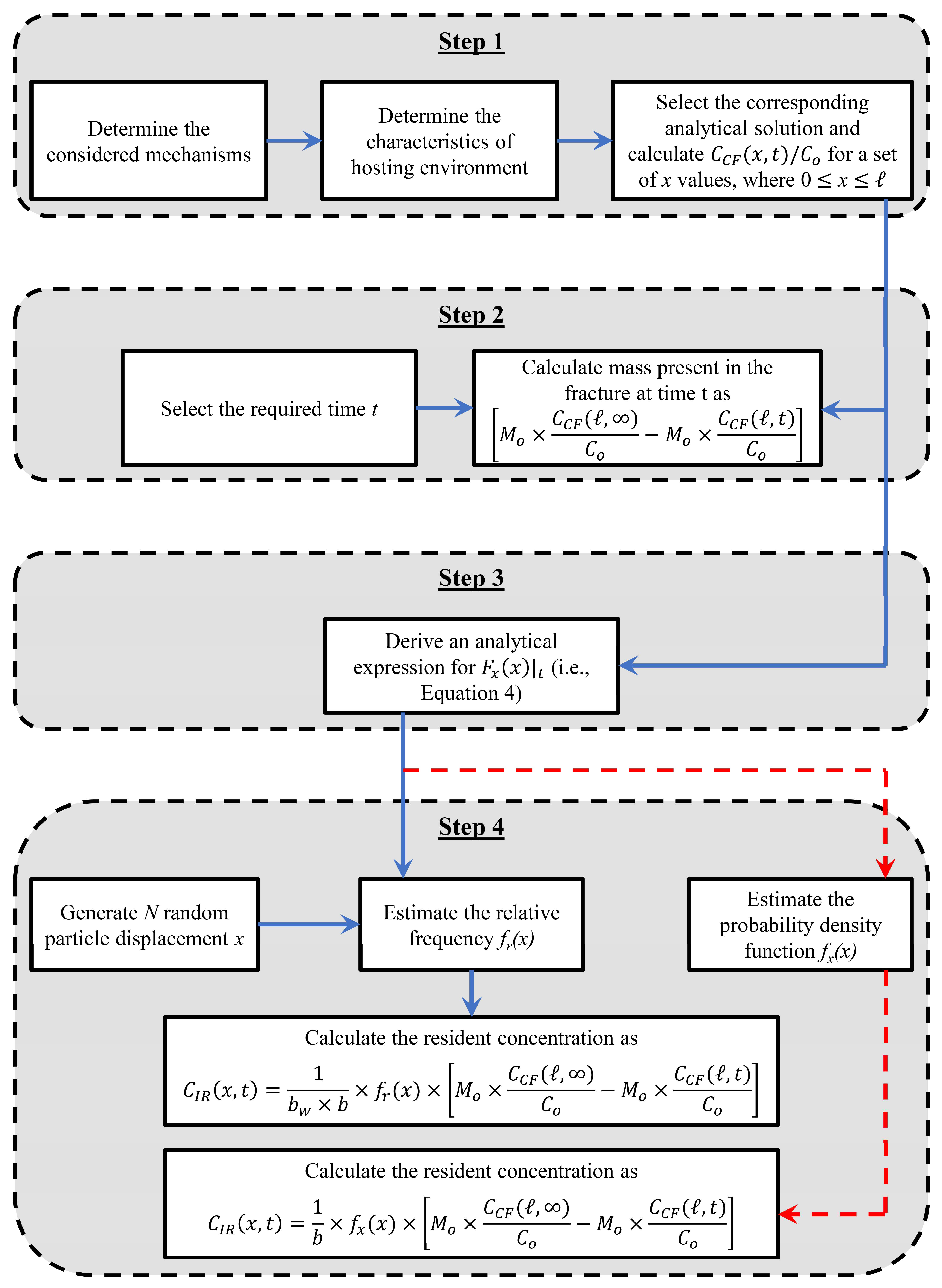
3. The Spatiotemporal Random Walk Approach

The process of concentration mapping in DFNs implies estimating the CP over each fracture within the network. This CP is quantified based on the contaminant mass (i.e., the number of particles) present at a specific location in the fracture. Under an instantaneous injection at the inlet, the number of particles at a specific location reflects the frequency of randomly generated travel distances according to a predetermined probability distribution that considers the different fate and transport mechanisms. The STRW approach presented in this study, thus, relies on using an analytical description for the travel distance’s probability distribution to estimate the CPs in single fractures. The development and application procedure of this analytical description, as well as the application steps of the STRW approach, are discussed in this section and are summarized in in Figure 1.

3.1. Step 1: Identifying the Contaminant Fate and Transport Mechanisms of Interest

As described earlier, several fate and transport mechanisms control the contaminant behavior in single fractures. Different contaminants are affected by related specific mechanisms (e.g., size exclusion for colloids and decay for radionuclides); however, general mechanisms include advection, mechanical dispersion, matrix diffusion, and deposition. Several closed-form expressions were developed to describe contaminant behavior while considering the different mechanisms, including the solution by Bear [70] for solutes in impermeable fractures, by Tang et. al. [20] and Sudiky and Frind [31] for solutes in permeable fractures, and by Abdel-Salam and Chrysikopoulos [26] for particulates in permeable and impermeable fractures. The first step of applying the STRW approach aims at determining the type of contaminant of interest (i.e., identifying the fate and transport mechanism) as well as the characteristics of the hosting environment (e.g., permeable or impermeable solid matrix). Subsequently, an appropriate analytical solution describing contaminant behavior in such environments is selected.

3.2. Step 2: Selecting the Time Instance(s) of Interest and Calculating the Corresponding Mass Present in the Fracture

The second step of applying the STRW approach is to determine a time instance(s) at which the CP is estimated. Such instances of time are selected depending on the purpose of CP calculation or concentration mapping such as preparing a pumping schedule, introducing treatment agents for remediation purposes, or monitoring the spatial evolution of contaminants over time. Following the selection of the time instance(s) of interest, the corresponding amount of contaminant (i.e., mass) present within the fracture is estimated. Such an amount is calculated based on the analytical solution selected in the previous step and is subsequently used for estimating the spatial distribution of the contaminant over the full length of the fracture (i.e., CP calculation, as described in the next seps).

3.3. Step 3: Deriving an Analytical Expression for the Probability Distribution of Particle Displacement

Assuming an impervious single fracture with a length ℓ and an average aperture b, where a contaminant mass M_o is injected instantaneously at the inlet, the mass of contaminant present over the full length of the fracture (M_R) at time t can be estimated as follows:

$$M_R(t)={\int }_0^{\mathcal{l}}{A}_f{C}_{IR}\left(x,t\right)dx$$

(1)

where A_f [L²] is the cross-sectional area of the fracture, C_IR(x,t) [ML⁻³] is the volume-averaged concentration, x [L] is the distance measured from the fracture inlet, and t [T] is the time. The probability distribution function of particle displacement F_x(x) at time t can be accordingly estimated as

$$F_x\left(x\right){|}_t=\frac{{\int }_0^x{A}_f{C}_{IR}\left(x,t\right)dx}{M_R\left(t\right)}.$$

(2)

Kreft and Zuber [33] developed a relationship between C_IR(x,t) and the flux concentration C_IF(x,t) based on the principles of mass conservation at a distance x from the fracture inlet. Such relationship can be represented as follows:

$$C_{IR}\left(x,t\right)=-u\frac{\partial }{\partial x}\left({\int }_0^t{C}_{IF}\left(x,t\text{'}\right)dt\text{'}\right)$$

(3)

where u [LT⁻¹] is the flow velocity within the fracture. It should be noted that the integral in Equation (3) can be represented in terms of the flux concentration, assuming a continuous injection with intensity C_o at the fracture inlet as detailed in [33]. As such, through combining Equations (1)–(3) and using the axiom that $\frac{{uA}_f{C}_o}{M_o}\times {\int }_0^t{C}_{IF}\left(0,t\text{'}\right)dt\text{'}=C_o$, Equation (2) can be replaced by

$$F_x\left(x\right){|}_t=\frac{1-\frac{C_{CF}(x,t)}{C_o}}{1-\frac{C_{CF}(\mathcal{l},t)}{C_o}}$$

(4)

where C_CF(x,t) [ML⁻³] is the flux concentration, assuming a continuous injection of C_o at the fracture inlet. It should be emphasized that several closed-form expressions have been developed to evaluate C_CF(x,t)/C_o for one-dimensional flow conditions while considering a wide spectrum of fate and transport mechanisms, including advection, dispersion, and reversible deposition [70]; irreversible deposition [26]; and matrix diffusion [20,31], as described in Step 1 of the application procedures of the STRW approach. As such, Equation (4) represents a general analytical description for the statistical behavior of particle displacement in fractures under instantaneous injection. It should be highlighted that this analytical description also inherits the same assumptions used for developing the closed-form expressions of C_CF(x,t)/C_o.

It should be reiterated that Equation (4) was derived based on the assumption that contaminant mass is introduced instantly at the fracture inlet. Closed forms of Equation (4) (i.e., analytical expressions for F_x(x)) are, thus, presented in Section 4 for a range of mechanisms under which analytical descriptions of C_CF(x,t)/C_o are currently available as well as closed-form expressions for C_IR(x,t) that can be developed for comparison purposes. However, extending the applicability of the STRW approach to time-dependent injection at the inlet is described in Section 5 when the method is applied in DFNs.

3.4. Step 4: Estimating the CP

For concentration mapping (i.e., estimating the CP) in single fractures, a number of N particles are assumed to enter the fracture, and each is assigned a random displacement based on the analytical description of F_x(x) developed in Step 3. The relative frequency of particle displacement, f_r(x), is subsequently estimated, and the mass present within the fracture (determined in Step 2) is then fractioned among the histogram bins based on the corresponding relative frequency. The volume-averaged concentration, C_IR(x,t), is finally calculated over the fracture length at the selected times as the mass present within segmented volumes of the fracture as shown in Figure 1, and the corresponding C_IF(x,t) can also be calculated using the transformations presented in Kreft and Zuber [33]. It should be noted that the probability density function for particle displacement, f_x(x), can be used instead of the relative frequency and can be subsequently used for C_IR(x,t) and C_IF(x,t) calculations, as shown in Figure 1. Such a density function can be calculated through an analytical or algorithmic (i.e., automatic) differentiation procedure.

Figure 1. A flow chart describing the application procedure of the developed STRW approach in single fractures under an instantaneous influent injection. It should be noted that the estimation of C_IR(x,t) in Step 4 can be achieved through the calculation of f_r(x) or f_x(x) following the process represented by the red and blue arrows, respectively, where b_w is the bin size used for relative frequency calculation.

Figure 1. A flow chart describing the application procedure of the developed STRW approach in single fractures under an instantaneous influent injection. It should be noted that the estimation of C_IR(x,t) in Step 4 can be achieved through the calculation of f_r(x) or f_x(x) following the process represented by the red and blue arrows, respectively, where b_w is the bin size used for relative frequency calculation.

4. Method Verification in Single Fractures

Four different cases were designed to demonstrate the efficacy of the STRW approach in mapping the contaminant concentration in single fractures by assuming the following: (i) the fracture walls can be represented as two parallel plates with a unit width; (ii) steady state flow conditions are fully developed within the fracture; (iii) the contaminant is released instantaneously at the inlet; (iv) particles are not sorbed to the solid matrix when matrix diffusion is considered. The fate and transport mechanisms as well as the analytical solutions (in terms of flux concentration) used for comparison in such verification cases are provided in

Table 1. Fate and transport mechanisms and corresponding analytical solution used within the different verification cases in single fractures.

Verification Case	Fate and Transport Mechanisms Considered	Reference for the Corresponding Analytical Solution
Case 1	Advection, dispersion, and reversible deposition	[70]
Case 2	Advection, dispersion, and irreversible deposition	[26]
Case 3	Advection, dispersion, and matrix diffusion	[20]
Case 4	Advection, size-dependent dispersion, and irreversible deposition	[71]

, whereas a detailed description of each case is provided in the following subsections. It should be highlighted that, in all verification cases, the STRW approach was applied using 10,000 particles and was embedded within a Monte Carlo simulation of 1000 realizations in order to minimize the noise typically associated with estimates from random walk approaches. The ensemble CPs are subsequently used as represented solutions. It should be also mentioned that three instances of time were selected in all verification cases for comparison purposes. Such time instances represent 50%, 100%, and 150% of the corresponding advection time in the fracture (i.e., ℓ/u).

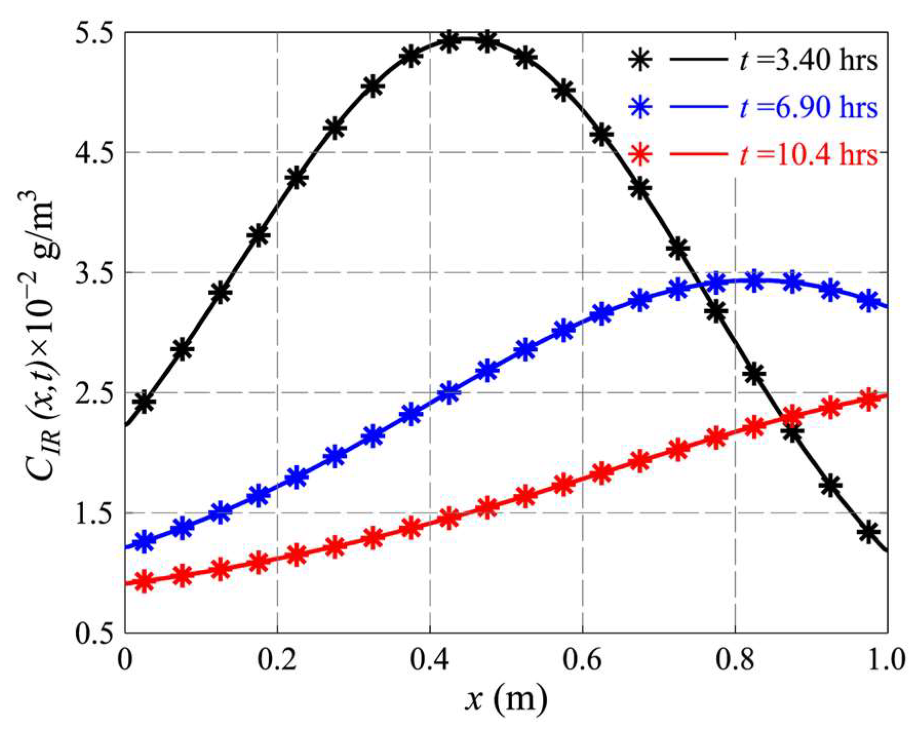
4.1. Case 1: Advection, Dispersion, and Reversible Deposition in Single Fractures

This verification case was selected to verify the applicability of the STRW approach under a set of primary transport mechanisms (i.e., advection, dispersion, and reversible deposition). Under advection and dispersion only, Ogata and Banks [72] developed an analytical description for C_CF(x,t)/C_o in semi-infinite single fractures, which can be adjusted to account for linear, equilibrium, reversible deposition using a retardation factor R. Under such adjustment, the solution by Ogata and Banks [72] can be represented as in Equation (5), whereas F_x(x) can be described analytically using Equation (6):

$$\frac{C_{CF}\left(x,t\right)}{C_o}=\frac{1}{2}\left[erfc\left(\frac{x-\frac{ut}{R}}{\sqrt{4Dt}}\right)+exp \left(\frac{ux}{RD}\right)erfc\left(\frac{x+\frac{ut}{R}}{\sqrt{4Dt}}\right)\right],$$

(5)

$$F_x\left(x\right){|}_t=\frac{2-erfc\left(\frac{x-\frac{ut}{R}}{\sqrt{4Dt}}\right)-exp \left(\frac{ux}{RD}\right)erfc\left(\frac{x+\frac{ut}{R}}{\sqrt{4Dt}}\right)}{2-erfc\left(\frac{\mathcal{l}-\frac{ut}{R}}{\sqrt{4Dt}}\right)-exp \left(\frac{u\mathcal{l}}{RD}\right)erfc\left(\frac{\mathcal{l}+\frac{ut}{R}}{\sqrt{4Dt}}\right)}.$$

(6)

The STRW approach can subsequently be applied after replacing Equation (4) in Figure 1 with Equation (6). As previously discussed, the STRW approach typically results in CPs based on the volume-averaged concentration. However, analytical solutions for contaminant transport in single fractures under instantaneous injection at the inlet considering advection, dispersion, and reversible deposition are available in terms of the flux concentration [70]. As such, and to facilitate evaluating the performance of the STRW approach in this verification case, the analytical solution reported in Bear [70] is transformed into a volume-averaged-concentration-based formula using Equation (3). The resulting analytical description for C_IR(x,t) is represented by Equation (7), and CP estimates based on this equation are subsequently compared to those resulting from the STRW approach.

$$C_{IR}\left(x,t\right)=\frac{M_{o}u}{Q\sqrt{4\pi Dt}}\left[\frac{{2e}^{-\frac{{\left(x-ut\right)}^2}{4Dt}}}{\sqrt{4Dt}}-u\sqrt{\frac{\pi t}{D}}erfc\left(\frac{x+ut}{\sqrt{4Dt}}\right)\right]$$

(7)

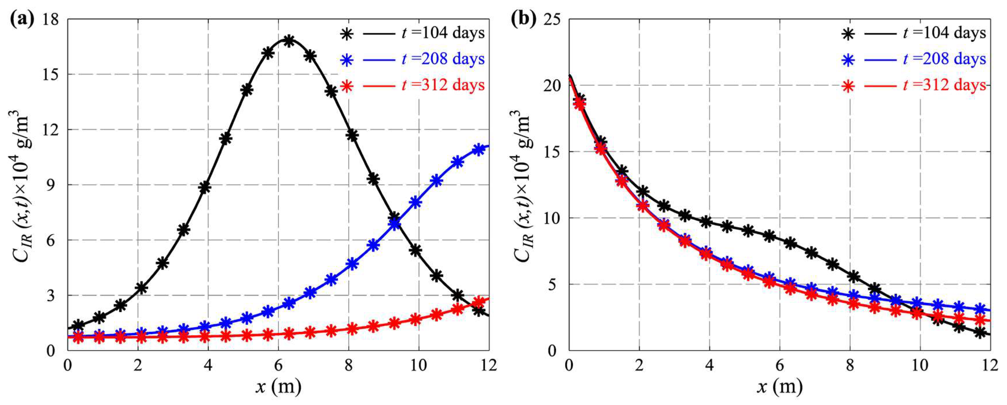
4.2. Case 2: Advection, Dispersion, and Irreversible Deposition in Single Fractures

This case was devised to test the ability of the STRW approach to emulate the spatial aspect of colloid behavior in single fractures, where irreversible deposition is documented as the primary retention mechanism [73,74,75]. Under continuous injection at the fracture inlet, Abdel-Salam and Chrysikopoulos [26] developed an analytical formula to estimate C_CF(x,t)/C_o in semi-infinite impervious fractures. Such an analytical formula can be used to derive a corresponding closed-form expression for F_x(x). The analytical solution developed by Abdel-Salam and Chrysikopoulos [26] as well as that of F_x(x) can be, respectively, represented as follows:

$$\frac{C_{CF}\left(x,t\right)}{C_o}=\frac{1}{2}{e}^{\frac{ux}{2D}}\left[e^{-\frac{ux}{2D}\xi }erfc\left(\frac{x-ut\xi }{\sqrt{4Dt}}\right)+e^{\frac{ux}{2D}\xi }erfc\left(\frac{x+ut\xi }{\sqrt{4Dt}}\right)\right],$$

(8)

$$F_x\left(x\right){|}_t=\frac{2-e^{\frac{ux}{2D}}\left[e^{-\frac{ux}{2D}\xi }erfc\left(\frac{x-ut\xi }{\sqrt{4Dt}}\right)+e^{\frac{ux}{2D}\xi }erfc\left(\frac{x+ut\xi }{\sqrt{4Dt}}\right)\right]}{2-e^{\frac{u\mathcal{l}}{2D}}\left[e^{-\frac{u\mathcal{l}}{2D}\xi }erfc\left(\frac{\mathcal{l}-ut\xi }{\sqrt{4Dt}}\right)+e^{\frac{u\mathcal{l}}{2D}\xi }erfc\left(\frac{\mathcal{l}+ut\xi }{\sqrt{4Dt}}\right)\right]}$$

(9)

where ξ is evaluated in terms of the lumped deposition coefficient (κ) as $\xi =\sqrt{1+\frac{8\kappa D}{u{b}^2}}$. Similar to Case 1, the STRW can be applied after replacing Equation (4) with Equation (9). In addition, the analytical solution developed by Abdel-Salam and Chrysikopoulos [26], represented by Equation (8), was used to derive a closed-form expression for C_IR(x,t) based on the transformation provided in [33] to facilitate the comparison to the STRW-based CPs. This transformed analytical expression of C_IR(x,t) can be written as

$$C_{IR}\left(x,t\right)=\frac{M_{o}u}{Q}\left[\frac{e^{-\frac{{\left(x-ut\xi \right)}^2}{4Dt}}}{\sqrt{4Dt}}+\frac{e^{-\frac{{\left(x+ut\xi \right)}^2}{4Dt}}}{\sqrt{4Dt}}-\frac{u\left(1-\xi \right)}{4D}erfc\left(\frac{x-ut\xi }{\sqrt{4Dt}}\right)-\frac{u\left(1+\xi \right)}{4D}erfc\left(\frac{x+ut\xi }{\sqrt{4Dt}}\right)\right].$$

(10)

4.3. Case 3: Advection, Dispersion, and Matrix Diffusion in Single Fracture–Matrix Systems

Matrix diffusion is a slow process through which particles transfer between open fractures and the soil matrix due to concentration gradient across the fracture walls. Although some particles may become trapped within the matrix, matrix diffusion has typically been simulated as a reversible process that results in delayed and heavy-tailed BTCs. Tang et al. [20] developed an analytical solution for C_CF(x,t)/C_o in single fractures when matrix diffusion is considered. When only matrix diffusion, advection, and dispersion are of interest, the analytical solution can be expressed as

$$\frac{C_{CF}\left(x,t\right)}{C_o}=\frac{2\times exp\left(\frac{ux}{2D}\right)}{\sqrt{\pi }}\times {\int }_{\frac{x}{\sqrt{4Dt}}}^{\infty }exp\left(-\frac{u^2{x}^2+16D^2{\tau }^4+4D{x}^2}{16D^2{\tau }^2}\right)erfc\left(\frac{\theta x^2\sqrt{D_e}}{4bD{\tau }^2\sqrt{t-\frac{x^2}{4D{\tau }^2}}}\right)d\tau$$

(11)

where τ [−] is a dummy variable used for evaluating the integral in Equation (11), θ [−] is the matrix porosity, and D_e [L²T⁻¹] is the effective diffusion coefficient in the matrix. When Equations (4) and (11) are coupled, an analytical description of F_x(x) can be developed for the stochastic behavior of particle displacement in single fractures under the considered mechanisms. To facilitate the comparison in this verification case, CPs estimated using the analytical solution reported by Tang et al. [20] were directly converted into volume-averaged concentration, as detailed in [33], and were subsequently compared to the STRW-based CPs.

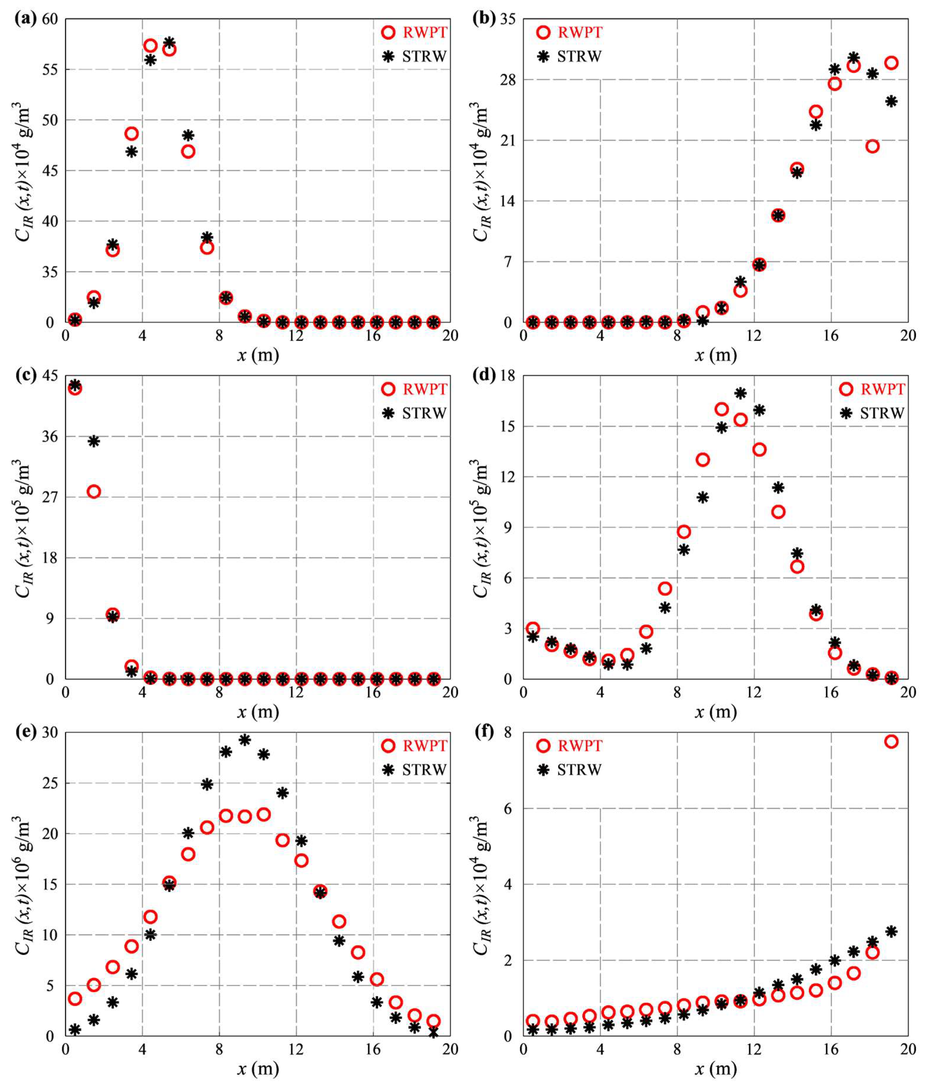
4.4. Case 4: Advection, Size-Dependent Dispersion, and Irreversible Deposition in Single Fractures

Colloids existing in groundwater may have different sizes that can be described statistically using a lognormal distribution [32,76]. Accordingly, the aggregated behavior of a plume of polydisperse colloids depends on the intrinsic transport mechanisms of each particle. In such a case, colloid deposition has been described through the dimensionless Damköhler number (D_a), which is related to the lumped deposition coefficient, κ, as $D_a=12\kappa u/(12D_e-2\kappa u)$ [55]. As the diffusion coefficient (i.e., D_e) is a function of the particle size (d), both the particle dispersion and deposition are not consistent for all particles within the plume. James and Chrysikopoulos [71] developed analytical solutions for polydispersed colloid behavior in semi-infinite single fractures under a set of injection schemes at the inlet. For continuous colloid release at the fracture inlet, the analytical solution by James and Chrysikopoulos [71] is expressed in terms of the flux concentration:

$$\frac{C_{CF}\left(x,t\right)}{C_o}=\frac{1}{2}{\int }_0^{\infty }{f}_d\left(d\right)\mathit{exp}\left(\frac{U_{eff}x}{2D_{eff}}\right)\times \left[\exp \left(-\frac{\Omega x}{2D_{eff}}\right)erfc\left(\frac{x-\Omega t}{\sqrt{4D_{eff}t}}\right)+\exp \left(\frac{\Omega x}{2D_{eff}}\right)erfc\left(\frac{x+\Omega t}{\sqrt{4D_{eff}t}}\right)\right]$$

(12)

where f_d(d) [−] is the probability density function of particle size, $\Omega =\sqrt{U_{eff}^2+4K_{eff}{D}_{eff}}$, and U_eff [LT⁻¹], D_eff [L²T⁻¹], and K_eff [T⁻¹] are the effective velocity, dispersion coefficient, and first order decay coefficient, respectively, for a plume of polydisperse colloids undergoing irreversible deposition [71]. It should be highlighted that U_eff, D_eff, and K_eff are all size-dependent and, thus, coupling Equations (4) and (12) results in a complex analytical expression for F_x(x) that is not easy to employ. Alternatively, when the STRW approach is applied in this case, each particle in the plume can migrate within the fracture according to a particle-specific F_x(x) calculated using Equation (9), albeit employing corresponding size-dependent U_eff, D_eff, and K_eff values. The total CP is subsequently estimated as the summation of those based on single particles (i.e., particle-based CPs are estimated similarly to those in Case 2 using the corresponding mass injected). Similar to other verification cases, analytical CPs are estimated using Equation (12), are converted into volume-averaged concentrations, and are subsequently compared to those estimated using the STRW approach.

5. Method Application in Discrete Fracture Networks

As shown in Figure 1, the application of the STRW approach requires identifying the following: (i) the mass existing within the fracture (or the fracture–matrix system) at time t, $M_o\left[\raisebox{1ex}{$C(\mathcal{l},\mathcal{\infty })$}\!\left/ \!\raisebox{-1ex}{$C_o$}\right.-\raisebox{1ex}{$C(\mathcal{l},t)$}\!\left/ \!\raisebox{-1ex}{$C_o$}\right.\right]$; (ii) the relative frequency or probability density function of particle displacement at time t (i.e., f_r(x) or f_x(x), respectively). Therefore, the application of the STRW approach in a DFN requires prior identification of the BTCs at the network’s junctions. This can be achieved through the application of available techniques (e.g., the TDRW [62] or the convolution [56] methods). In addition, most of the fractures in a DFN are subjected to temporal contaminant release at their inlets. As such, the direct application of the STRW approach using Equation (4) is not appropriate.

Conceptualizing temporal contaminant release at the inlet as injecting a small mass ΔM at time W, the corresponding probability distribution function of particle displacement for those within the mass ΔM can be described using Equation (4). This implies discretizing the temporal contaminant release at the inlet into a set of regions with equal mass or concentrations depending on whether the release regime is described in terms of mass or concentration, respectively. The full distribution of particle displacement considering the temporal contaminant injection can be subsequently evaluated through

$$F_x\left(x\right){|}_t={\int }_{t_i}^t\left[\frac{1-f\left(W\right)\times \frac{C_{CF}(x,t-W)}{C_o}}{1-f\left(W\right)\times \frac{C_{CF}(\mathcal{l},t-W)}{C_o}}\right]dW$$

(13)

where t_i [T] is the initial time of injection and f(W) is the function describing the temporal contaminant release at the fracture inlet. The integral in Equation (13) cannot be evaluated analytically in most cases, hindering the application of the STRW approach in DFNs. Alternatively, estimating the CP in fractures considering a temporal contaminant release at the fracture inlet can be achieved through the following: (1) replacing the total mass injected by a set of n particles, each of which is released at time W_i; (2) estimating the CP at time t due to particle i following the same procedures described in Figure 1, albeit after replacing t with $t-W_i$ in Equation (4); (3) evaluating the total CP over the fracture through location-based summation. In order to map the contaminant concentration over the whole DFN, these steps are repeated for every fracture where the contaminant may exist at time t. Determining this set of fractures, thus, requires scanning the BTCs at all junctions of the network and subsequently determine the fractures that contain a mass fraction at time t.

6. Results and Discussion

For verification Case 1, the STRW-based CPs were estimated at 1.4, 2.9, and 4.3 days assuming the following parameters: M_o = 10⁻³ g, u = 4 × 10⁻⁵ m/s, D = 2 × 10⁻⁵ m²/s, b = 2.5 × 10⁻⁴ m, ℓ = 10 m, and R = 1.2 [62]. It should be noted that the values of these parameters are similar to those employed in the study by Bodin et. al. [62]. The STRW-based CPs were subsequently compared to those estimated using Equation (7). As shown in Figure 2, the STRW approach effectively replicated the analytical CPs with normalized root mean squared error (NRMSE) values of 3 × 10⁻³, 1 × 10⁻³, and 7 × 10⁻⁴ at 1.4, 2.9, and 4.3 days, respectively. In addition, the STRW approach could efficiently support the intuitive understanding of the temporal contaminant behavior in fractures, where the mass present within the fracture reduces over time. This mass can be indicated by the area under the CP, which decreases as the time increases, as shown in Figure 2. It should be noted that the NRMSE values used for CP comparison were estimated through using corresponding maximum analytical concentrations as normalization factors.

In verification Case 2, a groundwater–colloid–fracture system with u = 1 m/year, D = 0.25 m²/year, b = 125 × 10⁻⁶ m, ℓ = 5 m, κ/b² = 6.4 × 10⁻³, and 3.2 × 10⁻² m⁻¹ was employed [26], and the STRW-based CPs were estimated at 2.5, 5, and 7.5 years. Similar parameter values were employed by Abdel-Salam and Chrysikopoulos [26]. As shown in Figure 3, the STRW-based CPs perfectly matched those estimated using Equation (10), with NRMSE values at 2.5, 5, and 7.5 years of 1.3 × 10⁻³, 7.1 × 10⁻⁴, and 6 × 10⁻⁴ for κ/b² equals 6.4 × 10⁻³ m⁻¹ and 1.2 × 10⁻³, 8.6 × 10⁻⁴, and 1.1 × 10⁻³ when κ/b² is 3.2 × 10⁻² m⁻¹. In addition to conserving the mass balance principles (i.e., contaminant mass within the fracture decreases over time under instantaneous injection at the inlet), the STRW approach efficiently preserved the conceptual impact of irreversible deposition (i.e., reduced peaks under higher deposition levels).

When matrix diffusion is considered in verification Case 3, a fracture–matrix system of ℓ = 1 m, b = 2.5 × 10⁻⁴ m, u = 4 × 10⁻⁵ m/s, D = 4 × 10⁻⁶ m²/s, θ = 0.05, and D_e = 5 × 10⁻¹¹ m²/s was employed [27], and 10⁻⁵ g of a conservative contaminant was released instantaneously at the inlet. Similar parameter values were employed by Delay and Bodin [27]. Analytical and STRW-based CPs were subsequently estimated at 3.4, 6.9, and 10.4 h, and the STRW approach efficiently replicated the CPs evaluated analytically (based on the transformation of Equation (11)) as shown in Figure 4. The NRMSE values were 9.8 × 10⁻⁴, 1 × 10⁻³, and 7.5 × 10⁻⁴ at 3.4, 6.9, and 10.4 h, respectively. Similar to verification Case 1, the STRW approach efficiently preserved the principles of mass conservation, where the contaminant mass present within the fracture (indicated by the area under the CP) decreases over time.

In verification Case 4, a plume of polydisperse colloids with a total mass of 100 g is released instantly at the fracture inlet. The colloid diameter is assumed to follow a lognormal distribution with a mean and standard deviation of 1 μm and 0.9 μm, respectively [71]. A single D_a value was assigned to the colloid plume, implying that each particle follows a different deposition regime (as D_a is a function of D_e and κ). The fracture characteristics employed in this verification case were ℓ = 12 m, b = 1 × 10⁻⁴ m, and u = 6.7 × 10⁻⁷ m/s [71], and the groundwater flowing within the fracture was assumed to be at 20 °C. It should be noted that similar parameter values were adopted in the study by James and Chrysikopoulos [71]. The STRW approach efficiently reproduced the CPs estimated based on the transformation of the analytical solution presented in Equation (12) at 104, 208, and 312 days, as shown in Figure 5. At the three instances of time, the NRMSE values were 7.3 × 10⁻³, 6 × 10⁻³, and 17.6 × 10⁻³ at a D_a value of 1 × 10^−4.5 and were 2.3 × 10⁻², 2.4 × 10⁻², and 2.5 × 10⁻² at a D_a value of 1 × 10⁻³. At the different deposition levels (i.e., D_a values), the STRW approach also preserved the principles of mass conservations, where the mass present within the fracture (i.e., indicated by the area under the CP) is observed to decrease over time, as shown in Figure 5.

The results presented above support the efficacy of the STRW approach in producing accurate CPs in single fractures for a range of fate and transport mechanisms. It should be reiterated that, as the F_x(x) expressions used for particle displacement generation in single fractures are analytical by-design, assumptions and limitations inherited in the underlying analytical solutions (describing contaminant fate and transport) are directly transferable to F_x(x). Despite the proven efficacy of the STRW approach in single fractures, extending its application to the network scale is of a greater interest. As such, the performance of the STRW approach was tested in the synthetic, impermeable DFN shown in Figure 6. It should be reiterated that, when a fractured aquifer is conceptualized through a set of fractures connected as a network, several DFN realizations are generated based on the stochastic characteristics of the fracture properties (e.g., length, location, orientation, and aperture). As such, the DFN shown in Figure 6 reflects only a single realization of the aquifer’s geometric and hydraulic properties and has been synthesized in this verification case just to demonstrate the efficacy of the STRW approach at the network level. The fracture aperture across the network is assumed to follow a lognormal distribution with a mean and standard deviation of 5 × 10⁻⁶ m and 5 × 10⁻¹² m, respectively (Figure 6a). A total of 100 g of conservative tracer (represented by 10,000 particles) was injected instantaneously along the western boundary of the network, and the STRW approach was applied to map the contaminant concentration over all fractures at 18.4 and 55.2 years. These instances of time represent 50% and 150% of the average total advection time through the network. Injected particles are assigned to fractures connected to the injection (i.e., west) boundary based on the latter’s transmissivity, with a larger number of particles allocated to highly transmissive fractures. Moving through the network, particles are partitioned at fracture intersections, assuming a perfect mixing condition. It should be highlighted that velocities in the fractures range between 0.26 and 7.93 m/year and are calculated based on a 100 m head value at the western boundary, 99 m head value at the eastern boundary, and no-flow condition at both the northern and southern boundaries (Figure 6b). A constant dispersivity of 0.25 m is also assumed in all fractures, and the dispersion coefficient, thus, varies over the fractures based on the corresponding velocity.

For comparison purposes, the RWPT method was also applied to simulate the spatial distribution of contaminant concentration across the same DFN. It should be noted that both the STRW and RWPT methods were applied within a Monte Carlo simulation with 1000 realizations to minimize the expected noise, as described earlier. The STRW-based ensemble CPs matched those estimated using the RWPT method for the selected fractures (Fractures 1, 2, and 3 indicated in Figure 6b) as shown in Figure 7. At the network scale, the predictability of the STRW approach was consistent over time (Figure 8a), supporting the efficacy of the STRW as a concentration mapping tool in DFNs (a sample map is shown in Figure 8b). It should be emphasized that the large deviations between the STRW- and RWPT-based solutions shown in Figure 8a occur in fractures associated with highly dispersive influent BTCs that extend over a large time period. Such BTCs are typically attributed to significantly uncertain particle arrival times described by distributions with a large number of outliers or multimodal distributions. Imitating such a situation necessitates reassembling these BTCs into an immense number of particles. This workaround is challenging when the RWPT method is employed as follows: (i) BTC estimation and concentration mapping are coupled; (ii) the number of particles injected into the network is fixed and is typically predetermined prior to the simulation. In contrast, when the STRW approach is utilized, the number of particles used for concentration mapping may not be similar to that used for BTC estimation, supporting the flexibility of the STRW approach.

The results presented in this study support the efficacy of the STRW approach to accurately map the contaminant concentration in single fractures and DFNs while considering a range of fate and transport mechanisms (i.e., advection, dispersion, matrix diffusion, irreversible deposition, and size-dependent transport). At the network scale and compared to the RWPT method, the STRW is more flexible and efficient: (1) it can easily incorporate several transport mechanisms, as long as a corresponding F_x(x) can be constructed analytically or numerically; (2) its application is considered to be a computational order of O(N_p × N_f) compared to an order of O(N_p × N_f × N_t) when the RWPT method is employed, where N_p is the number of particles, N_f is the number of fractures containing a fraction of contaminant at time t, and N_t is the number of time steps used by each particle to migrate within each fracture when the RWPT method is applied; (3) the use of Monte Carlo simulation can be avoided as F_x(x) can be easily converted into a corresponding density function, f_x(x), through a differentiation process that can be conducted either analytically or numerically. The latter can further enhance the computational efficiency of the STRW approach compared to the RWPT method. However, it should be highlighted that the application of the STRW approach, particularly in DFNs, necessitates a prior estimation of the BTCs at the fracture ends, which is implicitly embedded within the application of the RWPT method. As such, the use of the RWPT method for concentration mapping can be more efficient in DFNs with a fewer number of fractures or when the particle interaction with the fracture surface and solid matrix is significantly rapid (e.g., in case of equilibrium deposition). In contrast, the use of the STRW approach with the prior application of a rapid BTC quantification method (i.e., the TDRW approach and the convolution method) can be more computationally efficient in complex DFNs with larger numbers of intersected fractures or when the particle residence time is significantly large. The latter typically occurs when the impact of matrix diffusion is significant or when complex particle–fracture or particle–matrix interactions are present (e.g., under matrix diffusion or two-site kinetics). However, it should be emphasized that errors inherited in BTCs estimated using the TDRW approach or the convolution method are directly transferable to STRW-based concentration maps (or CPs). When coupled with a proper BTC quantification method, the STRW approach produces CPs and concentration maps that can subsequently be used for the following: (1) developing effective remediation programs through determining optimal locations for treatment wells; (2) identifying possible locations for waste disposal such as landfills and deep geological repositories; (3) estimating the potential contamination risk, which can support urban development activities.

7. Conclusions

This study describes the development of an analytically enhanced Spatiotemporal Random Walk (STRW) approach that can be utilized to accurately map the time-dependent contaminant concentration in single fractures and Discrete Fracture Networks (DFNs). The core of the STRW approach is a distribution function that employs existing analytical solutions in single fractures to describe the stochastic behavior of particle displacement in single fractures and DFNs. Four verification cases were designed to evaluate the performance of the STRW approach in single fractures. The normalized root mean squared error (NRMSE) was used as an error estimator to evaluate the deviation of STRW-based concentration profiles (CPs) from those estimated using corresponding analytical solutions. The four verification cases included contaminant transport under the following conditions: (1) advection, dispersion, and reversible deposition; (2) advection, dispersion, and irreversible deposition; (3) advection, dispersion, and matrix diffusion; (4) advection, size-dependent dispersion, and irreversible deposition. In all of the four verification cases, the STRW approach efficiently reproduced the corresponding analytical CPs at different instances of time while considering different parameter levels with NRMSE values ranging between 6 × 10⁻⁴ and 2.5 × 10⁻². At the network scale, the STRW approach efficiently replicated the CPs estimated using the Random Walk Particle Tracking (RWPT) method in a synthetic impermeable DFN at different instances of time. The STRW approach represents a step forward for extending the applicability of analytical solutions developed in single fractures to the network scale, as such solutions are the basis of particle displacement’s distribution function used within the STRW approach. In addition, the STRW approach is a more reliable concentration mapping technique in DFNs, compared to the RWPT method: (i) it requires less computational operations; (ii) its integration with Monte Carlo simulations for noise reduction can be avoided; (iii) it can easily accommodate complex transport mechanisms (e.g., matrix diffusion and two-site kinetics) that are challenging to simulate using the RWPT method. However, it should be noted that the application of the STRW approach in DFNs must be preceded with a breakthrough curve (BTC) quantification process, which can be more computationally efficient in complex DFNs with larger number of interconnected fractures or when complex particle–fracture–matrix interactions are present. Errors inherited in employed BTCs are, thus, directly transferable to STRW-based estimates (i.e., CPs and concentration maps); therefore, efficient BTC quantification methods should be coupled with the STRW approach. Overall, the STRW is an accurate, flexible, and computationally efficient concentration mapping technique that can facilitate the evaluation of the expected contamination risk in fractured aquifers and, thus, aid in the proactive and prompt decision-making process. Concentration maps estimated using the STRW approach can also support the development of efficient operation, management, and remediation strategies for fractured hydrogeological formations when contamination is realized. Future related research can be directed towards the following: (1) investigating the performance of the STRW approach under more complex transport mechanisms (e.g., decay-chain transport and cotransport of multiple contaminants); (2) assessing the utility of the STRW approach for aquifer characterization purposes (e.g., transport pathway identification); (3) evaluating the extension of the STRW to heterogenous porous aquifers.

References

1. Smith, M.; Cross, K.; Paden, M.; Laban, P. Spring—Managing Groundwater Sustainably; IUCN: Gland, Switzerland, 2016; ISBN 9782831717890. [Google Scholar]
2. Zang, Y.; Hou, X.; Li, Z.; Li, P.; Sun, Y.; Yu, B.; Li, M. Quantify the Effects of Groundwater Level Recovery on Groundwater Nitrate Dynamics through a Quasi-3D Integrated Model for the Vadose Zone-Groundwater Coupled System. Water Res. 2022, 226, 119213. [Google Scholar] [CrossRef] [PubMed]
3. Tang, Y.; Hooshyar, M.; Zhu, T.; Ringler, C.; Sun, A.Y.; Long, D.; Wang, D. Reconstructing Annual Groundwater Storage Changes in a Large-Scale Irrigation Region Using GRACE Data and Budyko Model. J. Hydrol. 2017, 551, 397–406. [Google Scholar] [CrossRef]
4. Yosri, A.; Siam, A.; El-Dakhakhni, W.; Dickson-Anderson, S. A Genetic Programming–Based Model for Colloid Retention in Fractures. Groundwater 2019, 57, 693–703. [Google Scholar] [CrossRef] [PubMed]
5. Masciopinto, C.; Passarella, G.; Caputo, M.C.; Masciale, R.; De Carlo, L. Hydrogeological Models of Water Flow and Pollutant Transport in Karstic and Fractured Reservoirs. Water Resour. Res. 2021, 57, 1–17. [Google Scholar] [CrossRef]
6. Haggerty, R.; Sun, J.; Yu, H.; Li, Y. Application of Machine Learning in Groundwater Quality Modeling—A Comprehensive Review. Water Res. 2023, 233, 119745. [Google Scholar] [CrossRef]
7. Yu, X.; Cui, T.; Sreekanth, J.; Mangeon, S.; Doble, R.; Xin, P.; Rassam, D.; Gilfedder, M. Deep Learning Emulators for Groundwater Contaminant Transport Modelling. J. Hydrol. 2020, 590, 125351. [Google Scholar] [CrossRef]
8. Sprocati, R.; Rolle, M. Integrating Process-Based Reactive Transport Modeling and Machine Learning for Electrokinetic Remediation of Contaminated Groundwater. Water Resour. Res. 2021, 57, 1–22. [Google Scholar] [CrossRef]
9. Yoon, S.; Lee, S.; Zhang, J.; Zeng, L.; Kang, P.K. Inverse Estimation of Multiple Contaminant Sources in Three-Dimensional Heterogeneous Aquifers with Variable-Density Flows. J. Hydrol. 2023, 617, 129041. [Google Scholar] [CrossRef]
10. Barati Moghaddam, M.; Mazaheri, M.; Mohammad Vali Samani, J. Inverse Modeling of Contaminant Transport for Pollution Source Identification in Surface and Groundwaters: A Review. Groundw. Sustain. Dev. 2021, 15, 100651. [Google Scholar] [CrossRef]
11. Palau, J.; Marchesi, M.; Chambon, J.C.C.; Aravena, R.; Canals, À.; Binning, P.J.; Bjerg, P.L.; Otero, N.; Soler, A. Multi-Isotope (Carbon and Chlorine) Analysis for Fingerprinting and Site Characterization at a Fractured Bedrock Aquifer Contaminated by Chlorinated Ethenes. Sci. Total Environ. 2014, 475, 61–70. [Google Scholar] [CrossRef]
12. Chinye-Ikejiunor, N.; Iloegbunam, G.O.; Chukwuka, A.; Ogbeide, O. Groundwater Contamination and Health Risk Assessment across an Urban Gradient: Case Study of Onitcha Metropolis, South-Eastern Nigeria. Groundw. Sustain. Dev. 2021, 14, 100642. [Google Scholar] [CrossRef]
13. Agudelo Moreno, L.J.; Zuleta Lemus, D.D.S.; Lasso Rosero, J.; Agudelo Morales, D.M.; Sepúlveda Castaño, L.M.; Paredes Cuervo, D. Evaluation of Aquifer Contamination Risk in Urban Expansion Areas as a Tool for the Integrated Management of Groundwater Resources. Case: Coffee Growing Region, Colombia. Groundw. Sustain. Dev. 2020, 10, 100298. [Google Scholar] [CrossRef]
14. Du, C.; Li, X.; Gong, W. A DFN-Based Framework for Probabilistic Assessment of Groundwater Contamination in Fractured Aquifers. Chemosphere 2023, 337, 139232. [Google Scholar] [CrossRef]
15. Joodavi, A.; Aghlmand, R.; Podgorski, J.; Dehbandi, R.; Abbasi, A. Characterization, Geostatistical Modeling and Health Risk Assessment of Potentially Toxic Elements in Groundwater Resources of Northeastern Iran. J. Hydrol. Reg. Stud. 2021, 37, 100885. [Google Scholar] [CrossRef]
16. Fetter, C.W.; Boving, T.; Kreamer, D. Contaminant Hydrogeology, 3rd ed.; Waveland Press Inc.: Long Grove, IL, USA, 2017; ISBN 0023371358. [Google Scholar]
17. Bekhit, H.M.; El-Kordy, M.A.; Hassan, A.E. Contaminant Transport in Groundwater in the Presence of Colloids and Bacteria: Model Development and Verification. J. Contam. Hydrol. 2009, 108, 152–167. [Google Scholar] [CrossRef] [PubMed]
18. Chrysikopoulos, C.V.; Sotirelis, N.P.; Kallithrakas-Kontos, N.G. Cotransport of Graphene Oxide Nanoparticles and Kaolinite Colloids in Porous Media. Transp. Porous Media 2017, 119, 181–204. [Google Scholar] [CrossRef]
19. Rod, K.; Um, W.; Chun, J.; Wu, N.; Yin, X.; Wang, G.; Neeves, K. Effect of Chemical and Physical Heterogeneities on Colloid-Facilitated Cesium Transport. J. Contam. Hydrol. 2018, 213, 22–27. [Google Scholar] [CrossRef]
20. Tang, D.H.; Frind, E.O.; Sudicky, E.A. Contaminant Transport in Fractured Porous Media: Analytical Solution for a Single Fracture. Water Resour. Res. 1981, 17, 555–564. [Google Scholar] [CrossRef]
21. Rausch, R.; Schafer, W.; Therrien, R.; Wagner, C. Solute Transport Modelling: An Introduction to Models and Solution Strategies; Gebr. Borntraeger Verlagsbuchhandlung: Stuttgart, Germany, 2005; ISBN 3443010555. [Google Scholar]
22. Berre, I.; Doster, F.; Keilegavlen, E. Flow in Fractured Porous Media: A Review of Conceptual Models and Discretization Approaches. Transp. Porous Media 2019, 130, 215–236. [Google Scholar] [CrossRef]
23. Iraola, A.; Trinchero, P.; Karra, S.; Molinero, J. Assessing Dual Continuum Method for Multicomponent Reactive Transport. Comput. Geosci. 2019, 130, 11–19. [Google Scholar] [CrossRef]
24. Freeze, R.A.; Cherry, J.A. Groundwater; Prentice-Hall: Englewood Cliffs, NJ, USA, 1979; ISBN 0133653129. [Google Scholar]
25. Katzourakis, V.E.; Chrysikopoulos, C.V. Two-Site Colloid Transport with Reversible and Irreversible Attachment: Analytical Solutions. Adv. Water Resour. 2019, 130, 29–36. [Google Scholar] [CrossRef]
26. Abdel-Salam, A.; Chrysikopoulos, C.V. Analytical Solutions for One-Dimensional Colloid Transport in Saturated Fractures. Adv. Water Resour. 1994, 17, 283–296. [Google Scholar] [CrossRef]
27. Delay, F.; Bodin, J. Time Domain Random Walk Method to Simulate Transport by Advection-Dispersion and Matrix Diffusion in Fracture Networks. Geophys. Res. Lett. 2001, 28, 4051–4054. [Google Scholar] [CrossRef]
28. Liu, D.; Jivkov, A.P.; Wang, L.; Si, G.; Yu, J. Non-Fickian Dispersive Transport of Strontium in Laboratory-Scale Columns: Modelling and Evaluation. J. Hydrol. 2017, 549, 1–11. [Google Scholar] [CrossRef]
29. Liu, L.; Meng, S.; Li, C. A New Analytical Solution of Contaminant Transport along a Single Fracture Connected with Porous Matrix and Its Time Domain Random Walk Algorithm. J. Hydrol. 2022, 610, 127828. [Google Scholar] [CrossRef]
30. Meng, S.; Liu, L. Solute Transport in Fractured Porous Media: Implementation of the Time Domain Random Walk Algorithm for Different Injection Boundaries. J. Hydrol. 2023, 618, 129209. [Google Scholar] [CrossRef]
31. Sudicky, E.A.; Frind, E.O. Contaminant Transport in Fractured Porous Media: Analytical Solutions for a System of Parallel Fractures. Water Resour. Res. 1982, 18, 1634–1642. [Google Scholar] [CrossRef]
32. James, S.C.; Chrysikopoulos, V. Transport of Polydisperse Colloid Suspensions in a Single Fracture. Water Resour. Res. 1999, 35, 707–718. [Google Scholar] [CrossRef]
33. Kreft, A.; Zuber, A. On the Physical Meaning of the Dispersion Equation and Its Solutions for Different Initial and Boundary Conditions. Chem. Eng. Sci. 1978, 33, 1471–1480. [Google Scholar] [CrossRef]
34. March, R.; Doster, F.; Geiger, S. Assessment of CO2 Storage Potential in Naturally Fractured Reservoirs with Dual-Porosity Models. Water Resour. Res. 2018, 54, 1650–1668. [Google Scholar] [CrossRef]
35. Perina, T. Semi-Analytical Model for Solute Transport in a Three-Dimensional Aquifer with Dual Porosity and a Volumetric Source Term. J. Hydrol. 2022, 607, 127520. [Google Scholar] [CrossRef]
36. Jerbi, C.; Fourno, A.; Noetinger, B.; Delay, F. A New Estimation of Equivalent Matrix Block Sizes in Fractured Media with Two-Phase Flow Applications in Dual Porosity Models. J. Hydrol. 2017, 548, 508–523. [Google Scholar] [CrossRef]
37. Botros, F.E.; Hassan, A.E.; Reeves, D.M.; Pohll, G. On Mapping Fracture Networks onto Continuum. Water Resour. Res. 2008, 44, 1–17. [Google Scholar] [CrossRef]
38. Sweeney, M.R.; Gable, C.W.; Karra, S.; Stauffer, P.H.; Pawar, R.J.; Hyman, J.D. Upscaled Discrete Fracture Matrix Model (UDFM): An Octree-Refined Continuum Representation of Fractured Porous Media. Comput. Geosci. 2020, 24, 293–310. [Google Scholar] [CrossRef]
39. Noetinger, B.; Roubinet, D.; Russian, A.; Le Borgne, T.; Delay, F.; Dentz, M.; de Dreuzy, J.R.; Gouze, P. Random Walk Methods for Modeling Hydrodynamic Transport in Porous and Fractured Media from Pore to Reservoir Scale. Transp. Porous Media 2016, 115, 345–385. [Google Scholar] [CrossRef]
40. Berkowitz, B.; Cortis, A.; Dentz, M.; Scher, H. Modeling Non-Fickian Transport in Geological Formations as a Continuous Time Random Walk. Rev. Geophys. 2006, 44, 1–49. [Google Scholar] [CrossRef]
41. Li, X.; Zhang, Y.; Reeves, D.M.; Zheng, C. Fractional-Derivative Models for Non-Fickian Transport in a Single Fracture and Its Extension. J. Hydrol. 2020, 590, 125396. [Google Scholar] [CrossRef]
42. Yin, M.; Ma, R.; Zhang, Y.; Wei, S.; Tick, G.R.; Wang, J.; Sun, Z.; Sun, H.; Zheng, C. A Distributed-Order Time Fractional Derivative Model for Simulating Bimodal Sub-Diffusion in Heterogeneous Media. J. Hydrol. 2020, 591, 125504. [Google Scholar] [CrossRef]
43. Dong, P.; Yin, M.; Zhang, Y.; Chen, K.; Finkel, M.; Grathwohl, P.; Zheng, C. A Fractional-Order Dual-Continuum Model to Capture Non-Fickian Solute Transport in a Regional-Scale Fractured Aquifer. J. Contam. Hydrol. 2023, 258, 104231. [Google Scholar] [CrossRef]
44. Hu, Y.; Xu, W.; Zhan, L.; Zou, L.; Chen, Y. Modeling of Solute Transport in a Fracture-Matrix System with a Three-Dimensional Discrete Fracture Network. J. Hydrol. 2022, 605, 127333. [Google Scholar] [CrossRef]
45. Lei, Q.; Latham, J.P.; Tsang, C.F. The Use of Discrete Fracture Networks for Modelling Coupled Geomechanical and Hydrological Behaviour of Fractured Rocks. Comput. Geotech. 2017, 85, 151–176. [Google Scholar] [CrossRef]
46. Zimmerman, R.W.; Chen, G.; Hadgu, T.; Bodvarsson, G.S. A Numerical Dual-porosity Model with Semianalytical Treatment of Fracture/Matrix Flow. Water Resour. Res. 1993, 29, 2127–2137. [Google Scholar] [CrossRef]
47. Berkowitz, B. Characterizing Flow and Transport in Fractured Geological Media: A Review. Adv. Water Resour. 2002, 25, 861–884. [Google Scholar] [CrossRef]
48. Svensson, U. A Continuum Representation of Fracture Networks. Part I: Method and Basic Test Cases. J. Hydrol. 2001, 250, 170–186. [Google Scholar] [CrossRef]
49. Ahmed, M.I.; Abd-Elmegeed, M.A.; Hassan, A.E. Modelling Transport in Fractured Media Using the Fracture Continuum Approach. Arab. J. Geosci. 2019, 12, 172. [Google Scholar] [CrossRef]
50. Makedonska, N.; Hyman, J.D.; Karra, S.; Painter, S.L.; Gable, C.W.; Viswanathan, H.S. Evaluating the Effect of Internal Aperture Variability on Transport in Kilometer Scale Discrete Fracture Networks. Adv. Water Resour. 2016, 94, 486–497. [Google Scholar] [CrossRef]
51. Huang, N.; Zhang, Y.; Han, S. Effects of Topological Properties with Local Variable Apertures on Solute Transport through Three-Dimensional Discrete Fracture Networks. Processes 2023, 11, 3157. [Google Scholar] [CrossRef]
52. Yosri, A.; Dickson-Anderson, S.; Siam, A.; El-Dakhakhni, W. Transport Pathway Identification in Fractured Aquifers: A Stochastic Event Synchrony-Based Framework. Adv. Water Resour. 2021, 147, 103800. [Google Scholar] [CrossRef]
53. Somogyvári, M.; Jalali, M.; Jimenez Parras, S.; Bayer, P. Synthetic Fracture Network Characterization with Transdimensional Inversion. Water Resour. Res. 2017, 53, 5104–5123. [Google Scholar] [CrossRef]
54. Bodin, J.; Porel, G.; Delay, F.; Ubertosi, F.; Bernard, S.; de Dreuzy, J.R. Simulation and Analysis of Solute Transport in 2D Fracture/Pipe Networks: The SOLFRAC Program. J. Contam. Hydrol. 2007, 89, 1–28. [Google Scholar] [CrossRef]
55. Yosri, A.; Dickson-Anderson, S.; El-Dakhakhni, W. A Modified Time Domain Random Walk Approach for Simulating Colloid Behavior in Fractures: Method Development and Verification. Water Resour. Res. 2020, 56, 1–15. [Google Scholar] [CrossRef]
56. Khafagy, M.; El-Dakhakhni, W.; Dickson-Anderson, S. Analytical Model for Solute Transport in Discrete Fracture Networks: 2D Spatiotemporal Solution with Matrix Diffusion. Comput. Geosci. 2022, 159, 104983. [Google Scholar] [CrossRef]
57. Rhodes, M.E.; Blunt, M.J. An Exact Particle Tracking Algorithm for Advective-Dispersive Transport in Networks with Complete Mixing at Nodes. Water Resour. Res. 2006, 42, 1–7. [Google Scholar] [CrossRef]
58. Wang, L.; Cardenas, M.B. An Efficient Quasi-3D Particle Tracking-Based Approach for Transport through Fractures with Application to Dynamic Dispersion Calculation. J. Contam. Hydrol. 2015, 179, 47–54. [Google Scholar] [CrossRef] [PubMed]
59. Khafagy, M.M.; Abd-Elmegeed, M.A.; Hassan, A.E. Simulation of Reactive Transport in Fractured Geologic Media Using Random-Walk Particle Tracking Method. Arab. J. Geosci. 2020, 13, 34. [Google Scholar] [CrossRef]
60. Hassan, A.E.; Cushman, J.H.; Delleur, J.W. Monte Carlo Studies of Flow and Transport in Fractal Conductivity Fields: Comparison with Stochastic Perturbation Theory. Water Resour. Res. 1997, 33, 2519–2534. [Google Scholar] [CrossRef]
61. Banton, O.; Delay, F.; Porel, G. A New Time Domain Random Walk Method for Solute Transport in 1-D Heterogeneous Media. Groundwater 1997, 35, 1008–1013. [Google Scholar] [CrossRef]
62. Bodin, J.; Porel, G.; Delay, F. Simulation of Solute Transport in Discrete Fracture Networks Using the Time Domain Random Walk Method. Earth Planet. Sci. Lett. 2003, 208, 297–304. [Google Scholar] [CrossRef]
63. Wei, Y.; Chen, J. DFNSC: A Particle Tracking Discrete Fracture Network Simulator Considering Successive Spatial Correlation. Comput. Geotech. 2021, 135, 104156. [Google Scholar] [CrossRef]
64. Salamon, P.; Fernàndez-Garcia, D.; Gómez-Hernández, J.J. A Review and Numerical Assessment of the Random Walk Particle Tracking Method. J. Contam. Hydrol. 2006, 87, 277–305. [Google Scholar] [CrossRef]
65. Majumder, P.; Eldho, T.I. Reactive Contaminant Transport Simulation Using the Analytic Element Method, Random Walk Particle Tracking and Kernel Density Estimator. J. Contam. Hydrol. 2019, 222, 76–88. [Google Scholar] [CrossRef]
66. Hassan, A.E.; Mohamed, M.M. On Using Particle Tracking Methods to Simulate Transport in Single-Continuum and Dual Continua Porous Media. J. Hydrol. 2003, 275, 242–260. [Google Scholar] [CrossRef]
67. Pan, L.; Bodvarsson, G.S. Modeling Transport in Fractured Porous Media with the Random-Walk Particle Method: The Transient Activity Range and the Particle Transfer Probability. Water Resour. Res. 2002, 38, 16-1–16-17. [Google Scholar] [CrossRef]
68. Cvetkovic, V.; Selroos, J.O.; Cheng, H. Transport of Reactive Tracers in Rock Fractures. J. Fluid Mech. 1999, 378, 335–356. [Google Scholar] [CrossRef]
69. Hassan, A.; Pohlmann, K.; Chapman, J. Uncertainty Analysis of Radionuclide Transport in a Fractured Coastal Aquifer with Geothermal Effects. Transp. Porous Media 2001, 43, 107–136. [Google Scholar] [CrossRef]
70. Bear, J. Dynamics of Fluids in Porous Media; American Elsevier: New York, NY, USA, 1972. [Google Scholar]
71. James, S.C.; Chrysikopoulos, C.V. Analytical Solutions for Monodisperse and Polydisperse Colloid Transport in Uniform Fractures. Colloids Surf. A Physicochem. Eng. Asp. 2003, 226, 101–118. [Google Scholar] [CrossRef]
72. Ogata, A.; Banks, R.B. A Solution of the Differential Equation of Longitudinal Dispersion in Porous Media; Report No. 411-A; United States Government Printing Office: Washington, DC, USA, 1961. [CrossRef]
73. Cohen, M.; Weisbrod, N. Transport of Iron Nanoparticles through Natural Discrete Fractures. Water Res. 2018, 129, 375–383. [Google Scholar] [CrossRef] [PubMed]
74. Rodrigues, S.; Dickson, S. A Phenomenological Model for Particle Retention in Single, Saturated Fractures. Groundwater 2014, 52, 277–283. [Google Scholar] [CrossRef] [PubMed]
75. Stoll, M.; Huber, F.M.; Schill, E.; Schäfer, T. Parallel-Plate Fracture Transport Experiments of Nanoparticulate Illite in the Ultra-Trace Concentration Range Investigated by Laser-Induced Breakdown Detection (LIBD). Colloids Surf. A Physicochem. Eng. Asp. 2017, 529, 222–230. [Google Scholar] [CrossRef]
76. Ledin, A.; Karlsson, S.; Düker, A.; Allard, B. Measurements in Situ of Concentration and Size Distribution of Colloidal Matter in Deep Groundwaters by Photon Correlation Spectroscopy. Water Res. 1994, 28, 1539–1545. [Google Scholar] [CrossRef]
Figure 2. Comparison between the STRW-based (points) and analytical (lines) concentration profiles in Case 1.
Water 16 01020 g002
Figure 3. Comparison between the STRW-based (points) and analytical (lines) concentration profiles in Case 2 for κ/b2 values of 6.4 × 10⁻³ m−1 (a) and 3.2 × 10⁻² m−1 (b).
Water 16 01020 g003
Figure 4. Comparison between the STRW-based (points) and analytical (lines) concentration profiles in Case 3.
Water 16 01020 g004
Figure 5. Comparison between the STRW-based (scatter points) and analytical (solid lines) concentration profiles in Case 4 for Da values of 1 × 10−4.5 (a) and 1 × 10⁻³ (b).
Water 16 01020 g005
Figure 6. The synthetic, impermeable DFN employed in this study: (a) the log aperture distribution; (b) the boundary conditions for the flow problem. The color bar in (a) reflects the log aperture values, and the red and blue colors in (b) represent non-flowing and flowing bonds, respectively.
Water 16 01020 g006
Figure 7. Comparison between the STRW- and RWPT-based CPs for Fracture 1 at 18.4 years (a) and 55.2 years (b), for Fracture 2 at 18.4 years (c) and 55.2 years (d), and for Fracture 3 at 18.4 years (e) and 55.2 years (f).
Water 16 01020 g007
Figure 8. The STRW-based results in the synthetic DFN: (a) NRMSE values at different instances of time; (b) a sample volume-averaged concentration (g/m3) map at 18.4 years where the colors represent the corresponding logarithmic values and the asterisks indicate outliers.
Water 16 01020 g008