Article

Can Short-Term Online-Monitoring Improve the Current WFD Water Quality Assessment Regime? Systematic Resampling of High-Resolution Data from Four Saxon Catchments

1
Institute of Urban and Industrial Water Management, Technische Universität Dresden, 01069 Dresden, Germany
2
Beijing Insights Value Technology Co., Ltd., Beijing 100070, China
*
Author to whom correspondence should be addressed.
Water 2024, 16(6), 889; https://doi.org/10.3390/w16060889
Submission received: 20 February 2024 / Revised: 13 March 2024 / Accepted: 14 March 2024 / Published: 20 March 2024
(This article belongs to the Special Issue Field Methods for Water Quality Surveying, Volume II)

Abstract

:
The European Union Water Framework Directive (2000/60/EC; WFD) aims to achieve a good ecological and chemical status of all bodies of surface water by 2027. The development of integrated guidance on surface water chemical monitoring (e.g., WFD Guidance Document No. 7/19) has been transferred into national German law (Ordinance for the Protection of Surface Waters, OGewV). For the majority of compounds, this act requires monthly sampling to assess the chemical quality status of a body of surface water. To evaluate the representativeness of the sampling strategy under the OGewV, high-frequency online monitoring data are investigated under different sampling scenarios and compared with current, monthly grab sampling data. About 23 million data points were analyzed for this study. Three chemical parameters (dissolved oxygen, nitrate-nitrogen, and chloride concentration) and discharge data were selected from four catchments of different sizes, ranging from 51,391 km2 to 84 km2 (Elbe, Vereinigte Mulde, Neiße and two stations at Lockwitzbach). In this paper, we propose short-term online-monitoring (STOM) as a sampling alternative. STOM considers the placement of online sensors over a limited duration and return interval. In general, we: (I) compare the results of conventional grab sampling with STOM, (II) investigate the different performance of STOM and grab sampling using discharge data as a proxy for analyzing event-mobilized pollutants, and (III) investigate the related uncertainties and costs of both sampling methods. Results show that STOM outperforms grab sampling for parameters where minimum/maximum concentrations are required by law, as the probability of catching a single extreme value is higher with STOM. Furthermore, parameters showing a pronounced diurnal pattern, such as dissolved oxygen, are also captured considerably better. The performance of STOM showed no substantial improvements for parameters with small concentration variability, such as nitrogen-nitrate or chloride. The analysis of discharge events as a proxy parameter for event-mobilized pollutants proves that the probability of capturing samples during events is significantly increased by STOM.

1. Introduction

The European Parliament and Council established a framework for community action in the field of water policy called Water Framework Directive (WFD) in 2000, aimed at maintaining and improving the aquatic environment. The goal of its third implementation cycle (2022–2027) is that member states achieve a good ecological, hydro-morphological, and chemical status of their water bodies by 2027. Regulations for monitoring efforts are based on article 8 and Annex V of the WFD, translated into German law, found in § 10 and Annex 10 of the Ordinance for the Protection of Surface Waters, OGewV (Oberflächengewässerverordnung). River basin management plans, programs, and measures are required, in which decisions on improving the status are based on the monitoring results of water quality parameters (chemical) as well as biological and hydro-morphological (ecological) parameters in combination with supporting quality elements (e.g., physico-chemical parameters). A detailed explanation of the implementation of procedures can be found in a practitioners’ guideline [1]. This study focused on the assessment of the chemical status, for which the WFD developed a guidance for water chemical monitoring systems to support the design of a comprehensive monitoring network (Guidance No. 19, 7; [2,3]).
In comparison to research on the effect of sampling frequency that focuses on load calculation [4,5,6,7,8,9], the effects of frequency on regulatory parameters are underrepresented [10,11,12]. Annex V 1.3.4 of the WFD can be considered the benchmark for monitoring frequencies and suggests a sampling frequency for physico-chemical quality elements of 3 months, except for priority substances, which should be sampled on a monthly basis. However, those intervals serve only as orientation values. The member states can adapt intervals “based on technical knowledge and expert judgement”, as long as “sufficient data for a reliable assessment of the status of the relevant quality element” is provided (Annex V, 1.3.4. Frequency of monitoring, WFD). Exact values for reliability are not defined. However, certain intervals are suggested by the WFD. Furthermore, “frequencies shall be chosen so as to achieve an acceptable level of confidence and precision”, and the achieved confidence and precision should be stated in the river basin management plan. According to the WFD, the German OGewV defines a sampling frequency of between four and thirteen times per year for physico-chemical parameters and monthly sampling for chemical parameters in rivers. According to our understanding, these frequencies are mainly a compromise between the practical feasibility of the executing authorities and the vast amount of water bodies that have to be monitored. Whether current sampling regimes provide a reliable assessment of the water quality status is under discussion. According to Carstensen (2007) [10], the precision of classification depends on (1) the confidence level chosen, (2) the magnitude of random variation, and (3) the number of observations. He calculated error rates up to ±50–70% on weekly datasets and suggested the need to use up to 500 observations for nutrients and phytoplankton measurements to characterize a water body and to ensure a precise classification. This suggests substantially higher required monitoring efforts than the ones envisaged by the WFD. Previous research showed that the required minimum sampling frequency depends on sampling location [12,13], the analyte [9,12], and temporal variability [10,11,14,15]. Skeffington et al. (2015) [15] demonstrated the difficulties related to a reliable assessment of the five quality classes with a systematic resampling of a high temporal resolved time series where the results of the monthly sampling showed a high variability of WFD quality classes. Because of random sampling effects, some streams could even be assigned to all of the five WFD quality classes.
We want to address these research gaps in our study and evaluate alternatives to the current sampling strategy that could reduce monitoring costs and efforts and increase information on critical ecologic conditions in streams. Therefore, we propose short-term online-monitoring (STOM) as a new monitoring method and a compromise between the current grab sampling regime and a continuous monitoring station. According to Capodaglio and Callegari (2009) [16], online monitoring is usually defined as the unattended sampling, analysis, and reporting of a parameter. It produces a sequence of data at much greater frequency than that permitted by manual (grab) sampling and allows real-time feedback for process control and water quality characterization either for operational or regulatory purposes or alert/alarm purposes. Unlike discharge, online monitoring of river water quality is rarely used by governments for monitoring purposes and mainly focus on big river catchments. In addition to the costs of sensors and their maintenance, limitations in the available set of parameters are amongst the reasons for their infrequent use. We propose STOM as an alternative to grab sampling. STOM considers the installation of a continuously monitoring sensor to be used for defined intervals and for a limited duration. To simulate STOM, we selected four parameters (dissolved oxygen (DO), nitrate-nitrogen, chloride, and discharge) and processed highly resolved data from five monitoring stations at four watersheds of different sizes in Saxony. The parameters were chosen according to different mobilization, transport, and reactivity properties. DO has a strong diurnal and seasonal pattern, nitrate also has a pronounced seasonal amplitude mobilized from different sources, and chloride is considered a non-reactive geogenic background signal. Discharge events were selected from the flow data and used as a proxy signal for event mobilized compounds. Among other limitations in the implementation of the WFD monitoring strategy [17,18,19,20], this work is going to focus particularly on two limitations of grab sampling.
Limitation 1: grab sampling is usually carried out by staff of the governmental environmental agencies employed with regular working hours. Therefore, it is rare to have nighttime samples. Especially for parameters that have a diurnal pattern, such as dissolved oxygen (DO), pH, or NO3-N, using daytime sampling exclusively introduces systematic errors and leads to an over- or underestimation of the true value [21]. For example, Minaudo et al. (2015) [22] showed that the diurnal amplitude for the DO concentration can be of several mg/l during summer, especially for eutrophic rivers. As DO is highest during light periods, those rivers would be categorized better than they are [12].
Limitation 2: (heavy) rainfall events cause discharge higher than baseflow, mobilizing particles and particle bound nutrients/pollutants within the catchment or the stream bed. Such events may cause considerable variation in the concentrations of particle-bound compounds. They often account for the majority of the annual load of pollutants in both large and smaller river systems [23,24,25]. Depending on many factors, including land use, season, and length of the antecedent dry weather period, they can reach considerable concentrations and loads in creeks and streams [26,27]. Rabiet et al. (2010) showed that more than 89% of the total load of the herbicide diuron was mobilized during storms in August 2007; Glaser et al. (2020) and Zhou et al. (2022) obtained similar results for the load mobilization of PAHs and pesticides [24,28,29]. Particle mobilizing events occur rarely and with a short duration, which reduces the probability of capturing their concentration dynamics with a monthly grab sampling regime. Skarbøvik et al. (2012) [30] analyzed the effect of sampling frequency of suspended sediments on load calculation and showed that weekly sampling resulted in error rates as high as 70%; monthly sampling could yield error rates up to 400%. However, other studies, e.g., by Torres et al. (2022) [31], indicated that even constituents easily transported by water (such as sediments and nutrients) require more than 50 samples/year to provide a small error (<10%, 95% confidence interval).
The research question of this paper can be summarized as follows: under which conditions, and for which parameters, is STOM a more efficient alternative to conventional grab sampling?

2. Materials and Methods

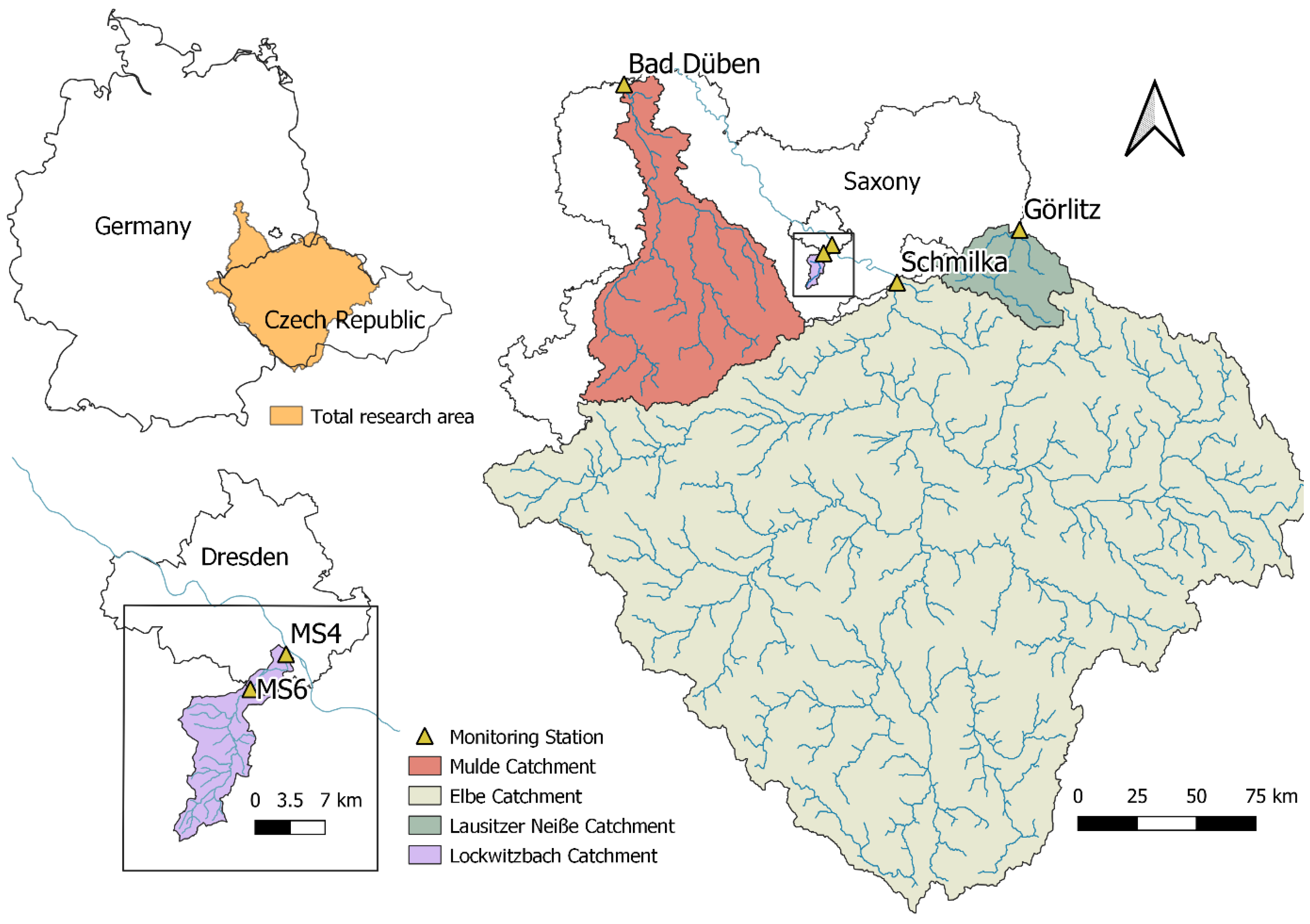
2.1. Catchments and Monitoring Sites

The data evaluated in this study originates from five monitoring stations in Saxony, Germany (Figure 1 and Table 1). The large (sub-) catchments of Elbe (51,387 km2), Mulde (6207 km2), and Neiße (1418 km2) are monitored by the Saxon State Operational Agency for Environment and Agriculture (BfUL), and data was provided by the Saxon State Office for the Environment, Agriculture, and Geology (LfULG). Sensor maintenance and calibration was carried out approximately bi-weekly by BfUL, and data went through a manual correction process. At Lockwitzbach (84 km2), there are two stations operated by the Chair for Urban Water Management of TU, Dresden [32]. The stations are about 6 km apart; one is located before the stream reaches the city of Dresden (MS6, upstream Dresden), the other shortly before the confluence with Elbe (MS4, downstream Dresden). Weekly site visits and bi-weekly sensor calibration were carried out at both monitoring stations, and analyzed data were corrected by the staff of the institute. According to the results of the latest river management plan period, all four waterbodies fail to achieve a good chemical status, particularly due to the exceedance of annual average concentration limits of total-phosphorus, mercury, and polycyclic aromatic hydrocarbons [33].

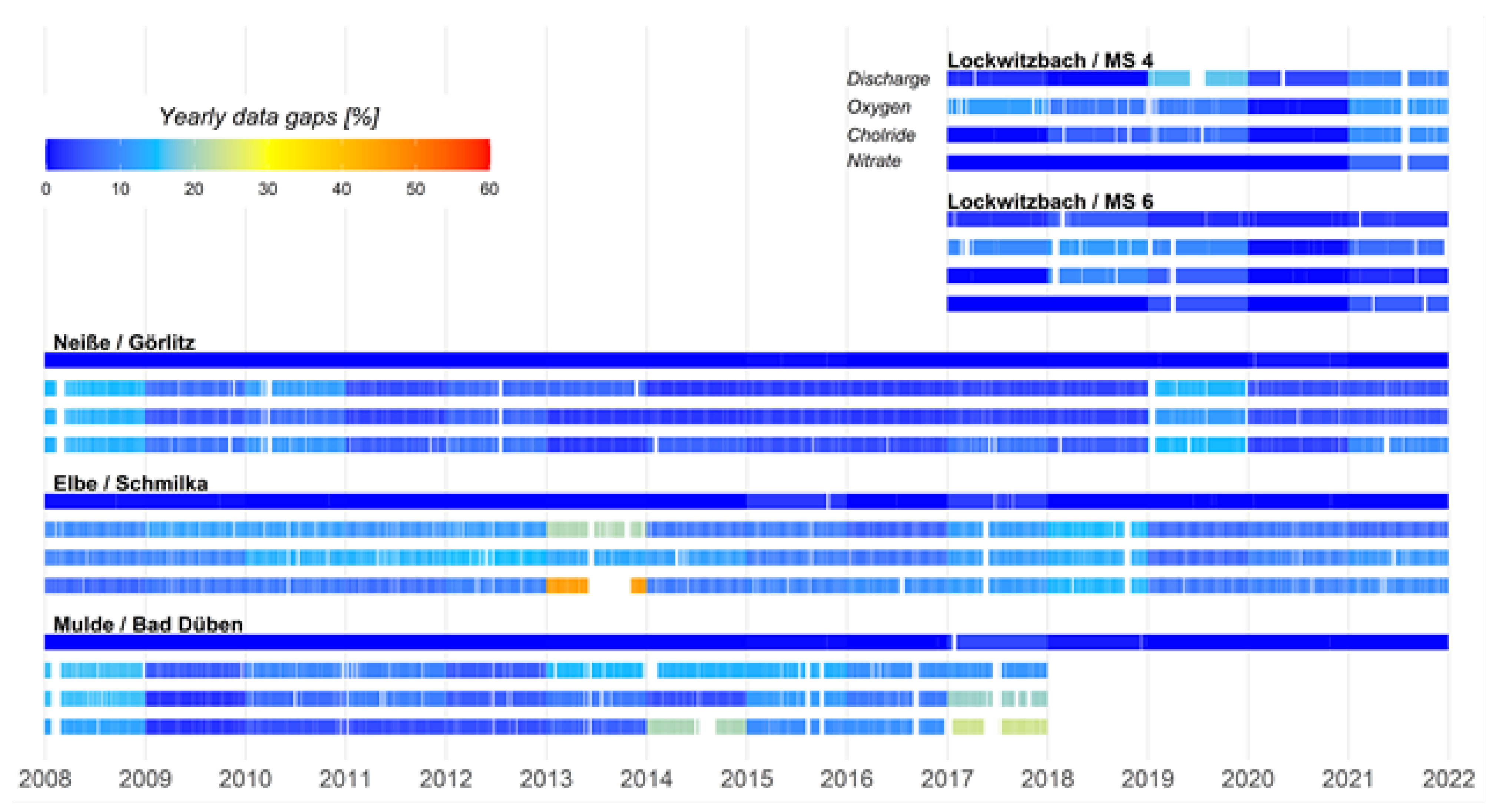
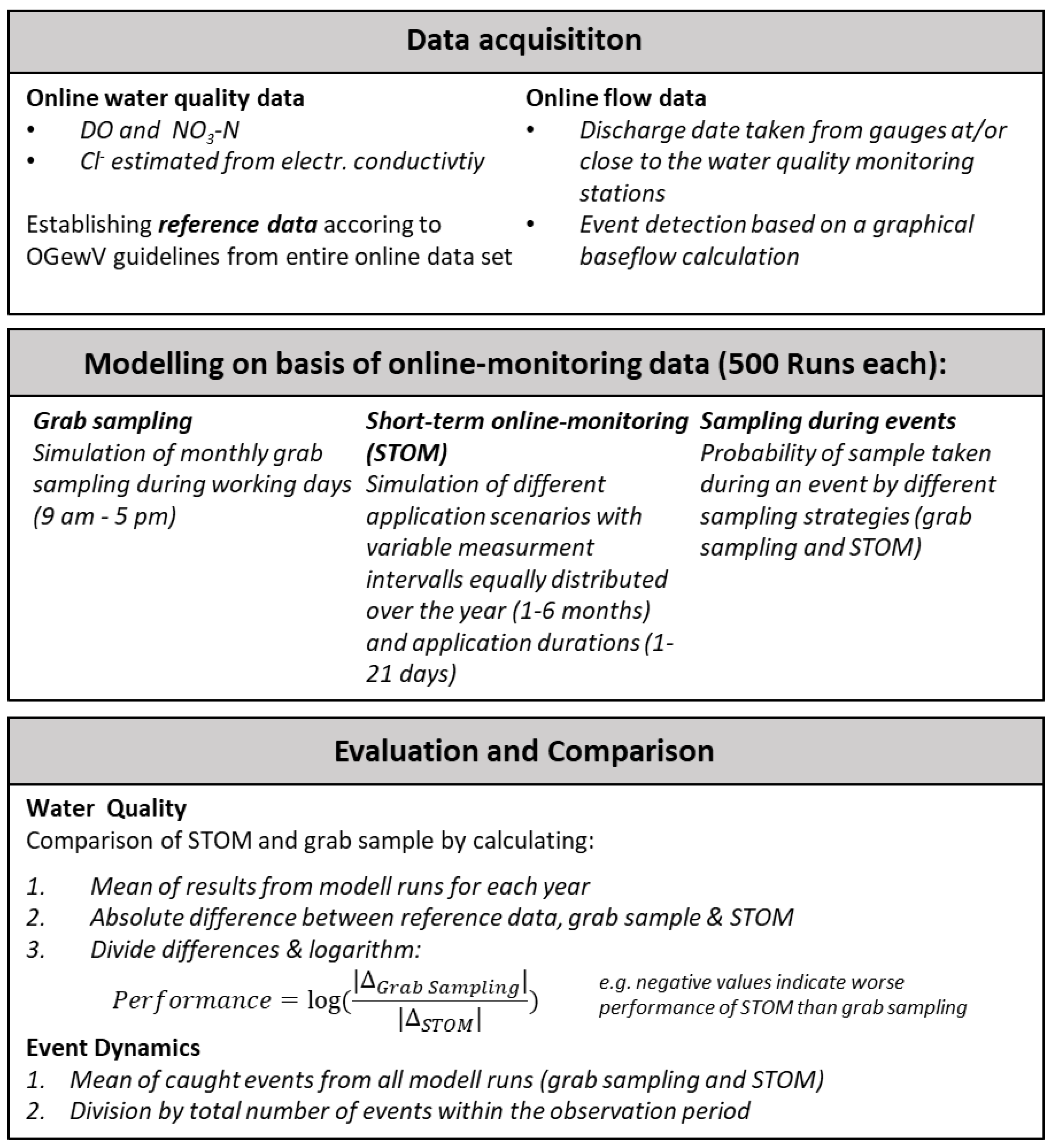
2.2. Water Quality and Discharge Data

The study evaluates the concentrations of nitrate-nitrogen (NO3-N), dissolved oxygen (DO), and chloride (Cl), recorded with a temporal resolution of 10 min. Nitrate-nitrogen was measured by adsorption spectrometry (Nitratax, Hach, Loveland, CO, USA and ColorPlus 3 Nitrat, Sigrist, Karlsruhe, Germany) and dissolved oxygen by luminescence (FDO 700 IQ, WTW, Weilheim, Germany). Chloride concentration was derived by a linear model from grab sample chloride concentration and electric conductivity using an ordinary least squares approach (Supplementary Materials, Figure S10). Electric conductivity was measured by direct current method (TetraCon 700 IQ, WTW, Weilheim, Germany).
At Lockwitzbach, we (Chair of Urban Water Management) measured dissolved oxygen with a LDO sc probe (Hach, Loveland, CO, USA), and nitrate-nitrogen was measured optically (spectro::lyser, s::can, Vienna, Austria) and, furthermore, with an ion-selective probe (ANISE sc, Hach, Loveland, CO, USA), which also records chloride at an interval of 10 min. For NO3-N, we mainly used the optical measurement results from the spectro::lyser and filled the gaps with ANISE sc data. Mean yearly and seasonal concentrations of the five monitoring stations and their standard deviation and diurnal ranges can be found in Table 2.
Discharge data were selected from flow gauges at the respectively shortest distance to the water quality stations. At Elbe, Vereinigte Mulde, and Lausitzer Neiße, the BfUL operates flow gauges not further away than 7 km from the water quality stations. At Lockwitzbach, flow rates were established at the monitoring sites. Monitoring periods of the water quality recordings were 5 years (Lockwitzbach), 10 years (Mulde), and 14 years (Elbe, Neiße). On average, 7% of the three water quality parameters (nitrate-nitrogen, chloride, and dissolved oxygen) were missing every year. The recorded discharge data were more complete, with 2% of data missing per year. Highest gap was found for MS4 in 2019, with 16% of data missing. About 23 million measurement points were evaluated; the length of the datasets, as well as their completeness, are shown in Figure 2.
The importance of the investigated parameters, as well as the thresholds for the classification for a water body, are stated in §5 and §6 OGewV [35], referring to appendices 3, 4, 7, and 8. Dissolved oxygen and chloride are considered as physico-chemical components. These parameters serve as supporting parameters for defining the ecological status of a water body, while the biological and chemical components are the main criteria. Based on the river type, the threshold concentration for the mean annual minimum dissolved oxygen concentration varies between 9 mg/L (Lockwitzbach) and 8 mg/L for all other investigated streams to reach a very good status; for a good status, 8/7 mg/L is required. The annual mean of the chloride concentration needs to be below or equal to 50 mg/L for a very good status and below 200 mg/L for a good status at all river types. The mean annual nitrate concentration threshold is given with 50 mg/L NO3 (11.3 mg/L NO3-N). The parameter is among 46 compounds that are used to define the chemical status. If one of them exceeds the environmental quality standard, the water body fails to achieve a good status.
The “real or reference concentrations” were calculated according to the guidelines of the OGewV, which states different ways to calculate the concentrations for classification, depending on the parameter. The yearly mean value of nitrogen-nitrate is required. Similarly, the arithmetic mean value for chloride should be taken. However, for chloride, a series of three consecutive years can be used for the calculation of a mean value. The same applies for dissolved oxygen, albeit with the mean of a window of three consecutive yearly minimum values. This reduces the effect of outliers on the water quality status. For simplification, we omitted this rule concerning the 3 year window, except for the DO concentrations at Lockwitzbach/MS4, where we observed close to zero DO concentration in 2 years, respectively (2018/2020). In 2018, there was a severe CSO event that led to almost zero DO concentration and lasted for about half an hour. On six days in August 2020, there was almost no discharge in Lockwitzbach, and we observed anoxic conditions during the night.

2.3. Modeling of the Sampling Strategies

To answer the initial research question of how the results of STOM compare to grab sampling, we performed a systematic subsampling of the previously described data. Figure 3 gives a quick overview of the entire modeling process. Results for three sampling strategies were calculated, namely grab sampling, STOM sampling, and event sampling, further described in the next subchapter. All calculations were carried out with R; functions and scripts can be found on github (see credentials) [36].

2.4. Modeling of Grab Sampling

The OGewV requires quarterly to monthly grab samples for determining physico-chemical parameters and monthly sampling for priority compounds of the OGewV, listed in Appendix 8. Based on this, and the information on sampling routine by the LfULG, we decided to randomly sample the time series with a frequency of once a month, on working days and between 9 am and 5 pm. Using these parameters, grab sampling was simulated 500 times, and the rules of the OGewV calculation were applied for these yearly datasets. The mean and the standard deviation of these results was calculated.

2.5. Modeling of Short-Term Online-Monitoring—STOM

In contrast to grab sampling, STOM obtains continuous monitoring data in defined, limited intervals and for limited durations. The duration of the STOM application was selected between 1 and 21 days (the term sensor application duration is used for this dimension in the following). For application intervals, the limits were set from once per month to once every 6 months (the term return interval is used for this dimension in the following). For these time series, we applied the previously explained regulations, according to the OGewV guidelines. The two parameters (application duration and return interval) were varied, and sampling was simulated 500 times. A 6 × 21 matrix was obtained for the means of the model run for every year and parameter at a monitoring station.
To compare STOM and grab sampling strategies, we calculate a performance index, which is defined as the logarithmic quotient of the sampling accuracy of STOM and grab sampling. The sampling accuracy was calculated using the absolute difference between the “real concentration” and the model results of STOM and grab sampling (see the formula in Figure 3). We log transformed the values to indicate whether STOM or grab sampling yielded better results, e.g., negative performance indicates that grab sampling achieves results closer to the “real concentration” than STOM. To identify an unambiguous threshold for the parameter settings that lead to the performance of STOM surpassing that of grab sampling, a model was fitted to the data and used to identify the point where the performance is close to zero (indicating a similar result of STOM and grab sampling). For the model, a linear relation between performance and application duration was identified. For return interval and performance, the values followed a logarithmical trend, regression was carried out using the least square method and yielded a mean coefficient of determination (R2) of 0.9.

2.6. Modeling of Sampling during Events

To find out whether STOM or grab sampling was carried out during a high discharge event, we had to carry out an event selection. Therefore, a base flow time series was calculated by a graphical method, based on the work of Gustard et al. (1992) [37]. Events were subsequentially selected if flow was 10% higher than the calculated baseflow. In general, there are many different approaches to identify base flow (for an overview on base flow calculation e.g., [38]). We used a graphical method for the event selection, since it provides a precise time selection of events.
Gustard et al. (1992) [37] developed his method for daily resolution discharge data. However, we applied it to data with a high temporal resolution (5 and 15 min). Therefore, we varied the window widths used to calculate the daily mean values so that events with a duration below 1 day could also be separated from baseflow. That was of higher importance for smaller catchments, where event durations are considerably shorter than in bigger watersheds, such as Elbe. Hence, depending on the size of the catchment, we used shorter window widths to calculate the mean values: between 4 h and 24 h in hydrological summer and between 12 h and 36 h in hydrological winter, instead of a one-day window. The subsequent procedure is similar to that of Gustard et al. (1992) [37], who calculated the local minima of five-day non-overlapping consecutive periods and identified turning points by restricting increases by gradient filtering with the previously calculated, higher resolved minima-time series. These turning points are connected by linear interpolation; they form a base flow hydrograph. To identify events, the time series was split into hydrological winter and summer. We defined the thresholds of different parameter sets considering: (1) events having a discharge 10% higher than base flow; (2) minimum duration; and (3) the minimum discharge difference between the event minimum and maximum. For the discharge signal, we used the number of samples that were taken during an event and compared this with the total amount of detected events every year.

2.7. Uncertainty of Sampling Strategies

Similarly to the performance comparison, we analyzed the uncertainty of both sampling strategies by their relative standard deviation. The modeling results of both STOM and grab sampling for every station and parameter were used. Therefore, we took the average of the yearly standard deviations divided by the yearly mean concentration. The comparison was carried out by the quotient of the relative standard deviations of STOM and grab sampling. A value greater than 1 indicates that conventional sampling has a smaller standard deviation, whereas a value below 1 indicates the opposite. In a similar way to the previous comparison of the results from STOM grab sampling, a log-linear regression was fitted to identify the turning point where the quotient is below 1.

2.8. Cost Calculation

In order to show how STOM behaves from an economic perspective, we performed a rough cost estimation. As an example, we used the previously analyzed water quality parameters at the five monitoring sites. We met the following assumptions to estimate yearly monitoring costs:
Grab sampling:
  • Grab sampling is assumed to be carried out 12 times per year.
  • €8 per sample for the analysis of NO3-N and Cl; O2 is measured on site with a hand-held device for €642 per year (€4500 over 7 year depreciation period).
  • Driving costs of €4.5 per site and €240 personnel costs per sampling day (8 h with an hourly wage of €30).
STOM:
  • Intervals for STOM vary on the different application scenarios
  • Multi parameter probe (€15,000) with a depreciation period of 7 years (€2143/year). The number of sensors depends on return intervals and duration of sensor application.
  • Driving and personnel costs based on the values of grab sampling but multiplied by two, since the sensor needs to be installed and picked up.

3. Results

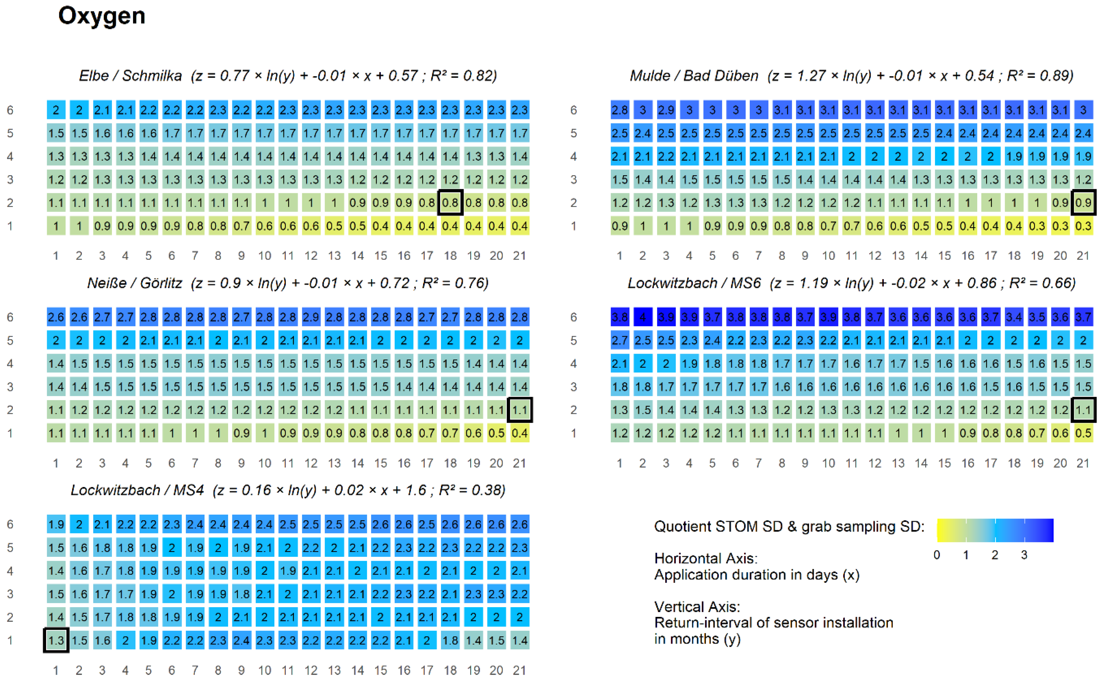
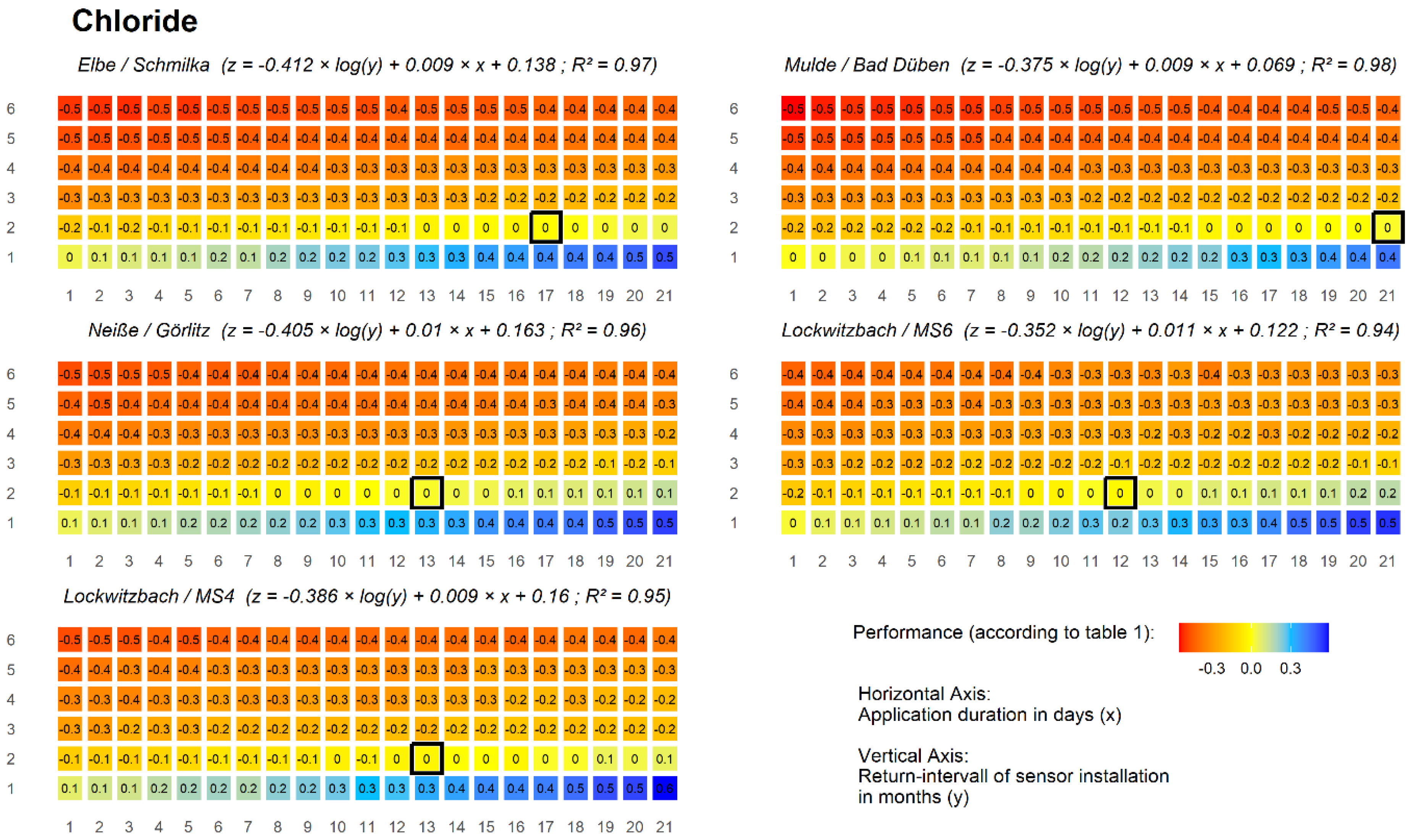
3.1. Water Quality Parameters

For a general overview of the comparison between STOM and grab sampling, the mean of all yearly performances (according to Figure 3) were calculated and concluded as a heat map. Results for single years can be found in the supporting material. The parameters were chosen from the 6 × 21 matrix (1–6 months return interval and 1–21 days of sensor application duration) and selected to favor a lower interval of return over the duration of the sensor application. For example, if a similar performance of zero was achieved for either a 3 month return interval and 20 days of sensor application, or for a 2 month return interval and 2 days of sensor application, the first parameter set was chosen (as a longer application is feasibly easier than a regular installation of the sensor). The predicted intercepts, or break-even points, where STOM becomes more accurate than grab sampling are marked in the following graphs with a black frame. Differences between empirical (the number in the box) and fitted intercepts of the performance index are caused by deviation between the mixed linear regression model and resampling data. The results of the five monitoring stations are sorted by parameter and catchment area.
For nitrogen-nitrate, monthly grab sampling led to a 3.0% mean absolute deviation, or assessment error, from the complete data set. Mean grab sampling errors were similar among all catchments, ranging from 2.5 to 3.5%, with a tendency to be reduced by increasing watershed size.
As Figure 4 shows, STOM outperformed grab sampling at similar duration–interval combinations in all catchments. Return intervals were monthly or bi-monthly, whereas a duration of 1 day sufficed in four out of five catchments. For all catchments, the resampling-based performance yielded similar or better performance with monthly one-day STOM.
The coefficient for STOM sampling duration was extracted from the mixed linear regression model and ranged from 0.007 to 0.01, with the lowest value at Mulde river and the highest at Neiße river, the two intermediate size rivers in the study. This indicates a systematic improvement of the relative STOM performance with increased sampling duration. Notably, the performance improvement is more pronounced at shorter return intervals. The coefficient of log-transformed sampling interval ranged from −0.44 to −0.52, again with Mulde (lowest) and Neiße (highest) defining the range. Hence, for Mulde river, STOM performance appeared more sensitive to return interval, while for Neiße, sampling duration was more decisive.
The results of STOM for single years also did not exceed a return period of 2 months. In 2013, in Neiße, STOM showed the best outcome, indicated by the earliest breakeven point among all stations, with a return interval of 3 months and an application duration of 15 days.
The overall mean values for chloride exhibited similar patterns to nitrogen-nitrate. Monthly grab sampling led to 3.6% mean absolute deviation, or assessment error, from the complete dataset. While the smallest catchment (Lockwitzbach, Neiße) showed the highest mean absolute errors (4.2% and 4.3%), the error margin was reduced towards bigger rivers (to 3.5% at Mulde and 2.0% at Elbe).
For all catchments, a return interval of 2 months provided better performance for STOM than grab sampling. Application durations at the break-even point ranged between 12 to 21 days (Figure 5). Combinations of monthly one-day sampling or bi-monthly 15-day sampling always outperformed grab sampling.
The coefficient for STOM sampling duration ranged from 0.009 to 0.011, with the lowest value at Mulde river and the highest at Lockwitzbach/MS6 river. This indicates a slightly stronger improvement of the relative STOM performance with increasing sampling duration, compared to nitrate results. The coefficient of log-transformed sampling interval ranged from −0.35 at Lockwitzbach/MS6 to −0.41 at Elbe, which corresponds to the smallest and largest catchments in the study. Hence, for chloride sampling, return-interval is more decisive in large than in small catchments, despite larger summer/winter differences at Lockwitzbach (compare to Table 2).
STOM showed better performance than to grab sampling among all stations and all years, with a return interval of 3 months and 17 days in 2014 at the monitoring station in Görlitz (Neiße) and at MS6 (2018). However, the worst scenarios were found at Elbe/Schmilka for several years, with a similar performance to nitrogen-nitrate (1 month return interval and 1 day of application) in 2014, 2015, 2016, 2017, 2018, and 2020 and in Mulde/Bad Düben in 2009, 2013, 2014, 2016, and 2017.
Monthly grab sampling led to 80.4% mean absolute deviation, or assessment error, from the complete data set. Lockwitzbach showed both the highest and smallest mean absolute errors (MS6: 20% & 246%). No effect of catchment size on the error could be identified. Neiße in Görlitz showed an error of 42.6%, Elbe in Schmilka 31.2%, and at Mulde in Bad Düben 61.8%. DO sampling performance underlines the potential of STOM for all catchments; a return-interval of half a year was sufficient, with an application duration of between 1 and 19 days, depending on the stream, to be as good as monthly grab sampling (Figure 6). In all cases, a STOM regime of 3-monthly sampling during 1 day or 5-monthly sampling during 12 days outperforms monthly grab sampling.
The coefficient for STOM sampling duration ranged from 0.014 to 0.022, with the lowest value at Lockwitzbach/MS 6 and very similar values at the larger water bodies. Hence, of all three water constituents, dissolved oxygen sampling accuracy benefits most from longer STOM sampling duration. The higher coefficients at both Lockwitzbach stations coincide with more pronounced day/night differences there. The coefficients of log-transformed sampling interval ranged from −0.21 at Lockwitzbach/MS4 to −0.48 at Elbe, suggesting that oxygen sampling at the larger rivers benefits more from a reduced return-interval than sampling at the smaller stream. For several years, the rarest option (6 month return interval and 1 day of monitoring) were reached at Mulde/Bad Düben (2018) and MS4 (2018, 2019, and 2020). For Elbe/Schmilka and Neiße/Görlitz, 5 month return intervals and 18/21 days of sensor application produced the worst performances in 2009 and 2012, respectively. According to the OGewV, the yearly minimum DO concentrations, or the mean of a maximum of three consecutive yearly minima, need to be selected for the classification. Results from STOM with frequent return intervals and long application duration frequently detected the “real” yearly minimum value, according to the OGewV regulation. These values were omitted for the calculation of the presented mean values as well as in the uncertainty assessment, since this case is not defined because of a division by zero (ΔSTOM = 0, division by zero, see Figure 3).

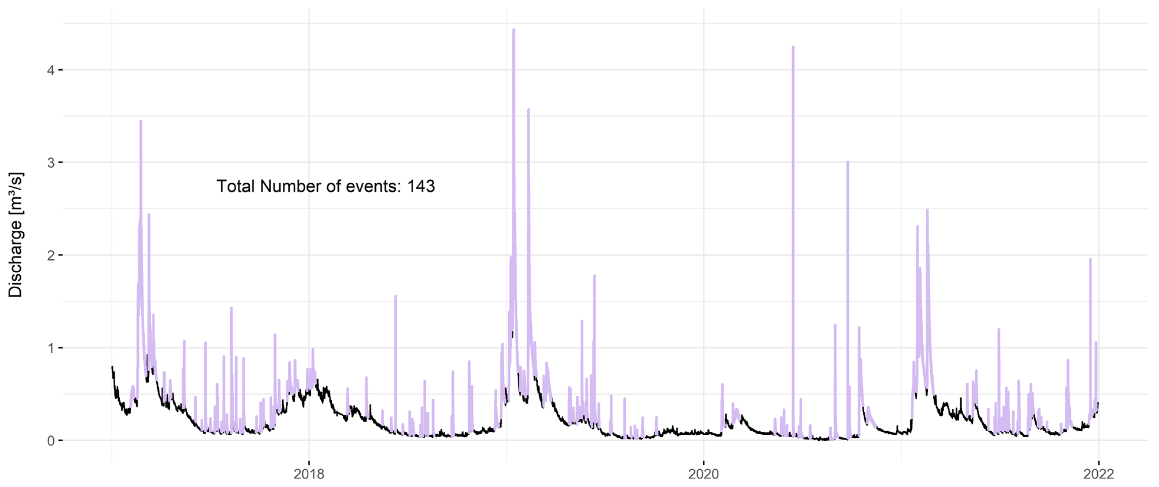
3.2. Sampling during Events

On average, the Lockwitzbach catchment shows the highest yearly number of events and as well as the highest standard deviation between the years (28.6 ± 8 events at MS4, 27.8 ± 9 at MS6, see Figure 7), followed by Neiße and Mulde (18.2 ± 7 and 10 ± 4). A mean of 7.4 ± 2 events per year was calculated for Elbe. Summarizing the duration of all events per year at Lockwitzbach resulted in 81.4 ± 19 and 83.6 ± 22 (MS6/MS4) days on average. At Elbe and Mulde, these values were higher, with 109.3 ± 41 and 105.8 ± 44 days. Neiße had the shortest event duration of 70 ± 32 days per annum. The results of the simulation show that taking a grab sample once per month during an event is very unlikely; for all monitoring stations, an average probability of 0.3% was calculated (Elbe: 0.52%, Mulde: 0.51%, Neiße: 0.21%, and Lockwitzbach MS6/MS4: 0.03/0.1%).
A relation between the yearly event duration, or the number of events per year, and an increase in probability of an event-grab sampling could not be found. Contrary to that, the results of the simulation using STOM show that the probability of taking a sample during an event is significantly higher (Figure 8). Under the most labor-intensive setting (monitoring every month for 21 days), about 52 ± 2% at MS6 to 92 ± 13% at Elbe (long lasting events at Elbe lead to multiple detections during one event) yearly events were caught over all monitored years (75 ± 13% Mulde, 55 ± 7% at Neiße, and 53 ± 4% at MS4).

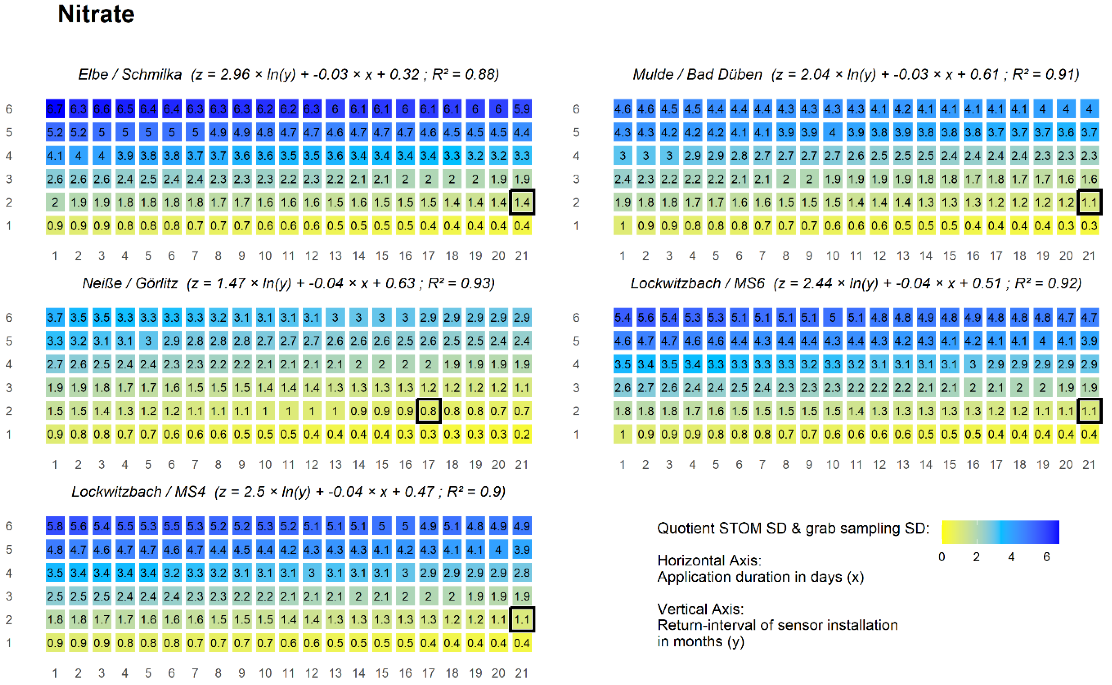
3.3. Uncertainty of the Sampling Strategies

The application duration and the return interval for the break-even point of the quotients of the relative standard deviation do not coincide with the previously gained results from the performance comparison (Figure 9, Figure 10 and Figure 11). In general, a shorter return interval and a longer application duration decrease the relative standard deviation in all cases. Nitrate-nitrogen reaches a smaller quotient of standard deviation earlier at all monitoring stations (than in the performance comparison), and chloride slightly later. Dissolved oxygen, which had a high performance, requires shorter measurement intervals to reach an equal standard deviation to grab sampling.

3.4. Cost Calculation

According to the chosen assumptions, one year of grab sampling costs about €3673 for the three investigated parameters at the five monitoring sites. Costs for STOM vary between €14,439 and €3121, the highest prices occurring with the highest return intervals and the longest sensor application durations. Particularly for long application durations, it would be necessary to fit more multi-parameter sensors to the monitoring framework, leading to exponentially rising costs. A matrix with the yearly monitoring costs for STOM can be found in the Supplementary Materials (Table S2).

4. Discussion

4.1. Estimation of Chloride Concentration

We were using a linear regression model to calculate the chloride concentration from the electrical conductivity. The obtained regression equations revealed similar parameters (Supplementary Materials: Figure S10) between the catchments and were in accordance with values reported in the literature [39,40]. Other studies found that the linear relation between electrical conductivity and chloride is different for lower concentrations due to a change in the composition of solutes and their effect on the electrical conductivity of water. To overcome this issue, Perera et al. (2009) [41] used a second linear regression for this specific value range. Our dataset did not show evidence of such a breaking point, most probably because of the lack of grab sample data with low conductivity/chloride concentrations.

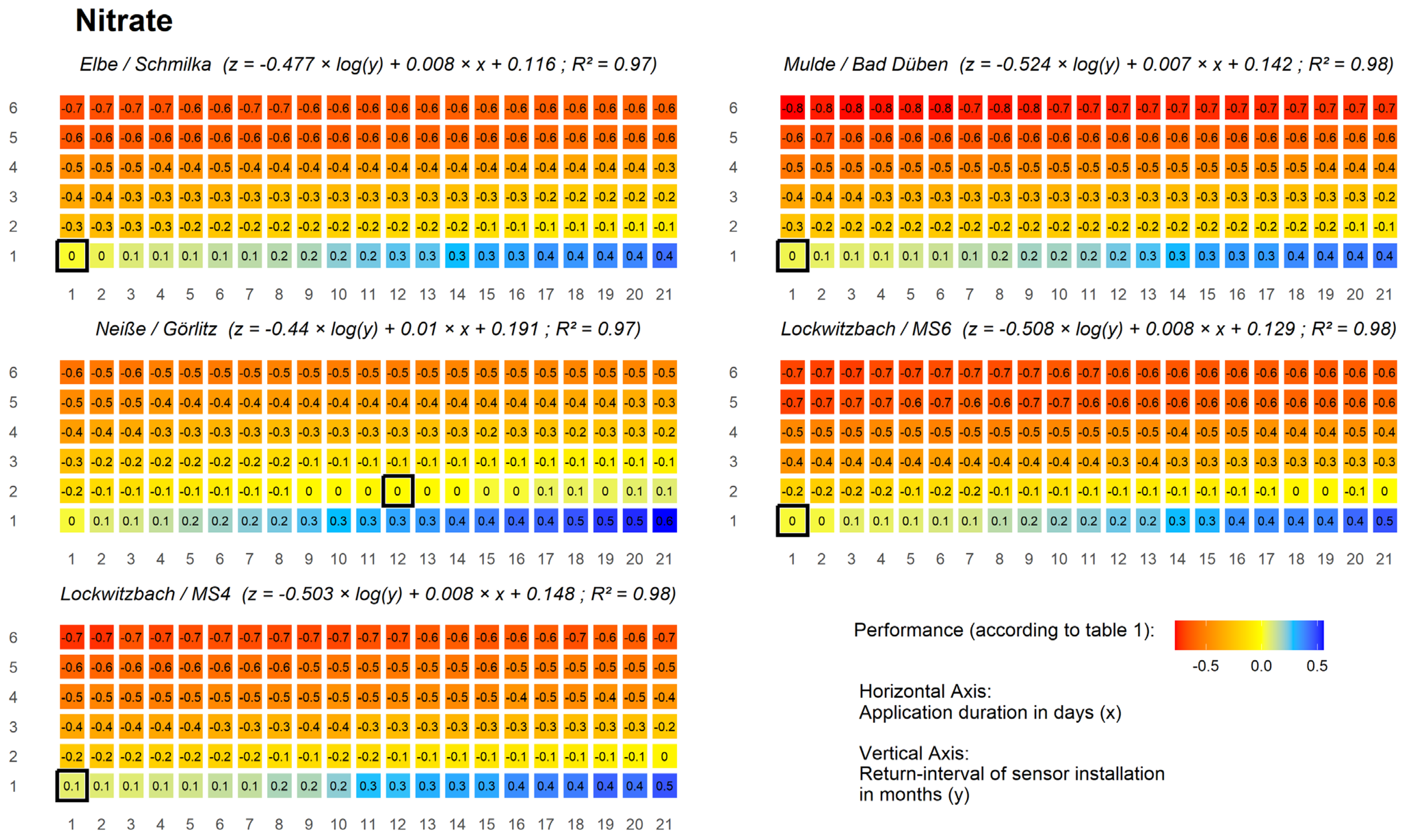
4.2. Performance of STOM in Comparison to Grab Sampling

We defined that grab sampling happens during workdays from 9 a.m. to 5 p.m. to be close to regular working hours. Increasing this time frame further by including the weekend did not lead to significant improvements; on average, the break-even point between grab sampling and STOM was extended by half a day of sensor application. If grab sampling took place during the whole day (24 h), nitrogen-nitrate and chloride would not show significant improvements, but the monitoring of DO would be considerably better. This resulted in a prolongation of the break-even point with STOM by an average amount of 5 days at all monitoring stations, ranging from 2 days in Schmilka to 9 days at MS4. The graphs similar to Figure 4, Figure 5 and Figure 6 for those sites can be found in the Supplementary Materials.
Our results revealed that catchment size does not affect the performance of STOM and grab sampling differently (according to Figure 3); for dissolved oxygen only, a slight tendency for a better performance at small catchments can be suspected. The interval of application (e.g., if the sensor is placed once every month or every second month) has a significantly higher influence on the performance of STOM than the duration of the sensor application. The relation between an increase in performance and the duration of the sensor application can be well represented with a linear function. In contrast, the relation between the performance and the return interval follows a logarithmical trend, indicating a nonlinear performance-improvement with a shorter return interval. These findings are underlined by the factors of the regression functions (see Figure 4, Figure 5 and Figure 6), which are consistently higher for the return interval. Probably, longer return intervals do not represent seasonal and inter-seasonal changes to rivers sufficiently and cannot be compensated by longer sensor application time. The variability of the relative standard deviation seems to be independent of the catchment size and water quality parameters. Performance is more variable between parameters and watersheds, mainly because we calculated the mean of the yearly value durations, which had a high variability as well as a small sample size of 14, 10, and 5 years (details: Figure 2).
To follow up on our initial research question, we found out that the analyzed parameters showed noticeable variations among each other. Particularly for DO, STOM leads to a considerable improvement of monitoring accuracy. The diurnal pattern of the dissolved oxygen concentration, controlled by photosynthesis and respiration in the aquatic ecosystem, appears to be well recorded by STOM. Unlike for nitrate and chloride, the OGewV defines the minimum DO concentration as a threshold, which is also more likely to be caught during longer application periods of continuous monitoring than by a grab sample. Other researchers have identified this previously, such as Halliday et al. (2015) [14], who recommend the establishment of specific sampling time windows for certain WFD parameters, or the use of online sensors, stating that this had already been carried out at a number of sites in England [42].
The small difference between grab sampling and STOM for nitrogen-nitrate and chloride can be explained by the comparably low variability of both parameters, which are mainly affected by seasonal changes or by dilution during rain events. Fluctuations in nitrate concentration and the effect of rainfall characteristics on this were studied by Winter et al. (2022) [43] on six sub-catchments of the Bode River. They found strong drivers in event magnitude and seasonality that are controlling the relevant flow paths of nitrate within the land-to-stream connection. Even though some publications mention that diurnal patterns were detected for nitrate, our dataset did not show those trends, or only marginal amplitudes were visible [4,44,45]. Vilmin et al. (2018) [12] concluded that with a grab sampling frequency of 25 days per year, a good representation of the mean nitrate concentration of the Seine in Paris can be achieved. Bieroza et al. (2014) [4] stated that a weekly and monthly sampling was adequate for their investigated agricultural catchment in Sweden.
Studies on the importance of sampling frequency for chloride concentration assessment are rare. Harmeson and Barcelona (1981) [46] mention that the average deviation of monthly samples was found to be acceptable for chloride in Illinois’ watersheds. Generally, several papers reported linkages between the chloride concentration and discharge, e.g., a dilution of chloride by increased streamflow and vice versa [47]. Particularly from the northern hemisphere, there are manifold studies focusing on the additional input of salt during the winter months by road salt applications [40,48,49]. By using a yearly mean value for classification instead a maximum value, the OGewV rather neglects these spikes from road salt application. Reports in the literature warn about several adverse effects of increasing salinization in water bodies [50,51,52]. Only at Lockwitzbach were peaks above 200 mg/L for some hours measured during winter, and these are below acute toxicity, as defined by CEQG (2011) or US EPA (1988) [53,54]).
The two monitoring stations at Lockwitzbach (MS6 & MS4) also allow us to investigate the influence of sampling location on classification in small streams. For chloride, there is a small difference between the monitoring stations, with 3% difference on average over all years relative to the mean concentration at MS6. Nitrate shows a slight reduction of 9% between the stations, probably caused by increased nitrate uptake and denitrification during the summer months. If a mean value would also be used as the rule for oxygen according to OGewV, as it is for nitrate and chloride, there would be hardly any difference cognizable between the two stations (0.5%). However, the rules for dissolved oxygen calculation are set using the yearly minima for classification, leading to a mean reduction of 63% between the two monitoring stations. The decrease between the two monitoring stations arises as a result of pronounced day patterns of dissolved oxygen at MS4, reaching considerably lower concentrations in the summer nights. Changes in the catchment characteristics lead to the following results: the stream flows from a rather rural area (MS6) through the city of Dresden. The station MS4 is located at the outlet of this urban section shortly before the confluence with Elbe river. Within this urban section, the water body lacks natural shade from trees and bushes. The cross-section is comparably broad, with shallow water levels that expose a high surface area to sunlight. According to the official information provided by LfULG, one sampling location is used for the chemical classification of Lockwitzbach (https://www.umwelt.sachsen.de/datenportal-ida-4626.html, Accessed on 29 July 2023). This is located close to MS6 and would not produce these large differences. Choosing sampling locations based on an analysis of catchment land use would help to overcome such underestimations and reveal the potential for improved measurement in the watershed.
Considering the very limited number of parameters that we can measured online with affordable probes, STOM would not be able to replace grab sampling completely. However, we consider that STOM can be smartly combined with grab sampling to extend the value of the gathered water quality information and to deepen our understanding of the hydrological and chemical dynamics of rivers [55,56,57]. Article 7 of the WFD distinguishes between the monitoring objectives of surveillance monitoring, operational monitoring, and investigative monitoring. Surveillance monitoring should identify the status of the water body, recognize long-term changes, and provide guidance for future monitoring campaigns. Operational monitoring surveils waterbodies which fail or are at risk of failing their environmental objective and verifies the effectiveness of measures. Investigative monitoring is intended to identify the reason for unknown degradations of the water quality, e.g., during accidents leading to leakage or spills of pollutants. The application of STOM outside of operational monitoring seems promising. It can be used for investigative monitoring, which is usually carried out less frequently but with more effort [18]. Among other examples, the federal state of Saarland in Germany has been successfully carrying out investigative monitoring for several years by using online monitoring over a certain time span for “at-risk” water bodies to identify and evaluate the contributions of point sources and diffuse pollution, crosscheck the efficiency of measures to improve ecosystem quality, and capture the eutrophication state of a water body (www.gewaesser-monitoring.de/en/ (accessed on 13 March 2024), [58,59]).

4.3. STOM and Event Sampling

Catchment size seems to have an effect on the standard deviation of the number of yearly events, showing higher a variability in the number of yearly events at smaller catchments. Unlike the investigated water quality parameters, there is a clear tendency for bigger catchments to show a higher probability of catching a sample during an event using STOM sampling. Looking at the regression equations for event sampling, it becomes obvious that the application duration has a higher importance for event monitoring, while for water quality parameters, the return interval had a more pronounced impact.
The simulation showed that there is no clear positive correlation at all catchments between the number of events sampled by STOM and their duration or the number of yearly events. Even under long exposure and regular installation of sensors, only Neiße showed a correlation for both and Elbe only for the event duration. As already mentioned in the previous chapter, datasets for Lockwitzbach are considerably shorter than the ones for Elbe, Vereinigte Mulde, and Lausitzer Neiße, and are not suitable for a meaningful statistical analysis.
The German Working Group of the Federal States and the Government on Water Issues (ref. [1]) recommends 12 samples per year for compounds that show a strong variance in their concentration or that are introduced on the basis of special occasions or sampling during the period of usage. The results of the simulated grab sampling strategies for event monitoring shows that it is not possible to reliably monitor pollutants that are mobilized during rain events by taking a sample once per month. According to Rügner et al. (2019), the total pollutant concentration is the sum of the dissolved and particle-associated fractions. The particle-associated fraction is the product of total suspended sediment (TSS) and the concentration of the compound on the suspended particle [60]. Often, the logKOW (octanol/water partitioning coefficient, a measure for hydrophobicity) is used for estimating the sorption coefficients of compounds to soil or sediments [61]. There are 46 compounds that are used to classify the chemical status of a waterbody in Appendix 8 of the OGewV by using a maximum mean concentration. For 30 out of those 46 compounds, a maximum allowable concentration is assigned, which is not allowed to be exceeded in any sample taken. A literature review on the logKOW values showed that only nitrate is highly soluble in water. The other compounds have higher values and are more likely to be attached to particles. Since these relevant compounds are supposed to be measured in the unfiltered sample—except for the heavy metals: cadmium, lead, mercury, and nickel—high solid concentrations during rain events are of most ecological concern according to the chemical classification of OGewV. This makes high flow periods highly important, since a considerable amount of TSS is mobilized together with particle bound pollutants during, and particularly at the beginning of, events (chemodynamic transport or first flush phenomena [62]). Their environmental concentration is highly likely to be underestimated under the current monitoring strategy. Furthermore, if most of the mobilized sediments are transported at the beginning of an event, the probability for catching representative grab samples becomes even smaller. Only special event sampling programs using automated samplers or sediment collectors would improve the accuracy of the standard monitoring program. However, to operate and maintain such an extended program for all streams is unrealistic for many reasons—mainly the amount of personnel required for handling samplers and the capacity required for the analysis of samples [63]. Automated sensors can overcome those drawbacks to a certain extent. However, they require extensive maintenance. Comparing STOM and passive sampling for the estimation of mean concentrations might provide insights about the potential of using less resource-intensive sampling approaches. Since STOM can improve monitoring on event mobilized compounds, further parameters that can be measured with online sensors are promising, such as turbidity or SAK254. These parameters can also be used as proxies for further compounds. However, for several WFD-relevant parameters, whilst technologies are available they are still far away from field application [64,65,66,67], and a faster development of online-sensors would be desirable [17].

4.4. STOM for Modeling

Recent publications show the benefit of using different river models for the status assessment of water bodies, parameters, sampling frequency, and location [12,68,69,70]. We want to emphasize the value of data generated by STOM for further improving the model quality, particularly in the calibration and validation process. In other studies, such as in a flashy Finnish watershed, for example [7], the benefits have been shown of model predictions for sediment and nutrient loads that use high-frequency data and more frequent sampling as a calibration source for several parameters in order to improve KGE. Nafees Ahmad et al. (2011) [71] showed that monthly samples lead to a considerable underestimation of SWAT model results for sediment and nitrogen loads during high precipitation events in comparison with a high resolved time series. However, other studies found that nitrate measurement frequency (daily to fortnightly) do not influence the total uncertainty of nitrate predictions, since the combination of model structural errors and measurement errors were much higher when compared to parametric prediction uncertainty [69].

4.5. Cost Calculation

According to our calculations for sampling, personnel, and travelling expenses, we found that STOM is cheaper than grab sampling after a return interval of 4 months, irrespective of the application duration. STOM costs are mainly affected by the rising costs of additional sensors, which are mostly required for frequent and long-lasting monitoring campaigns. However, this is an example with simple calculations intended to demonstrate the related costs for both approaches. Conventional sampling regimes consist of a higher number of sampling sites and analytes, leading to a more complex calculation of personnel and travel costs. The grab sampling regime for operation monitoring in Saxony observes about 2240 monitoring sites, and the analysis covers about 420 compounds (120 industrial chemicals, 190 agricultural chemical or pesticides, 80 pharmaceuticals, and 30 metals [33]).

5. Conclusions

After comparing the simulated STOM and grab sampling strategies, our results showed how STOM would fundamentally improve the current approach for monitoring parameters with a pronounced diurnal pattern (such as DO), particularly when maximum and minimum concentrations are requested by regulations or laws. However, for chloride and nitrogen-nitrate, because of their low variability and the usage of mean concentrations for the assessment by the OGewV, we did not see big improvements compared to a monthly grab sampling regime. Taking discharge and high discharge events as a surrogate signal to analyze event-mobilized pollutants, the STOM sampling strategy would increase the probability of capturing pollution spikes by several orders of magnitude. We found evidence that these results are dependent on the catchment size, in contrast to the performance comparison of the three water quality parameters. Taking into consideration the fact that grab sampling fails at monitoring event-mobilized pollutants, it becomes obvious that sampling strategies need to be adapted. Efforts should be made to implement new technologies and approaches as future standard tools for river monitoring to close this gap. In this context, we proposed STOM as an alternative, showing its potential to analyze the chemical and ecological status of a surface water body. The research on the Lockwitzbach catchment, including the analysis of two monitoring points upstream and downstream of an urban area, shows the challenges of monitoring small streams and assessing their ecological quality correctly. In order to further evaluate the benefits of STOM, future studies might consider selecting other proxy-parameters that can be easily measured with a high temporal resolution.

Supplementary Materials

The following supporting information can be downloaded at: https://www.mdpi.com/article/10.3390/w16060889/s1, Figure S1: Performance between STOM and grab sampling at weekend and 9 a.m. to 5 p.m. for nitrogen-nitrate, Figure S2: Performance between STOM and grab sampling at weekend and 9 am to 5 pm for chloride, Figure S3: Performance between STOM and grab sampling at weekend and 9 am to 5 pm for dissolved oxygen, Figure S4: Performance between STOM and Grab sampling during the whole day (0–24 h) for nitrate nitrogen, Figure S5: Performance between STOM and Grab sampling during the whole day (0–24 h) for chloride, Figure S6: Performance between STOM and Grab sampling during the whole day (0–24 h) for dissolved oxygen, Figure S7: Difference between STOM concentration and real concentration for nitrogen-nitrate, Figure S8: Difference between STOM concentration and real concentration for chloride, Figure S9: Difference between STOM concentration and real concentration for oxygen, Figure S10: Linear relation between electrical conductivity and chloride concentration at Mule/Bad Düben, Lausitzer Neiße/Görlitz and Elbe/Schmilka. Shaded area: 95%-confidence interval, dashed lines: Prediction interval; Table S1: Result of 500 simulation runs of grab sampling according to OGewV rules with standard deviation. Sampling frequency were varied between once to every month to two times per year, Table S2: Monitoring costs for STOM in Euro per year

Author Contributions

Conceptualization, J.B.; methodology, J.B. and X.C.; software J.B. and X.C.; validation, J.B. and B.H.; formal analysis, J.B.; investigation, J.B.; resources, J.B.; data curation, J.B. and X.C.; writing—original draft preparation, J.B.; writing—review and editing, J.B. and B.H.; visualization, J.B.; supervision, B.H. and P.K.; project administration, J.B. and B.H.; funding acquisition, P.K. All authors have read and agreed to the published version of the manuscript.

Funding

This research was funded by Helmholz-Wasser Netzwerk, Teilprojekt Urbanes Wasserressourcenmanagement and by the DFG founded project Urban Resistom, grant number KR 2337/17-1.

Data Availability Statement

The discharge datasets used in the present study are publicly available at the Saxonian State Agency for the Environment, Agriculture and Geology (SLULG): https://www.umwelt.sachsen.de/umwelt/infosysteme/hwims/portal/web/download-von-messwerten (accessed on 13 March 2024). Data from Lockwtizbach can be requested from the author. Scripts for the STOM approach and the graphics are available on github: https://github.com/Jakobbenisch/STOM (accessed on 13 March 2024).

Acknowledgments

We would like to thank the Helmholtz-Centre for Environmental Research for funding personnel and monitoring at Lockwitzbach. Further thanks to Reinhard Pohl, Susanne Heise, and Sascha Goldstein from BfUL for sharing data and operating and maintaining the monitoring stations at Schmilka, Bad Düben, and Görlitz. Special thanks for supporting the maintenance of the Lockwitzbach monitoring network go to Robin Mayer, Stephan Becker and Marvin Dropp. Thanks also for the support by the Helmholtz International Research School on Trajectories towards water security (TRACER), which contributed to the development framework.

Conflicts of Interest

Author Xin Chang is now employed by the company Beijing Insights Value Technology Co., Ltd. At the time of contribution, she was a master’s student at TU Dresden. The remaining authors declare that the research was conducted in the absence of any commercial or financial relationships that could be construed as a potential conflicts of interest.

References

  1. LAWA-Ausschuss Oberirdische Gewässer und Küstengewässer; Obmann. Rahmenkonzeption Zur Aufstellung von Monitoringprogrammen und Zur Bewertung des Zustands von Oberflächengewässern; LAWA: Potsdam, Germany, 2021. [Google Scholar]
  2. Hanke, G.; Lepom, P.; Quevauviller, P.; Allan, J.; Batty, J.; Bignert, A.; Borga, K.; Boutrup, S.; Brown, B.; Carere, M. Guidance Document No. 19 Guidance on Surface Water Chemical Monitoring under the Water Framework Directive. 2009. Available online: https://op.europa.eu/en/publication-detail/-/publication/91d313f0-2cc7-4874-b101-a7dba97401b0 (accessed on 13 March 2024).
  3. WFD-CIS. Working Group 2.7 Monitoring, Guidance Document No. 7. Monitoring under the Water Framework Directive; European Communities: Luxembourg, 2003. [Google Scholar]
  4. Bieroza, M.Z.; Heathwaite, A.L.; Mullinger, N.J.; Keenan, P.O. Understanding Nutrient Biogeochemistry in Agricultural Catchments: The Challenge of Appropriate Monitoring Frequencies. Environ. Sci. Process. Impacts 2014, 16, 1676–1691. [Google Scholar] [CrossRef] [PubMed]
  5. Elwan, A.; Singh, R.; Patterson, M.; Roygard, J.; Horne, D.; Clothier, B.; Jones, G. Influence of Sampling Frequency and Load Calculation Methods on Quantification of Annual River Nutrient and Suspended Solids Loads. Environ. Monit. Assess. 2018, 190, 78. [Google Scholar] [CrossRef] [PubMed]
  6. Pace, S.; Hood, J.M.; Raymond, H.; Moneymaker, B.; Lyon, S.W. High-Frequency Monitoring to Estimate Loads and Identify Nutrient Transport Dynamics in the Little Auglaize River, Ohio. Sustainability 2022, 14, 16848. [Google Scholar] [CrossRef]
  7. Piniewski, M.; Marcinkowski, P.; Koskiaho, J.; Tattari, S. The Effect of Sampling Frequency and Strategy on Water Quality Modelling Driven by High-Frequency Monitoring Data in a Boreal Catchment. J. Hydrol. 2019, 579, 124186. [Google Scholar] [CrossRef]
  8. Robertson, D.M.; Roerish, E.D. Influence of Various Water Quality Sampling Strategies on Load Estimates for Small Streams. Water Resour. Res. 1999, 35, 3747–3759. [Google Scholar] [CrossRef]
  9. Wang, J.; Bouchez, J.; Dolant, A.; Floury, P.; Stumpf, A.J.; Bauer, E.; Keefer, L.; Gaillardet, J.; Kumar, P.; Druhan, J.L. Sampling Frequency, Load Estimation and the Disproportionate Effect of Storms on Solute Mass Flux in Rivers. Sci. Total Environ. 2023, 906, 167379. [Google Scholar] [CrossRef] [PubMed]
  10. Carstensen, J. Statistical Principles for Ecological Status Classification of Water Framework Directive Monitoring Data. Mar. Pollut. Bull. 2007, 55, 3–15. [Google Scholar] [CrossRef] [PubMed]
  11. Naddeo, V.; Scannapieco, D.; Zarra, T.; Belgiorno, V. River Water Quality Assessment: Implementation of Non-Parametric Tests for Sampling Frequency Optimization. Land Use Policy 2013, 30, 197–205. [Google Scholar] [CrossRef]
  12. Vilmin, L.; Flipo, N.; Escoffier, N.; Groleau, A. Estimation of the Water Quality of a Large Urbanized River as Defined by the European WFD: What Is the Optimal Sampling Frequency? Environ. Sci. Pollut. Res. 2018, 25, 23485–23501. [Google Scholar] [CrossRef]
  13. László, B.; Szilágyi, F.; Szilágyi, E.; Heltai, G.; Licskó, I. Implementation of the EU Water Framework Directive in Monitoring of Small Water Bodies in Hungary, I. Establishment of Surveillance Monitoring System for Physical and Chemical Characteristics for Small Mountain Watercourses. Microchem. J. 2007, 85, 65–71. [Google Scholar] [CrossRef]
  14. Halliday, S.J.; Skeffington, R.A.; Wade, A.J.; Bowes, M.J.; Gozzard, E.; Newman, J.R.; Loewenthal, M.; Palmer-Felgate, E.J.; Jarvie, H.P. High-frequency Water Quality Monitoring in an Urban Catchment: Hydrochemical Dynamics, Primary Production and Implications for the Water Framework Directive. Hydrol. Process. 2015, 29, 3388–3407. [Google Scholar] [CrossRef]
  15. Skeffington, R.A.; Halliday, S.J.; Wade, A.J.; Bowes, M.J.; Loewenthal, M. Using High-Frequency Water Quality Data to Assess Sampling Strategies for the EU Water Framework Directive. Hydrol. Earth Syst. Sci. 2015, 19, 2491–2504. [Google Scholar] [CrossRef]
  16. Capodaglio, A.G.; Callegari, A. Online Monitoring Technologies for Drinking Water Systems Security. In Risk Management of Water Supply and Sanitation Systems; Springer: Berlin/Heidelberg, Germany, 2009; pp. 153–179. [Google Scholar]
  17. Allan, I.J.; Vrana, B.; Greenwood, R.; Mills, G.A.; Knutsson, J.; Holmberg, A.; Guigues, N.; Fouillac, A.-M.; Laschi, S. Strategic Monitoring for the European Water Framework Directive. TrAC Trends Anal. Chem. 2006, 25, 704–715. [Google Scholar] [CrossRef]
  18. Brack, W.; Dulio, V.; Ågerstrand, M.; Allan, I.; Altenburger, R.; Brinkmann, M.; Bunke, D.; Burgess, R.M.; Cousins, I.; Escher, B.I. Towards the Review of the European Union Water Framework Management of Chemical Contamination in European Surface Water Resources. Sci. Total Environ. 2017, 576, 720–737. [Google Scholar] [CrossRef] [PubMed]
  19. Carvalho, L.; Mackay, E.B.; Cardoso, A.C.; Baattrup-Pedersen, A.; Birk, S.; Blackstock, K.L.; Borics, G.; Borja, A.; Feld, C.K.; Ferreira, M.T.; et al. Protecting and Restoring Europe’s Waters: An Analysis of the Future Development Needs of the Water Framework Directive. Sci. Total Environ. 2019, 658, 1228–1238. [Google Scholar] [CrossRef] [PubMed]
  20. Hering, D.; Borja, A.; Carstensen, J.; Carvalho, L.; Elliott, M.; Feld, C.K.; Heiskanen, A.-S.; Johnson, R.K.; Moe, J.; Pont, D. The European Water Framework Directive at the Age of 10: A Critical Review of the Achievements with Recommendations for the Future. Sci. Total Environ. 2010, 408, 4007–4019. [Google Scholar] [CrossRef] [PubMed]
  21. Halliday, S.J.; Wade, A.J.; Skeffington, R.A.; Neal, C.; Reynolds, B.; Rowland, P.; Neal, M.; Norris, D. An Analysis of Long-Term Trends, Seasonality and Short-Term Dynamics in Water Quality Data from Plynlimon, Wales. Sci. Total Environ. 2012, 434, 186–200. [Google Scholar] [CrossRef] [PubMed]
  22. Minaudo, C.; Meybeck, M.; Moatar, F.; Gassama, N.; Curie, F. Eutrophication Mitigation in Rivers: 30 Years of Trends in Spatial and Seasonal Patterns of Biogeochemistry of the Loire River (1980–2012). Biogeosciences 2015, 12, 2549–2563. [Google Scholar] [CrossRef]
  23. Owens, P. Conceptual Models and Budgets for Sediment Management at the River Basin Scale (12 Pp). J. Soils Sediments 2005, 5, 201–212. [Google Scholar] [CrossRef]
  24. Rabiet, M.; Margoum, C.; Gouy, V.; Carluer, N.; Coquery, M. Assessing Pesticide Concentrations and Fluxes in the Stream of a Small Vineyard Catchment–Effect of Sampling Frequency. Environ. Pollut. 2010, 158, 737–748. [Google Scholar] [CrossRef]
  25. Zonta, R.; Collavini, F.; Zaggia, L.; Zuliani, A. The Effect of Floods on the Transport of Suspended Sediments and Contaminants: A Case Study from the Estuary of the Dese River (Venice Lagoon, Italy). Environ. Int. 2005, 31, 948–958. [Google Scholar] [CrossRef]
  26. Lintern, A.; Webb, J.A.; Ryu, D.; Liu, S.; Bende-Michl, U.; Waters, D.; Leahy, P.; Wilson, P.; Western, A.W. Key Factors Influencing Differences in Stream Water Quality across Space. Wiley Interdiscip. Rev. Water 2018, 5, e1260. [Google Scholar] [CrossRef]
  27. McClain, M.E.; Boyer, E.W.; Dent, C.L.; Gergel, S.E.; Grimm, N.B.; Groffman, P.M.; Hart, S.C.; Harvey, J.W.; Johnston, C.A.; Mayorga, E.; et al. Biogeochemical Hot Spots and Hot Moments at the Interface of Terrestrial and Aquatic Ecosystems. Ecosystems 2003, 6, 301–312. [Google Scholar] [CrossRef]
  28. Glaser, C.; Zarfl, C.; Rügner, H.; Lewis, A.; Schwientek, M. Analyzing Particle-Associated Pollutant Transport to Identify in-Stream Sediment Processes during a High Flow Event. Water 2020, 12, 1794. [Google Scholar] [CrossRef]
  29. Zhou, M.; Wu, S.; Zhang, Z.; Aihemaiti, Y.; Yang, L.; Shao, Y.; Chen, Z.; Jiang, Y.; Jin, C.; Zheng, G. Dilution or Enrichment: The Effects of Flood on Pollutants in Urban Rivers. Environ. Sci. Eur. 2022, 34, 61. [Google Scholar] [CrossRef]
  30. Skarbøvik, E.; Stålnacke, P.; Bogen, J.; Bønsnes, T.E. Impact of Sampling Frequency on Mean Concentrations and Estimated Loads of Suspended Sediment in a Norwegian River: Implications for Water Management. Sci. Total Environ. 2012, 433, 462–471. [Google Scholar] [CrossRef] [PubMed]
  31. Torres, C.; Gitau, M.W.; Paredes-Cuervo, D.; Engel, B. Evaluation of Sampling Frequency Impact on the Accuracy of Water Quality Status as Determined Considering Different Water Quality Monitoring Objectives. Environ. Monit. Assess. 2022, 194, 489. [Google Scholar] [CrossRef]
  32. Benisch, J.; Wagner, B.; Förster, C.; Helm, B.; Grummt, S.; Krebs, P. Application of a High-Resolution Measurement System with Hydrodynamic Modelling for the Integrated Quantification of Urbanization Effects on a Creek. In Proceedings of the 14th IWA/IAHR International Conference on Urban Drainage, Prague, Czech Republic, 10–15 September 2017. [Google Scholar]
  33. LfULG, Referat Oberflächenwasser/Wasserrahmenrichtline. In Sächsische Beiträge Zu Den Bewirtschaftungsplänen 2022–2027; Landesamt für Umwelt, Landwirtschaft und Geologie: Dresden, Germany, 2021.
  34. European Environment Agency. European Environment Agency CORINE Land Cover 2012 (Raster 100 m), Europe, 6-Yearly-Version 2020_20u1, May 2020; European Environment Agency: Copenhagen, Denmark, 2019. [CrossRef]
  35. Verordnung zum Schutz der Oberflächengewässer (Oberflächengewässerverordnung—OGewV) vom 20. Juni 2016 (BGBl. I S. 1373); Bundesministeriums der Justiz: Berlin, Germany, 2016.
  36. R Core Team. R: A Language and Environment for Statistical Computing; R Foundation for Statistical Computing: Vienna, Austria, 2023. [Google Scholar]
  37. Gustard, A.; Bullock, A.; Dixon, J.M. Low Flow Estimation in the United Kingdom; Institute of Hydrology: Oxfordshire, UK, 1992; ISBN 0-948540-45-1. [Google Scholar]
  38. Kissel, M.; Schmalz, B. Comparison of Baseflow Separation Methods in the German Low Mountain Range. Water 2020, 12, 1740. [Google Scholar] [CrossRef]
  39. Trowbridge, P.R.; Kahl, J.S.; Sassan, D.A.; Heath, D.L.; Walsh, E.M. Relating Road Salt to Exceedances of the Water Quality Standard for Chloride in New Hampshire Streams. Environ. Sci. Technol. 2010, 44, 4903–4909. [Google Scholar] [CrossRef]
  40. Zuidema, S.; Wollheim, W.M.; Mineau, M.M.; Green, M.B.; Stewart, R.J. Controls of Chloride Loading and Impairment at the River Network Scale in New England. J. Environ. Qual. 2018, 47, 839–847. [Google Scholar] [CrossRef]
  41. Perera, N.; Gharabaghi, B.; Noehammer, P. Stream Chloride Monitoring Program of City of Toronto: Implications of Road Salt Application. Water Qual. Res. J. 2009, 44, 132–140. [Google Scholar] [CrossRef]
  42. Loewenthal, M.; YSI. Brochure on, Catchment Monitoring Network Protects Thames River; Environmental Agency; Reading and YSI Hydrodata Ltd.: Hertfordshire, UK, 2008. Available online: https://www.ysi.com/File%20Library/Documents/Application%20Notes/A566-Catchement-Monitoring-Network-Protects-Thames-River.pdf (accessed on 13 March 2024).
  43. Winter, C.; Tarasova, L.; Lutz, S.R.; Musolff, A.; Kumar, R.; Fleckenstein, J.H. Explaining the Variability in High-frequency Nitrate Export Patterns Using Long-term Hydrological Event Classification. Water Resour. Res. 2022, 58, e2021WR030938. [Google Scholar] [CrossRef]
  44. Rusjan, S.; Mikoš, M. Seasonal Variability of Diurnal In-Stream Nitrate Concentration Oscillations under Hydrologically Stable Conditions. Biogeochemistry 2010, 97, 123–140. [Google Scholar] [CrossRef]
  45. Scholefield, D.; Le Goff, T.; Braven, J.; Ebdon, L.; Long, T.; Butler, M. Concerted Diurnal Patterns in Riverine Nutrient Concentrations and Physical Conditions. Sci. Total Environ. 2005, 344, 201–210. [Google Scholar] [CrossRef] [PubMed]
  46. Harmeson, R.H.; Barcelona, M.J. Sampling Frequency for Water Quality Monitoring. In ISWS Contract Report CR 279; Advanced Monitoring Systems Division; Environmental Monitoring Systems Laboratory: Las Vegas, NV, USA, 1981. [Google Scholar]
  47. Situ, Q.; Akther, M.; He, J. Seasonal and Temporal Variations of Chloride Level in Riverine Environment. Master’s Thesis, University of Calgary, Calgary, AB, Canada, 2018. [Google Scholar]
  48. Corsi, S.R.; De Cicco, L.A.; Lutz, M.A.; Hirsch, R.M. River Chloride Trends in Snow-Affected Urban Watersheds: Increasing Concentrations Outpace Urban Growth Rate and Are Common among All Seasons. Sci. Total Environ. 2015, 508, 488–497. [Google Scholar] [CrossRef] [PubMed]
  49. Dugan, H.A.; Rock, L.A.; Kendall, A.D.; Mooney, R.J. Tributary Chloride Loading into Lake Michigan. Limnol. Oceanogr. Lett. 2023, 8, 83–92. [Google Scholar] [CrossRef]
  50. Cañedo-Argüelles, M.; Kefford, B.J.; Piscart, C.; Prat, N.; Schäfer, R.B.; Schulz, C.-J. Salinisation of Rivers: An Urgent Ecological Issue. Environ. Pollut. 2013, 173, 157–167. [Google Scholar] [CrossRef] [PubMed]
  51. Ramakrishna, D.M.; Viraraghavan, T. Environmental Impact of Chemical Deicers—A Review. Water Air Soil Pollut. 2005, 166, 49–63. [Google Scholar] [CrossRef]
  52. Szklarek, S.; Górecka, A.; Wojtal-Frankiewicz, A. The Effects of Road Salt on Freshwater Ecosystems and Solutions for Mitigating Chloride Pollution—A Review. Sci. Total Environ. 2022, 805, 150289. [Google Scholar] [CrossRef]
  53. CEQG. Canadian Water Quality Guidelines for the Protection of Aquatic Life. In Quality Guidelines; CCME: Winnipeg, MB, Canada, 2011. [Google Scholar]
  54. US EPA. Ambient Aquatic Life Water Quality Criteria for Chloride; PB88-175; US EPA: Washington, DC, USA, 1988; Volume 47.
  55. Rügner, H.; Schwientek, M.; Milačič, R.; Zuliani, T.; Vidmar, J.; Paunović, M.; Laschou, S.; Kalogianni, E.; Skoulikidis, N.T.; Diamantini, E. Particle Bound Pollutants in Rivers: Results from Suspended Sediment Sampling in Globaqua River Basins. Sci. Total Environ. 2019, 647, 645–652. [Google Scholar] [CrossRef]
  56. Doucette, W.J. Quantitative Structure-activity Relationships for Predicting Soil-sediment Sorption Coefficients for Organic Chemicals. Environ. Toxicol. Chem. Int. J. 2003, 22, 1771–1788. [Google Scholar] [CrossRef] [PubMed]
  57. Lawler, D.M.; Foster, I.D.; Petts, G.E.; Harper, S. Suspended Sediment Dynamics for June Storm Events in the Urbanized River Tame, UK; IAHS Press: Oxfordshire, UK, 2006; ISBN 1-901502-68-6. [Google Scholar]
  58. Meyer, A.M.; Klein, C.; Fünfrocken, E.; Kautenburger, R.; Beck, H.P. Real-Time Monitoring of Water Quality to Identify Pollution Pathways in Small and Middle Scale Rivers. Sci. Total Environ. 2019, 651, 2323–2333. [Google Scholar] [CrossRef]
  59. Meyer, A.M.; Fuenfrocken, E.; Kautenburger, R.; Cairault, A.; Beck, H.P. Detecting Pollutant Sources and Pathways: High-Frequency Automated Online Monitoring in a Small Rural French/German Transborder Catchment. J. Environ. Manag. 2021, 290, 112619. [Google Scholar] [CrossRef] [PubMed]
  60. Bende-Michl, U.; Hairsine, P.B. A Systematic Approach to Choosing an Automated Nutrient Analyser for River Monitoring. J. Environ. Monit. 2010, 12, 127–134. [Google Scholar] [CrossRef] [PubMed]
  61. Masson, M.; Namour, P. Mise À Jour de la Veille Bibliographique des Capteurs en Développement pour la Mesure In Situ et en Continu des Substances Réglementées DCE et des Composés Majeurs Permettant la Caractérisation Globale des Eaux. [Rapport de Recherche]; Irstea: Antony, France, 2019; 63p, 〈hal-02609330〉. [Google Scholar]
  62. Namour, P.; Lepot, M.; Jaffrezic-Renault, N. Recent Trends in Monitoring of European Water Framework Directive Priority Substances Using Micro-Sensors: A 2007–2009 Review. Sensors 2010, 10, 7947–7978. [Google Scholar] [CrossRef] [PubMed]
  63. Silva, G.M.E.; Campos, D.F.; Brasil, J.A.T.; Tremblay, M.; Mendiondo, E.M.; Ghiglieno, F. Advances in Technological Research for Online and in Situ Water Quality Monitoring—A Review. Sustainability 2022, 14, 5059. [Google Scholar] [CrossRef]
  64. Yaroshenko, I.; Kirsanov, D.; Marjanovic, M.; Lieberzeit, P.A.; Korostynska, O.; Mason, A.; Frau, I.; Legin, A. Real-Time Water Quality Monitoring with Chemical Sensors. Sensors 2020, 20, 3432. [Google Scholar] [PubMed]
  65. Babitsch, D.; Berger, E.; Sundermann, A. Linking Environmental with Biological Data: Low Sampling Frequencies of Chemical Pollutants and Nutrients in Rivers Reduce the Reliability of Model Results. Sci. Total Environ. 2021, 772, 145498. [Google Scholar] [CrossRef]
  66. Jiang, S.Y.; Zhang, Q.; Werner, A.D.; Wellen, C.; Jomaa, S.; Zhu, Q.D.; Büttner, O.; Meon, G.; Rode, M. Effects of Stream Nitrate Data Frequency on Watershed Model Performance and Prediction Uncertainty. J. Hydrol. 2019, 569, 22–36. [Google Scholar] [CrossRef]
  67. Tsakiris, G.; Alexakis, D. Water Quality Models: An Overview. Eur. Water 2012, 37, 33–46. [Google Scholar]
  68. Nafees Ahmad, H.M.; Sinclair, A.; Jamieson, R.; Madani, A.; Hebb, D.; Havard, P.; Yiridoe, E.K. Modeling Sediment and Nitrogen Export from a Rural Watershed in Eastern Canada Using the Soil and Water Assessment Tool. J. Environ. Qual. 2011, 40, 1182–1194. [Google Scholar] [CrossRef]
  69. Kirchner, J.W.; Feng, X.; Neal, C.; Robson, A.J. The Fine Structure of Water-quality Dynamics: The (High-frequency) Wave of the Future. Hydrol. Process. 2004, 18, 1353–1359. [Google Scholar] [CrossRef]
  70. Rode, M.; Halbedel née Angelstein, S.; Anis, M.R.; Borchardt, D.; Weitere, M. Continuous In-Stream Assimilatory Nitrate Uptake from High-Frequency Sensor Measurements. Environ. Sci. Technol. 2016, 50, 5685–5694. [Google Scholar] [CrossRef] [PubMed]
  71. European Commission. Directorate-General for the Environment Guidance on Surface Water Chemical Monitoring under the Water Framework Directive; European Commission: Brussels, Belgium, 2009.
Figure 1. Catchments of the investigated streams and location of the monitoring stations.
Water 16 00889 g001
Figure 2. Data availability of the investigated parameters.
Water 16 00889 g002
Figure 3. Overview of schemes for comparing different sampling approaches.
Water 16 00889 g003
Figure 4. Comparison of STOM and grab sampling for nitrogen-nitrate. Values were calculated according to Figure 3; break even points from the regression model are highlighted with black frames.
Water 16 00889 g004
Figure 5. Comparison of STOM and grab sampling for chloride. Values were calculated according to Figure 3; break even points from regression model are highlighted with black frames.
Water 16 00889 g005
Figure 6. Comparison of STOM and grab sampling for dissolved oxygen. Values were calculated according to Figure 3; break even points from regression model are highlighted with black frames.
Water 16 00889 g006
Figure 7. Results of event detection algorithm at Lockwitzbach—MS6. Purple lines are selected events from the hydrograph (black lines).
Water 16 00889 g007
Figure 8. Average percentage of events caught per year with STOM at the gauges at/close to the monitoring stations.
Water 16 00889 g008
Figure 9. Quotient between the relative standard deviation of STOM and grab sampling for NO3-N; similar standard deviations between both sampling strategies are highlighted with black frames.
Water 16 00889 g009
Figure 10. Quotient between the relative standard deviation of STOM and grab sampling for chloride; similar standard deviations between both sampling strategies are highlighted with black frames.
Water 16 00889 g010
Figure 11. Quotient between the relative standard deviation of STOM and grab sampling for dissolved oxygen; similar standard deviations between both sampling strategies are highlighted with black frames.
Water 16 00889 g011
Table 1. Station and catchment characteristics; land cover data taken from CORINE Land Cover 2012 [34]; baseflow index (BFI) calculated from sub-hourly discharge data.
StationCatchmentDrainage Area [km2]Land Cover Type (%)BFI
SettlementsAgriculture and PasturesForest
MS6Lockwitzbach73.39.272.818.00.71
MS4Lockwitzbach84.018.067.514.50.70
GörlitzLausitzer Neisse1632.713.051.035.00.81
Bad DübenVereinigte Mulde6169.911.855.732.00.78
SchönaElbe51,391.06.454.937.60.77
Table 2. Mean concentrations, calculated from the entire dataset with standard deviation during summer (May–September) and winter (October–April) and during day and night (from 6 am to 6 pm).
NO3-N [mg/L]Cl [mg/L]O2 [mg/L]
SummerWinterSummerWinterSummerWinter
DayNightDayNightDayNightDayNightDayNightDayNight
Schmilka/Elbe3.1 ± 0.83.1 ± 1.14.9 ± 1.14.9 ± 1.141.4 ± 8.440.7 ± 10.540.6 ± 10.540.6 ± 10.59.4 ± 1.89.3 ± 1.311.8 ± 1.311.8 ± 1.2
Bad Düben/Mulde2.8 ± 0.62.8 ± 0.93.6 ± 0.93.6 ± 0.929.7 ± 4.529.4 ± 4.430.1 ± 4.4.30.5 ± 4.48.3 ± 1.88.5 ± 1.511.7 ± 1.611.7 ± 1.6
Görlitz/Neiße2.4 ± 0.52.4 ± 0.73 ± 0.73 ± 0.737.2 ± 10.936.8 ± 10.434 ± 10.433.5 ± 10.68.4 ± 1.18.1 ± 1.311.8 ± 1.311.6 ± 1.3
MS6/Lockwitzbach5.8 ± 0.95.7 ± 2.37.9 ± 2.37.8 ± 2.344.7 ± 9.144.7 ± 12.241.4 ± 12.241.3 ± 12.39.7 ± 0.89.2 ± 1.212.1 ± 1.211.7 ± 1.3
MS4/Lockwitzbach4.7 ± 1.44.6 ± 2.57.5 ± 2.67.5 ± 2.544.6 ± 9.443.7 ± 12.339.9 ± 12.339.6 ± 12.310.5 ± 2.37.7 ± 1.912.9 ± 1.911.2 ± 1.7
Disclaimer/Publisher’s Note: The statements, opinions and data contained in all publications are solely those of the individual author(s) and contributor(s) and not of MDPI and/or the editor(s). MDPI and/or the editor(s) disclaim responsibility for any injury to people or property resulting from any ideas, methods, instructions or products referred to in the content.

