Measurements and Simulations of the Flow Distribution in a Down-Scaled Multiple Outlet Spillway with Complex Channel

Abstract

Measurements of mass flow through a three-outlet spillway modeled after a scaled-down spillway were conducted. The inlet and channel leading up to the outlets were placed to lead the water toward the outlet at an angle. With this, measurements of the water level at three locations were recorded by magnetostrictive sensors. The volumetric flow rates for each individual outlet were recorded separately to study the differences between them. Additionally, Acoustic Doppler Velocimetry was used to measure water velocities close to the outlets. The conditions changed were the inlet volume flow rate and the flow distribution was measured at 90, 100, 110, and 200 L per second. Differences between the outlets were mostly within the error margin of the instruments used in the experiments with larger differences shown for the 200 L test. The results produced together with a CAD model of the setup can be used for verification of CFD methods. A simulation with the k-epsilon turbulence model is included and compared to earlier experiments and the new experimental results. Larger differences are seen in the new experiments. Differing inlet conditions are assumed as the principal cause for the differences seen.

1. Introduction

Spillways at hydroelectric dams are important regulatory tools to control the water levels in reservoirs and their capacity is imperative for dam safety in order to spill water during extreme flow events. Numerous older spillways are in need of refurbishment and that together with possible future changes in flow patterns resulting from climate change and increased regulation of intermittent energy sources highlights the importance of accurate predictions of their functionality. A majority of dams built in Sweden were raised prior to 1980 with a peak in the 1960s as documented in [1]. So far, physical scaled-down models have been the standard method for more advanced validation studies of spillway capacity since their reliability is still considered to be much better than mathematical predictions as mentioned by [2]. For the cases of a single ogee spillway there is a multitude of experimental work conducted, see [3,4,5], as well as numerical analysis [6,7]. There are also older works showing early validation cases by [8,9]. This altogether indicates that the quality of mathematical modeling many times is sufficient. For more complex geometries there is the work by [10]. Ref. [11] presents extensive work on the interference of dual spillway setups which shows agreement between physical and numerical models, but does not record how discharge is distributed between spillway outlets. Other relevant works include surface vortex flow such as [12,13,14], looking at flow in open channels with various cross-sectional geometries. The impact of obstacles to flow in open channels has been studied in [15] by deep learning to reduce the computational resources needed during simulations. Ref. [16] presents work conducted by CFD, using ANSYS Fluent (version 6.3.26) as a tool for adjusting spillway capacity recording measurements of water levels, and velocities. Only CFD data are used to evaluate how the flow is distributed between the current and auxiliary spillway. In order to validate numerical models there is, therefore, a need for highly accurate measurements of the flow distribution. By recording discharge through individual outlets with more complex flows with multiple outlets, trust in CFD methods can be improved as there is a lack of validation cases containing this information. Previous work for flows over ogee spillways includes work on gate-controlled flows by [17]. Other work on ogee spillways, specifically ungated, can be found in [18,19]. The previously mentioned cases have a simple geometry leading up to the spillway. Hence the experiments presented in this article fill a gap in the knowledge regarding the flow distribution in a spillway with three outlets for several flows. This knowledge could provide relevant and new insights for the refurbishment and design of spillways.

2. Materials and Methods

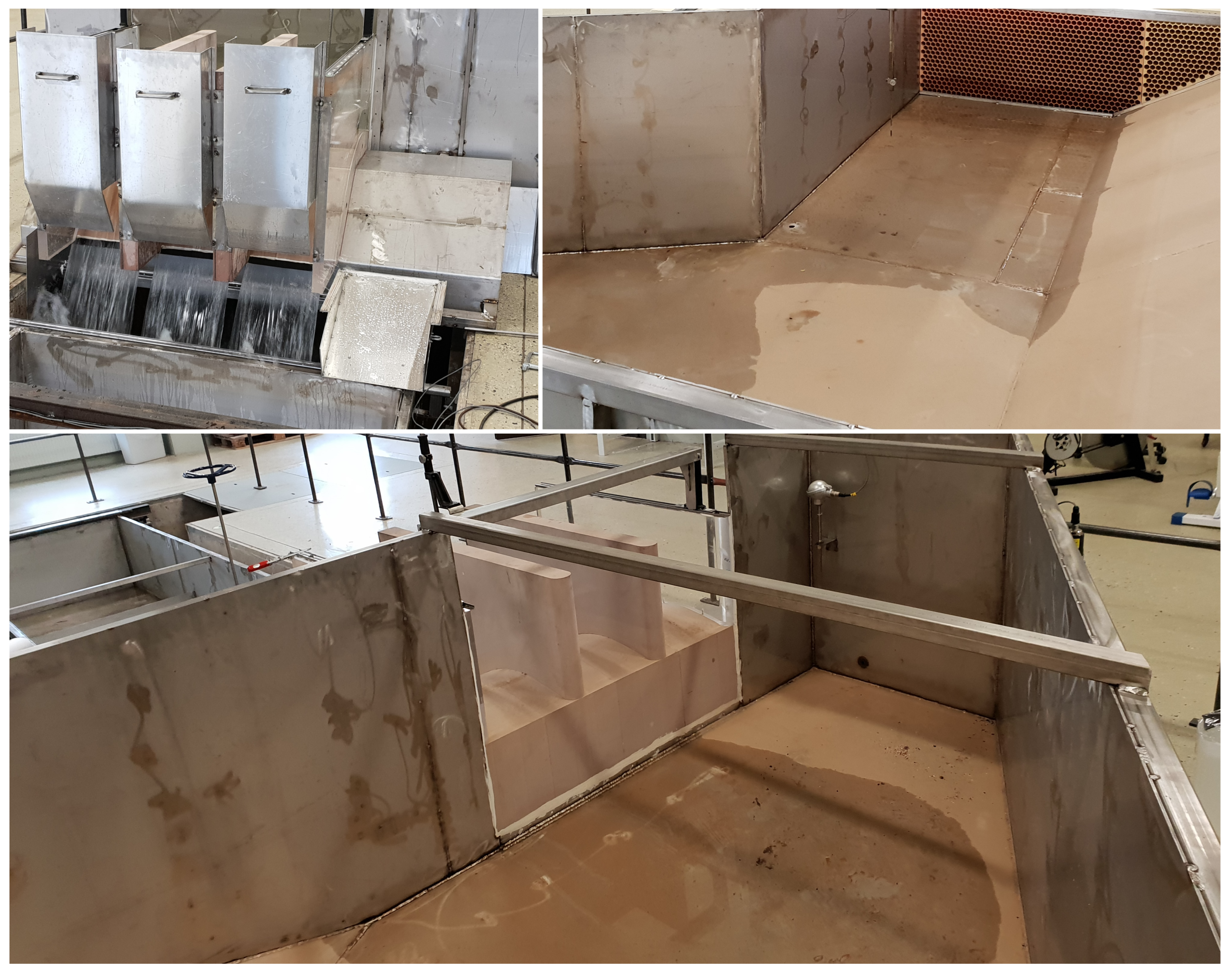
2.1. Experimental Setup

The experiments were performed at Vattenfalls hydraulic laboratory in Älvkarleby, Sweden. The channel consists of four parts with various instruments attached, the pump system, the channel, the spillways, and lastly the weight measuring tank. The pump system has two pumps that can be connected to it with, supplying a possible volume flow rate of 300 L per second, it leads into the channel from above, see Figure 1.

In the pipes leading from the pumps, there are devices for measuring of the flow, one for each pump. This experiment differs in the inlet conditions as new pipes were drawn from the pumps to the channel which can be seen in Figure 1, as well as increased flow. Several plates of perforated steel are situated close to the exit of the pipe so as to even out the incoming flow; the setup can be seen in Figure 1. A honeycomb structure is the final flow-regulating structure, and it is there to provide turbulence with a fixed length scale. This information can be used as a boundary condition for CFD analysis. Measuring the water level with no flow from the pumps shows a slight deviation to below zero in the data from the pumps, but well within the range of earlier calibration studies which showed a possible measurement error of ±1%. Inspecting a data series recording the closing of the valves to the channel shows a short delay of about 2–3 s depending on where in the pool the measurements are taken. Changes that are recorded by the instruments occur in the water level depending on the distance to the inlet. The channel has a sloped wall on one side and leading up to the spillway it moves past a corner with a sharp angle and widens past the outlets, this corner and the honeycomb can be viewed in Figure 2. The dimensions for the channel were 2 m wide at the honeycomb this width was kept for 3 m until a corner, after the corner it widens out to 5 m. The distance from the corner to the wall with the spillway was, according to the blueprint 2.36 m. The depth of the channel measured from the threshold of the spillway was 0.4 m and the distance from the threshold to the crest of the spillway was 0.035 m, some of the distances can be found in Figure 3. The three spillways have their geometry sourced from the hydropower plant at Torpshammar Sweden. Only the shape of the ogee spillway outlets was copied and the scale used was 1:50. Manufacturing defects resulted in slight differences between the different outlets of up to 3 mm, which is within 1% of the intended width of 30 cm. Within the channel, water is diverted through holes to three magnetostrictive sensors to monitor the water level in the channel see Figure 3 for the positions of the sensors. The measuring of the flow through the specific spillway outlets is accomplished by redirecting the flow by use of a sloped box structure that can be positioned underneath the different spillway outlets. This box leads the water into a 6 m³ tank suspended on four weight cells. Internal testing of the weight cells showed an uncertainty of ±0.1%, drift of the sensor which was compensated for in the post-processing of the results. The input from the weight cells is recorded with the software Labview from National Instruments together with data from the magnetostrictive sensors, temperature gauge, and volume flow rate provided by the pumps. The water in the system is stored in a reservoir underneath the floor. The water is redirected into the measuring tank for 60 ± 20 s. As the recording captures data before and after water is diverted into the measuring tank, an interval of at least 30 s in the middle of it is taken for data analysis, when possible more time is used. The average duration of the measurement used is 51.5 s. Due to the limited size of the tank used to gather water, the possible time for the larger flow rates limits recording time. A comparison of shorter time series to the longer ones shows differences within the error range of the instruments. The weight of the water in the tank is plotted against time, and the angle of the slope then provides an accurate measurement of the flow through the individual spillway outlets. This is repeated for all three spillway outlets with constant flow delivered from the pumps. The measured flow can be compared to the incoming flow measured from the pumps, giving a percentage of the total flow that passes through each individual outlet. Calibration is conducted by blocking all but one of the outlets and adjusting the signal from the weight tank to match the inlet volume flow. Data were gathered for each individual outlet and then repeated for that specific inflow three times, this was repeated over three days. This provided a total of nine sets of data for each low inflow case and a set of five for the 200 L per second case. When data were gathered there was water not flowing where intended due to leaks in the interface between the outlet and the weighing tank. Efforts were made to rectify this and to ensure that the correct values were documented. To this end, data were recorded for a low flow with and without sealing of the contraption used to redirect flow, the results are documented in

Table 1. Tests of the sealing of the redirection box. First two tests are made with an unsealed box, latter two with seals.

Inflow	Out1	Ratio1 %	Out2	Ratio2 %	Out3	Ratio3 %	W, H (mm)	SumRatio %
61.86	20.48	33.11	20.20	32.68	20.55	33.19	148.07	98.98
61.81	20.20	32.67	20.25	32.82	20.72	33.48	147.99	98.97
61.79	20.71	33.57	20.37	32.97	20.70	33.45	148.04	99.99
61.92	20.82	33.55	20.49	33.10	20.57	33.29	148.15	99.94

.

As can be seen in Table 1, specifically at the flow through outlet 3 leakage had less impact on the final results. Outlet 2 also shows a smaller impact of the sealing when compared to outlet 1. A possible cause for this is the small angle of the rails that the redirection box lies on. This results in a smaller impact of poor sealing on the accuracy of measurements of outlet 3 while outlets 1 and 2 may be more prone to errors if sealing is poorly performed, or ripped off during the experiment by friction while moving the contraption.

To capture the flow at relevant points in the channel Acoustic Doppler Velocimetry was chosen as a tool, as it has seen rigorous use in the literature, some examples include [20,21], where ADV has been used in smaller channels to record flow velocities around submerged obstacles. The tool has also seen use in measurements at larger scales, see [22]. The ADV used was a Nortek 10 MHz Velocimeter, data were recorded over one minute with a recording frequency of 100 Hz. In the literature, the time used for recording with ADV varies, [20], used 5 min, [21] used 3 min, while [23] used 4 min. To evaluate the quality of the data gathered, the inspection of histograms of the velocity distribution was conducted as in [24]. The probe consists of one transmitter and four receivers. Each pair of receivers measures data for two sets of velocity components. The U-component corresponds to the X direction, the V-component to the Y direction, and the W-component to the Z direction as shown in Figure 3. The ADV has four prongs, of which two are used for the U-component and two for the V-component; the W-component is measured for both pairs of prongs resulting in two measured sets that can be averaged to attain the actual W-component, this was not conducted and the W-component used is the one coupled with the U-component. Since the probe has to be inserted into the flow, ADV is a relatively intrusive method. However, the system requires no laser and usually no artificial seeding, sufficient particulate matter was suspended in the water and no artificial seeding was needed for quality data. The ADV data were taken at five locations 5 cm out from the outlets shown as red dots in Figure 3, 1 point in the middle of each outlet and 1 point at the midpoint between the outlets. For all points a vertical pillar of measurements was made, starting at a depth of 19 cm from the bottom and going up to 9 cm from the surface given by the pressure sensor closest to outlet 3.

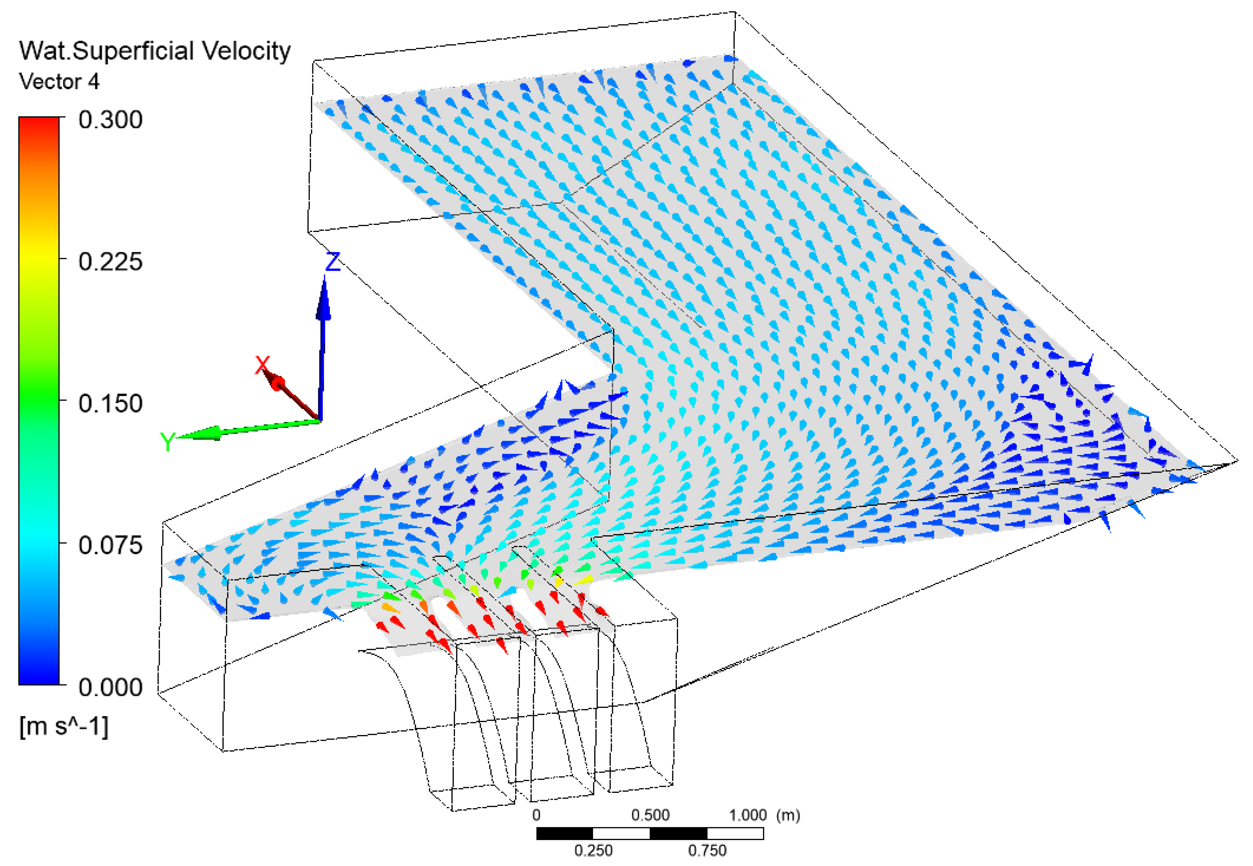
2.2. Numerical Setup

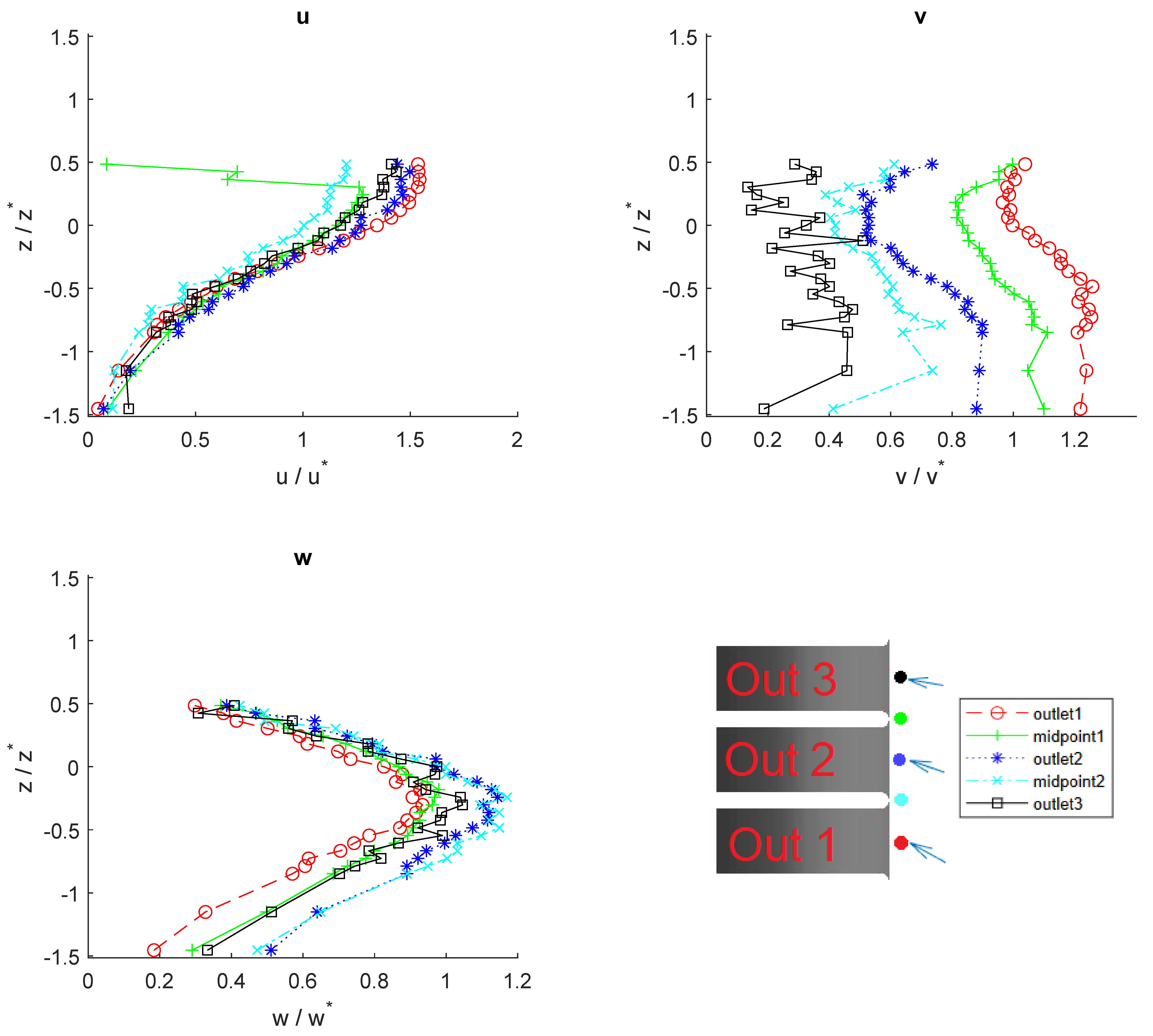
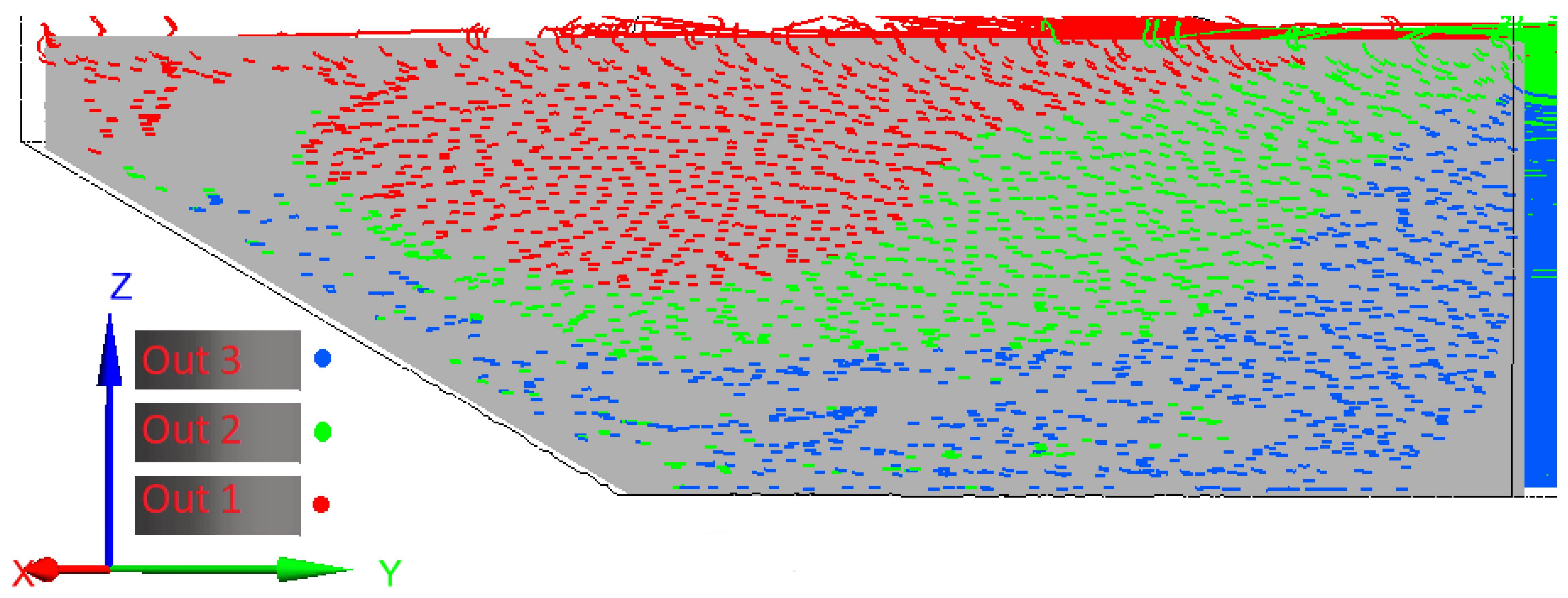
A model of the experiment was made from CAD blueprints, and verified by laser scanning of the geometry. Some small discrepancies were found in the range of ±1 cm for the main channel. To convert this geometry, ICEM CFD 19.0 was used, the same program also discretized the computational domain into a mesh. The mesh was made according to previously documented work on a similar setup, see [25], the documented work included a mesh independence study. The final mesh was created as a tetramesh with a hexacore, with a total of 5 million nodes. The k-epsilon turbulence model was used along with the volume of fluid method for the interaction of air and water. The walls are made of stainless steel and set as boundaries with smooth walls and a no-slip condition. The inlet conditions used were volume inflow, using a step function with water height taken from the experiments, to partition the inlet into water and air. The timestep used was 0.005 s, and the convergence criteria for the outer coefficient loop were RMS 5 × 10⁻⁵ for each timestep. The solver used was ANSYS CFX 2020 R2. A view of the setup is shown in Figure 4 showing the layout with arrows on the surface representing the surface velocity field.

3. Results

The data of the flow distribution in the spillway were gathered for the flow cases, and are shown in

Table 2. Inflow and outflow are in L/s. Ratio as percentage of recorded outflow to mean inflow for each specific outlet. Lastly shown is the summed ratios to establish amount lost to errors.

Inflow	Out1	Ratio1 %	Out2	Ratio2 %	Out3	Ratio3 %	ΣRatio %
90.50	30.31	33.52	30.01	33.11	30.36	33.56	100.19
90.55	30.47	33.67	30.24	33.40	30.64	33.82	100.89
90.43	30.31	33.49	29.94	33.14	29.88	33.03	99.66
90.49	30.32	33.53	30.06	33.22	30.22	33.37	100.12
90.33	30.38	33.68	30.08	33.30	30.26	33.46	100.44
90.30	30.34	33.64	30.13	33.34	30.30	33.53	100.51
90.35	30.28	33.49	29.94	33.15	30.07	33.30	99.94
90.41	30.14	33.34	30.05	33.25	30.08	33.25	99.84
90.34	29.95	33.15	30.08	33.30	30.10	33.31	99.76
99.27	33.14	33.41	32.97	33.17	33.06	33.32	99.90
98.80	32.73	33.32	32.68	33.08	33.03	33.25	99.65
99.12	33.32	33.60	33.05	33.34	33.37	33.68	100.62
100.02	33.67	33.62	33.28	33.31	33.21	33.21	100.14
100.17	33.41	33.45	33.33	33.23	33.51	33.39	100.07
100.77	33.78	33.68	33.62	33.20	33.83	33.56	100.44
99.55	33.52	33.65	33.24	33.31	33.09	33.34	100.30
99.53	32.84	32.98	32.94	33.16	32.99	33.10	99.24
99.68	33.44	33.55	33.08	33.17	33.00	33.12	99.84
109.64	36.72	33.41	36.86	33.66	36.32	33.16	100.23
109.78	36.80	33.51	36.39	33.12	36.50	33.29	99.92
109.59	36.57	33.39	36.41	33.23	36.53	33.30	99.92
109.49	36.97	33.71	36.09	33.06	36.49	33.27	100.04
109.46	36.76	33.61	36.50	33.27	36.35	33.25	100.13
109.26	36.59	33.43	36.37	33.28	36.41	33.40	100.11
109.83	36.84	33.57	36.39	33.11	36.54	33.27	99.95
109.78	36.51	33.24	36.33	33.12	36.36	33.10	99.46
109.80	36.57	33.30	36.22	33.00	36.52	33.23	99.53
200.46	66.05	32.99	67.31	33.53	67.59	33.71	100.23
200.33	64.70	32.25	66.54	33.25	67.15	33.53	99.03
199.93	65.71	32.90	67.19	33.53	66.97	33.53	99.96
199.46	65.89	33.04	67.05	33.58	66.94	33.59	100.21
199.39	67.03	33.53	66.71	33.54	65.65	32.92	99.99

. For comparison the gathered data were averaged, which can be seen in

Table 3. For easier overview of the difference between the high flow case and the lower flow cases. With addition of results from the simulations marked by (sim).

Mean Inflow	Mean Out1	Mean Ratio1	Mean Out2	Mean Ratio2	Mean Out3	Mean Ratio3	ΣRatios
90.41	30.27	33.50	30.05	33.24	30.21	33.40	100.14
99.65	33.31	33.47	33.13	33.21	33.23	33.33	100.01
109.62	36.70	33.46	36.39	33.20	36.44	33.25	99.91
110 (sim)	37.06	33.69	37.07	33.70	35.72	32.47	99.86
199.91	65.87	32.94	66.96	33.48	66.86	33.45	99.87
200 (sim)	66.45	33.22	67.66	33.83	65.89	32.94	99.99

.

The data sets in Table 2 show some variations, and two distinct outliers in the sum of ratios. One for the 90 L/s flow case and one for the 200 L/s flow case. The second 200 L/s case should have a simple explanation, the sealing was insufficient for the recording of outlet 1. The 90 L/s case shows the largest summed results for all outlets in the series at $100.89\%$. Due to the time-dependent nature variation in the flow has to be accepted as comparing the ratios to the other tests, for outlet 1, and outlet 2 there are other larger ratios recorded, while for outlet 3 it is the largest ratio. Regardless, none of the summed ratios show a deviation beyond what could be expected due to the error range of the instruments which would have to deviate by more than 1%. For comparison with the CFD results the data gathered and shown in Table 2 were averaged and presented next to data from the two simulations conducted in Table 3. It is quite clear that the simulations are not accurately predicting how the flow is distributed, at least not for the higher flow case as subtracting the CFD averages from the experimental data results in a difference between the outlets as follows: Outlet 1, −0.58 Outlet 2, −0.7 Outlet 3, 0.97 L/s. Expected errors due to instruments would be 1% of the flow through the outlets, with even flow through all outlets this would be 0.666...L/s for the 200 L/s case. Outlet 1 and 2 are on the edge of the error range while the difference in outlet 3 is clearly outside of the range of errors from the instrumentation. The water level in the channel was recorded at three different points, shown in Figure 3. Recorded data can be observed in

Table 4. Table of recorded average water levels for given average inlet flows. Height point 1 located before the bend, height point 2 right after the bend, height point 3 at the end of the channel. Also included are the differences between simulations, marked (sim) and experimental cases for the 110 and 200 L/s cases.

Average Flow (L/s)	Height Point 1 (mm)	Height Point 2 (mm)	Height Point 3 (mm)
90.42	181.78	181.74	182.34
99.66	191.91	191.72	192.43
109.63	202.59	202.35	203.21
110 (sim)	205.82	205.49	206.01
199.91	284.64	283.8	285.5
200 (sim)	286.86	286.01	287.6
Difference %
0.34	1.58	1.54	1.37
0.05	0.78	0.78	0.74

. Included in the table are the corresponding water levels from the two simulations for comparison. Of note is the slight overshoot for the simulations even accounting for the discrepancies in inflow as both experimental cases have slightly lower flow than their simulated counterparts. Unlike the discrepancies in how the flow is distributed, for the water level the difference between the experiments and the simulation is quite uniform, showing deviations while retaining the correct relative water level with the highest water level found in point 3 and lowest for point 2 for both the simulation and the experiments.

The ADV data are taken at five different points, 5 cm out from the outlets. One point in the middle of each outlet and 1 point at the midpoint between the outlets, these points are marked in Figure 3. Some differences can be seen in the ADV data from the outlets, as the velocities leading up to the outlets are different for each individual outlet. The ADV data taken indicate how the water flows into the different outlets and the mean values are plotted and shown in Figure 5. As for the first outlet, most of the water is drawn in close to the surface, while closer to the bottom it is moving towards the outlets further down. The points in between the outlets show lower velocities of the flow towards the outlets, with the point in between outlet 2 and outlet 3 showing larger fluctuations. The data as a whole show water close to the bottom moving to outlet 3 as the velocities in the z direction steadily increase towards that outlet while velocities in the x direction taper off. For the outlet measurements recorded, an SnR of 5 and a correlation of 70 were deemed acceptable as per recommendations from the manual [26], as the average velocities were the important variable.

For comparison between experimental data and simulations, the ADV data are normalized. The z-direction is normalized by the average hydraulic head above the crest given by the pressure sensors. The measured water column does not reach the hydraulic head as the water level is lower close to the spillway. For the simulations, monitor points were placed to mimic the positions of the experimental sensors to provide a hydraulic head to normalize. The respective velocities are normalized by the maximum velocity at the crest. For the velocities in the X-direction the largest velocity is found at outlet 1 so the rest of the velocities in the X-direction are normalized by that velocity, this method is used for the three respective velocities. The normalized ADV data and a corresponding simulation can be seen in Figure 6. The simulation data do not match the ADV data, the largest discrepancy can be noticed in the u velocities outside outlet 3. A trend for v and w velocities is that they show better agreement above the crest.

4. Discussion

The accuracy of the results was good with possible errors occurring due to faults during calibration, measurements of the water level were possibly accosted by such. For the lower flow case, the summation of the flow ratios is all close to 100%, as can be seen in Table 2. An explanation for the larger than 100% results could be that the recordings were conducted one outlet at a time, and the difference between the recordings shows that the flow is not constant through the outlets. As the potential error from the equipment is at 1%, they can be seen as accurate as a whole considering the variation in flow over time. For the specific distribution between the outlets, there were small differences recorded, and they persisted for most of the recorded low-flow cases. The flow through outlet 1 is higher than for the other outlets by a small margin of less than 1%. This is followed by a middling flow through outlet 3, and the least amount passing through outlet 2. The change as the flow is increased, seen in the 200 L/s case, contrasts with the CFD cases where the distribution remains the same for low and high cases. As the velocities increase for the higher flow case a possible reason for the relative reduced flow through outlet 1 in the experiment is the impact of flow separation around the leading corner of outlet 1, as with increased flow the lateral velocities increase. In the ADV data comparison to the simulation, it was shown that correct velocities could not be reproduced by the simulation below the threshold. This could be an indication that the flow at distances further away than the 5 cm measured by the ADV is not representative of what happens in the experiment. Larger flows result in higher velocities and more intense turbulence which is handled worse by the turbulence model. As the flow distribution between the outlets is not captured correctly, the potential faults in the setup must be discussed. The most glaring issue would be the inlet conditions at the honeycomb. By visual inspection during the experiment, the profile seems inverted to what could be expected of channel flow, showing higher velocities close to the channel walls as compared to the center of the channel. By backtracking streamlines from the outlets in the simulations, see Figure 7 it can be seen that outflow through the middle outlet is drawn from the center of the channel. This is likely a large contributing factor to the discrepancies between the simulations and the experiments. Other possible contributions could be the computational mesh and the turbulence modeling, as the corner in the middle of the channel sheds visible vortexes which the k-epsilon model has trouble resolving. Additionally, there are two recirculation zones, these zones can be seen in Figure 4, one being along the opposite wall of the spillway, with a smaller one being in the corner to the left of the spillway from the perspective of Figure 4. As this experiment is made on a smaller scale, the impact of scale effects should be considered, according to [27] a minimum of 0.03 m was needed for an upstream head to avoid head-discharge size scale effects due to surface tension and viscous effects for a similarly sized experiment for flow over wiers. Air entrainment in the outlets was deemed negligible as no noticeable entrainment occurred before the water reached the equipment used to redirect the water. Comparing the results of the flow behavior in front of the outlets with the distribution of flow through the outlets shows that the accurate modeling of the flow behavior is not as simple as capturing the correct surface level. Further research should include recordings of the inlet, and possible cross sections of velocity closer to the outlets. A relevant question is if it is possible to gather data from open spillways close enough to replicate such experiments. If it is untenable is it worth the effort to explore that avenue? Is it worth gathering data that close to an open spillway? Are they even usable, or good enough to justify the added expense? Using static pressure as an inlet condition is unlikely to predict the correct inlet and outlet flows. Earlier documentation [28] mentions that the significance of the contribution for the velocity head depends on the relation of height over the crest to height over the floor of the approach channel, the key metric mentioned being less or equal to one. For this experiment, the highest value of the ratio is for the 200 L/s case with a ratio of 249 mm/435 mm = 0.57, (heights were taken from the simulation). The lowest ratio being $0.34$, the change from 90 L per second to 200 L per second is quite large and can be a reason for the larger differences.

5. Conclusions

We show that it is possible to accurately capture flow distribution for an experimental model with complicated inlet conditions and several outlets for a wide range of flows. The water levels in the simulations show good agreement with the recorded values in the experiments for the higher flow case of 200 L/s, while the lower case of 110 L/s differs more; some discrepancies are most likely due to the difference in inlet flow. Any errors lie within the uncertainty of the instrumentation when accounting for the previously mentioned inlet flow discrepancy. Simulating correct flow distribution seems a more difficult endeavor. This leads to the conclusion that the prediction of water levels is a simpler task, and less dependent on correct inlet and boundary conditions. This should reassure hydropower dam owners of the validity of CFD as a tool for evaluating discharge capacity for a given reservoir inflow. There are multiple possible reasons for the lack of accuracy in predicting how the flow is distributed, such as velocities over the inlet, and an unsuitable turbulence model. Further research is needed to clarify the requirements for accurate simulations with regard to the distribution of flow. Future experiments with changes to the geometry to induce a larger difference in flow between the outlets should be conducted to provide cases for validation and verification. Accompanying these, further simulations will be conducted with more boundary conditions based on ADV measurements and more advanced turbulence models.

References

1. Hellgren, R.; Bartsch, M. Book on Dams the Swedish Experience. Available online: https://www.svk.se/siteassets/3.sakerhet-och-beredskap/dammsakerhet/vagledningar-och-stod/book_on_dams.pdf (accessed on 15 March 2024).
2. Yang, J.; Patrik, P.; Teng, P.; Xie, Q. The Past and Present of Discharge Capacity Modeling for Spillways—A Swedish Perspective. Fluids 2019, 4, 10. [Google Scholar] [CrossRef]
3. Peltier, Y.; Dewals, B.; Archambeau, P.; Pirotton, M.; Erpicum, S. Pressure and velocity on an ogee spillway crest operating at high head ratio: Experimental measurements and validation. J. Hydro-Environ. Res. 2018, 19, 128–136. [Google Scholar] [CrossRef]
4. Solheim, N.; Hedberg, P.A.M.; Lunde, H.; Pummer, E.; Lia, L. Modified Guide Walls for Incremental Increase of Spillway Capacity. In Proceedings of the 40th IAHR World Congress, Vienna, Austria, 21–25 August 2023; pp. 1978–1983. [Google Scholar]
5. Stilmant, F.; Erpicum, S.; Peltier, Y.; Archambeau, P.; Dewals, B.; Pirotton, M. Flow at an Ogee Crest Axis for a Wide Range of Head Ratios: Theoretical Model. Water 2022, 14, 2337. [Google Scholar] [CrossRef]
6. Mozaffari, S.; Amini, E.; Mehdipour, H.; Neshat, M. Flow Discharge Prediction Study Using a CFD-Based Numerical Model and Gene Expression Programming. Water 2022, 14, 650. [Google Scholar] [CrossRef]
7. Kocaer, Ö.; Yarar, A. Experimental and Numerical Investigation of Flow Over Ogee Spillway. Water Resour. Manag. 2020, 13, 3949–3965. [Google Scholar] [CrossRef]
8. Savage, B.; Johnson, M. Flow over ogee spillway: Physical and numerical model case study. J. Hydraul. Eng. 2001, 8, 640–649. [Google Scholar] [CrossRef]
9. Johnson, M.; Savage, B. Physical and Numerical Comparison of Flow over Ogee Spillway in the Presence of Tailwater. J. Hydraul. Eng. 2006, 12, 640–649. [Google Scholar] [CrossRef]
10. Andersson, A.G.; Andreasson, P.; Lundström, T.S. CFD-Modelling and Validation of Free Surface Flow During Spilling of Reservoir in Down-Scale Model. Eng. Appl. Comput. Fluid Mech. 2013, 7, 159–167. [Google Scholar] [CrossRef]
11. Lee, J.H.; Julien, P.Y.; Thornton, C.I. Interference of Dual Spillways Operations. J. Hydraul. Eng. 2019, 10, 142–149. [Google Scholar] [CrossRef]
12. Li, L.; Xu, W.; Tan, Y.; Yang, Y.; Yang, J.; Tan, D. Fluid-induced vibration evolution mechanism of multiphase free sink vortex and the multi-source vibration sensing method. Mech. Syst. Signal Process. 2023, 189, 110058. [Google Scholar] [CrossRef]
13. Li, L.; Li, Q.; Ni, Y.; Wang, C.; Tan, Y.; Tan, D. Critical penetrating vibration evolution behaviors of the gas-liquid coupled vortex flow. Energy 2024, 292, 130236. [Google Scholar] [CrossRef]
14. Li, S.; Yang, J.; He, X. Modeling transient flow dynamics around a bluff body using deep learning techniques. Ocean Eng. 2024, 295, 116880. [Google Scholar] [CrossRef]
15. Kadia, S.; Lia, L.; Albayrak, I.; Pummer, E. The effect of cross-sectional geometry on the high-speed narrow open channel flows: An updated Reynolds stress model study. Comput. Fluids 2024, 271, 106184. [Google Scholar] [CrossRef]
16. Li, S.; Cain, S.; Wosnik, M.; Miller, C.; Kocahan, H.; Wyckoff, R. Numerical Modeling of Probable Maximum Flood Flowing through a System of Spillways. J. Hydraul. Eng. 2011, 137, 66–74. [Google Scholar] [CrossRef]
17. Zeng, J.; Zhang, L.; Ansar, M.; Damisse, E.; González-Castro, J.A. Applications of Computational Fluid Dynamics to Flow Ratings at Prototype Spillways and Weirs. I: Data Generation and Validation. J. Irrig. Drain. Eng. 2017, 143, 04016072. [Google Scholar] [CrossRef]
18. Yildiz, A.; Yarar, A.; Kumcu, S.Y.; Marti, A.I. Numerical and ANFIS modeling of flow over an ogee-crested spillway. Appl. Water Sci. 2020, 10, 90. [Google Scholar] [CrossRef]
19. De Morais, V.H.P.; Gireli, T.Z.; Vatavuk, P. Numerical and experimental models applied to an ogee crest spillway and roller bucket stilling basin. Braz. J. Water Resour. 2020, 25, e18. [Google Scholar] [CrossRef]
20. Jeon, J.; Kim, Y.; Kim, D.; Kang, S. Flume Experiments for Flow around Debris Accumulation at a Bridge. KSCE J. Civ. Eng. 2024, 28, 1049–1061. [Google Scholar] [CrossRef]
21. Pandey, M.; Sharma, P.K.; Ahmad, Z.; Singh, U.K.; Karna, N. Three-dimensional velocity measurements around bridge piers in gravel bed. Mar. Georesources Geotechnol. 2018, 36, 663–676. [Google Scholar] [CrossRef]
22. Mikael, H.; Gunnar, H.; Nils, S. Experimental and Computational Evaluation of Fish Passageway with Porous Media Boundary. In Proceedings of the 40th IAHR World Congress, Vienna, Austria, 21–25 August 2023; pp. 2422–2428. [Google Scholar]
23. Singh, U.K.; Ahmad, Z.; Kumar, A. Turbulence characteristics of flow over the degraded cohesive bed of clay–silt–sand mixture. ISH J. Hydraul. Eng. 2017, 3, 308–318. [Google Scholar] [CrossRef]
24. Ömer, K. Distribution of turbulence statistics in open-channel flow. Int. J. Phys. Sci. 2011, 6, 3426–3436. [Google Scholar]
25. Hedberg, M.; Hellström, G.; Andreasson, P.; Andersson, A.G.; Angele, K.; Andersson, R. Numerical modelling of flow in parallel spillways. In Proceedings of the 8th IAHR International Symposium on Hydraulic Structures ISHS2020, Santiago, Chile, 12–15 May 2020; Volume 1. [Google Scholar]
26. Nortek, A.S. The Comprehensive Manual for Velocimeters; Nortek AS: Rud, Norway, 2018; Available online: https://www.nortekgroup.com/assets/software/N3015-030-Comprehensive-Manual-Velocimeters_1118.pdf (accessed on 15 March 2024).
27. Erpicum, S.; Tullis, B.P.; Lodomez, M.; Archambeau, P.; Dewals, B.J.; Pirotton, M. Scale effects in physical piano key weirs models. J. Hydraul. Res. 2016, 6, 692–698. [Google Scholar] [CrossRef]
28. USACE. Hydraulic Design of Spillways; U.S. Army Corps of Engineers: Washington, DC, USA, 1990. [Google Scholar]
Figure 1. Pipe system leading water into the channel.
Water 16 00871 g001
Figure 2. Top left, outlets, redirection box, and opening of weighing tank. Top right, honeycomb with empty channel. Bottom, channel leading up to the outlets.
Water 16 00871 g002
Figure 3. Schematic of experimental setup with ADV positions marked with red dots at the spillway. Positive x direction is against the flow direction, marked by a red arrow. Negative direction towards sloping side wall. Honeycomb position shown by the orange rectangle. Water holes for the magnetostrictive sensors shown with red squares. Weight cells marked with blue squares. Included is a side view of the spillway part of the geometry showing the depth of the channel.
Water 16 00871 g003
Figure 4. Isometric view of the simulation from CFX-post, showing surface velocities along an isosurface representing VOF = 0.5 shown in grey for 110 l/s simulation.
Water 16 00871 g004
Figure 5. ADV data at outlets and midpoints. Included is an illustration of where the ADV was used color-coded. Scaling explained below.
Water 16 00871 g005
Figure 6. Simulation results compared to ADV data. Horizontal errorbars show one standard deviation of the ADV data. Arrows based on the ADV data indicating direction of the water heading towards the outlets.
Water 16 00871 g006
Figure 7. Streamlines from inlet to the three different outlets from simulation with 110 L/s as inlet flow, red for outlet 1, green for outlet 2, blue for outlet 3.
Water 16 00871 g007