Article

Joint Failure Probability of Dams Based on Probabilistic Flood Hazard Analysis

by
Matthew G. Montgomery
1,*,
Miles B. Yaw
1 and
John S. Schwartz
2
1
Tennessee Valley Authority, Knoxville, TN 37902, USA
2
Department of Civil and Environmental Engineering, Tickle College of Engineering, University of Tennessee Knoxville, Knoxville, TN 37916, USA
*
Author to whom correspondence should be addressed.
Water 2024, 16(6), 865; https://doi.org/10.3390/w16060865
Submission received: 9 February 2024 / Revised: 13 March 2024 / Accepted: 15 March 2024 / Published: 17 March 2024

Abstract

:
Probabilistic risk methods are becoming increasingly accepted as a means of carrying out risk-informed decision making regarding the design and operation policy of structures such as dams. Probabilistic risk calculations require the quantification of epistemic and aleatory uncertainties not investigated through deterministic methodologies. In this hydrological study, a stochastic sampling methodology is employed to investigate the joint failure probability of three dams in adjacent similarly sized watersheds within the same hydrologic unit code (HUC) 6 basin. A probabilistic flood hazard analysis (PFHA) framework is used to simulate the hydrologic loading of a range of extreme precipitation events across the combined watershed area of the three studied dams. Precipitation events are characterized by three distinct storm types influential in the Tennessee Valley region with implications for weather variability and climate change. The stochastic framework allows for the simulation of hundreds of thousands of spillway outflows that are used to produce empirical bivariate exceedance probabilities for spillway discharge pairs at selected dams. System response curves that indicate the probability of failure given spillway discharge are referenced for each dam and applied to generate empirical bivariate failure probability (joint failure probability) estimates. The stochastic simulation results indicate the range of spillway discharges for each pair of dams that pose the greatest risk of joint failure. The estimate of joint failure considering the dependence of spillway discharges between dams is shown to be three to four orders of magnitude more likely (7.42 × 10² to 5.68 × 10³) than estimates that assume coincident failures are the result of independent hydrologic events.

1. Introduction

The design of a structure within the flood plain may be dangerous or overly conservative if the uncertainty associated with risk factors is not quantified. Risk-informed decision making requires the quantification of uncertainties associated with calculation assumptions and the inherent variability of natural processes not investigated through deterministic methodologies [1]. Conventional methods for determining hydrologic criteria are often limited to observations at a single location in the case of risk studies at dams [2,3,4]. This research demonstrates an approach to extend conventional methodology for risk studies by evaluating the risk posed by a system of multiple dams in adjacent similarly sized watersheds through a single risk study; moreover, by using stochastic sampling to evaluate factors that contribute to hydrologic risk, the influence of dominant storm types on the hydrologic response is considered. Understanding the response of a system of dams to extreme storm events could improve risk estimates, inform reservoir storage regulation policies, and provide increased resiliency in response to weather variability and climate change.
The extension of conventional probabilistic flood hazard methodology to incorporate joint failure probabilities at multiple dams is a novel contribution to the stochastic flood modeling literature, although many studies have been conducted on multivariate flood frequency analysis and the use of a bivariate return period for hydrologic dam design applications [5,6]. Research on the hydrologic response of a system of dams indicates that overtopping and failure are significantly influenced by factors other than inflows due to interconnected system components such as initial reservoir levels, storage availability, and reservoir operations and discharge capabilities [7]. This research aims to build upon previously completed stochastic hydrological studies and demonstrate the interconnected nature of risk factors for a system of dams in parallel, namely the impact of coincident discharges that can occur at multiple dams during large storm events that impact adjacent watersheds.

1.1. Background

Routine risk assessments are implemented to determine, in part, whether dams are hydrologically adequate and how likely they are to fail under given conditions [1]. These assessments support risk-informed decision-making efforts related to the design, modification, and operation of dams by considering the frequency of hazardous events such as floods and earthquakes, the response of a dam to a hazard (failure mode), and the potential consequences of failure [8]. Hydrological adequacy is often defined based on reasonably conservative deterministic analysis methods, such as probable maximum flood (PMF), but such deterministic methods do not provide decision makers with critical information related to the likelihood of extreme events. Hydrologic loading probabilities are necessary to estimate failure likelihoods associated with potential failure modes that may be related to structural, geotechnical, or other related components of a dam. Hydrologic loading probabilities are therefore a critical component in the risk assessment of dams because they provide data used to evaluate the likelihood of hydrologically dependent potential failure modes. Hydrologic loading criteria that are often considered when assessing the risk of potential failure modes include the duration and frequency of inflows to a reservoir, the duration and frequency of pool elevations upstream of a dam, and the duration and frequency of outflows from a dam [1,8]. It is important to obtain an accurate estimate of the probability of these hydrologic loading variables, especially for loading conditions that could pose significant risk.
Early approaches for estimating hydrologic loading were limited to deterministic methods and the extrapolation of observed data. In an effort to promote uniform and consistent methods for determining flood flow frequency, the U.S. Water Resources Council, the Interagency Committee on Water Data, and U.S. Geological Survey published several bulletins, starting in 1967 and culminating most recently with Bulletin 17C “Guidelines for Determining Flood Flow Frequency” published in 2018 [3]. Early flood frequency estimation methods were proposed using the method of moments to fit the log-Pearson type III distribution to annual peak flow data. Later updates considered regional skew, outliers, and historical floods [9,10]. Following Bulletin 17B from the Interagency Committee on Water Data [10], the use of a conditional probability adjustment was introduced in separate studies [11,12]. Bulletin 17C provided updates to the generalized representation of flood data, an extension of the method of moments to accommodate interval data, and an approach for identifying low outliers in flood data [3,13].

1.2. Probabilistic Flood Hazard Analysis (PFHA)

Hydrologic hazard curves plot a hydrologic loading variable (peak discharge from a dam, total flood volume, peak reservoir stage, etc.) versus the annual exceedance probability (AEP) (the likelihood of that hydrologic loading variable value being met or exceeded in a given year). The process of developing hydrologic hazard curves for various hydrologic loading variables is referred to as probabilistic flood hazard analysis (PFHA). There are numerous approaches for developing hydrologic hazard curves. For example, the AEP may be calculated by statistical analysis of stream gage data [14], estimates from rainfall–runoff hydrologic models can be assessed with the assumption that the return period of a flood is equal to the return period of a precipitation event [15,16], stochastic rainfall–runoff modeling may be implemented to explicitly model hydrological responses [17,18], and paleo-flood records may be analyzed [19]. It is important to note that many of the methods mentioned here rely on the assumption that a rainfall event has an AEP value similar to an associated flood event; however, this assumption is often not verifiable [20,21].
Working from the concepts and procedures outlined in Bulletin 17C, entities such as the U.S. Army Corps of Engineers (USACE) have developed methodologies for determining hydrologic loading probabilities and assessing hydrologic hazards at dams, considering the variability associated with reservoir operations. The hydrologic hazard methodology outlined by USACE categorizes uncertainty as “natural variability” and “knowledge uncertainty” [1]. Natural variability associated with hydrological processes is modeled by sampling from a range of input parameters using a stochastic methodology as discussed in Section 1.3.1, while knowledge uncertainty is quantified through sampling uncertainty and model uncertainty. Hydrologic hazard studies carried out by USACE and others often aim at limiting uncertainty by obtaining as large a sample as possible for a hydrologic variable and ensuring that mathematical models fit available data sufficiently well. The sampling uncertainty decreases as the hydrologic variable period of record (sample size) increases, and the model uncertainty decreases if analytical probability distributions fit data well. The reduction of uncertainty serves to reduce the size of confidence intervals and produce more accurate hydrologic hazard curves [4].

1.3. Stochastic Modeling

1.3.1. Stochastic Modeling Overview

The lack of sufficient historical data, changes in reservoir storage regulation policies, climatic variability, and the need to assess extreme events has led to the widespread implementation of stochastic modeling. As mentioned in Section 1.2 above, the assumption that a precipitation event will have an AEP similar to an associated flood event (known as AEP neutrality) is often not verifiable or justifiable, but stochastic rainfall–runoff modeling offers a way to address this issue [4,20,21]. Stochastic modeling allows for inputs into a deterministic flood model to be treated as uncertain variables rather than fixed values. Estimates of flood frequency may be determined by randomly selecting model parameters, initial conditions, and precipitation inputs from defined precipitation frequency distributions [16,20]. Monte Carlo sampling techniques simulate the natural variation in hydrometeorological inputs and generate probability distributions associated with sets of model inputs. Consequently, a probability can be associated with a calculated hydrologic variable, since the impact of initial conditions, model parameters, and precipitation inputs that drive hydrologic risk are accounted for through the stochastic sampling. Key advantages of this stochastic sampling methodology include the ability to account for epistemic and aleatory uncertainties and estimate the likelihood of extreme loading conditions without relying on extrapolation from observed data or the assumption of AEP neutrality.

1.3.2. Stochastic Modeling Applications

The USACE has developed a methodology for implementing stochastic modeling for PFHA studies at dams using Risk Management Center Reservoir Frequency Analysis software (RMC-RFA). A stochastic approach is followed by allowing for variability through the sampling of inflow volume, inflow hydrograph shape, flood season, and reservoir starting stage. A two-looped nested Monte Carlo simulation is employed that simulates natural variability in the inner loop as a realization comprising thousands of flood events [1]. The result is a suite of hydrologic hazard curves useful for estimating probability across a range of hydrologic loading variables (peak discharge, total flood volume, peak reservoir stage, etc.). Many other examples of stochastic methodologies have been developed for risk studies at dams as well as other applications [4]. Stochastic simulations are used to extend reservoir pool stage frequency curves to peak elevations not previously recorded by evaluating the impact of initial reservoir conditions paired with extreme storm events. Lower stage values may be observed at a given AEP when compared with deterministic estimates with high levels of conservatism [2]. Similarly, stochastic storm generation techniques are used to estimate flood maps via Monte Carlo-based simulations, with results indicating that non-stochastic design storm events may overestimate flood maps in comparison with stochastic techniques that better characterize the spatial variability of rainfall [22]. Stochastic models incorporating historical river flows from global rainfall–runoff models may be used to compare relative flow exceedance probabilities rather than volumetric flow values from gage observations, better capturing the spatial patterns of flood events [23]. An increase in stochastic modeling has resulted in better understanding of the sensitivities in flood frequency analyses associated with components of the modeling framework. Precipitation inputs have been shown to contribute the most to variance in the case of rare floods, while initial conditions are the most influential as events become more frequent; moreover, the structure of the hydrologic model, as well as interactions between the hydrologic model structure and model parameters, play a significant role for specific basin characteristics and flood metrics [4].

1.3.3. The Stochastic Event Flood Model (SEFM)

Tennessee Valley Authority (TVA) has developed a PFHA system for use in risk studies at dams that employs the basic stochastic modeling approach outlined in the stochastic event flood model (SEFM) developed by MGS Engineering [18,24]. A detailed description of SEFM can be found in Section 2.2, and an overview is provided here. The approach detailed by the SEFM is extended and optimized to address the complexity of the TVA reservoir system made up of 49 dams in the Tennessee River watershed. This approach uses regional point precipitation frequency analyses for a given storm type over the study area containing the watershed of interest. Stochastic storm generation and storm transposition methods are used to develop precipitation frequency relationships with uncertainty bounds for a given storm type. Watershed conditions that influence the response to extreme events are sampled from a long-term simulation of synthetic hydrology and reservoir operations. A date from the long-term simulation is selected, and the watershed conditions associated with the date are used to define the starting conditions of the synthetic event. Monte Carlo sampling procedures are used to allow variation in hydrometeorological inputs like soil moisture content, reservoir starting elevation, sampled storm depth, and storm spatiotemporal characteristics. The stochastic framework uses a suite of hydrologic models representing the studied watershed in the stochastic flood routing and reservoir operations simulations [18,24]. An overview of the TVA PFHA system framework is shown in Figure 1.

1.3.4. Advantages of SEFM

There are three primary advantages regarding the use of SEFM for the TVA system when compared with other stochastic methods for developing hydrologic hazard curves. First, the SEFM approach offers a more computationally efficient solution, as it does not require the characterization of all aspects affecting a continuous time series of precipitation; rather, individual events expected to produce rare hydrologic responses can be selectively simulated through SEFM, as discussed in Section 2.3.1. This contrasts with the common approach of extracting annual maxima from a long-term simulation of a synthetically derived continuous precipitation time series run through watershed models such as by Steinschneider and Brown [25]. Second, the sampling of initial conditions from a long-term simulation in the SEFM framework eliminates the need for complicated statistical methods that may not sufficiently characterize the relationship between starting pool elevations and watershed moisture conditions in large watersheds with many reservoirs [26]. Finally, SEFM can be tailored to capture the influence of distinct storm types that are influential in the Tennessee Valley. Stochastic sampling of the spatial and temporal characteristics of different storm types produces a range of flood hydrograph shapes, runoff durations and volumes, and resulting peak discharges. Sampled storm types include mid-latitude cyclones (MLCs), tropical storm remnants (TSRs), and mesoscale storms with embedded convection (MECs), as discussed in Section 2.2.1.

1.4. Study Objectives

As the integration of risk-informed decision making has led to the increased implementation of PFHA for hydrologic hazard studies at dams, next steps are being taken to expand the applications of PFHA and adapt calculation frameworks to better characterize risk. The objectives of this study are to (a) use SEFM to assess the correlation of peak spillway discharges during individual storm events for three dams in adjacent similarly sized watersheds in the Tennessee Valley; (b) determine the bivariate exceedance probability for discharge pairs at associated dams, accounting for the influence of dominant storm types on the hydrologic response; and (c) determine the probability of coincident dam failures (joint failure probability) by taking into account the dependent response of dams to associated discharge pairs, thereby expanding the conventional PFHA analysis to characterize the risk posed by a system of dams versus an individual dam. By using PFHA to characterize system risk, a more comprehensive understanding of the factors that influence hydrologic response on a system level may be developed. Model parameters, initial conditions, and precipitation inputs can be assessed not only by the induced hydrologic response at a single location (e.g., [27]) but also by the correlation between responses at multiple locations. This correlated response may be critical when assessing the impact of extreme storm events on dams with adjacent drainage areas, especially in a resource constrained environment where the same small pool of labor is responsible for the care of multiple projects; moreover, understanding the response of a system of dams to extreme storm events could better inform reservoir storage regulation policies and provide increased resiliency in response to weather variability and climate change.

2. Data and Methods

2.1. Study Area

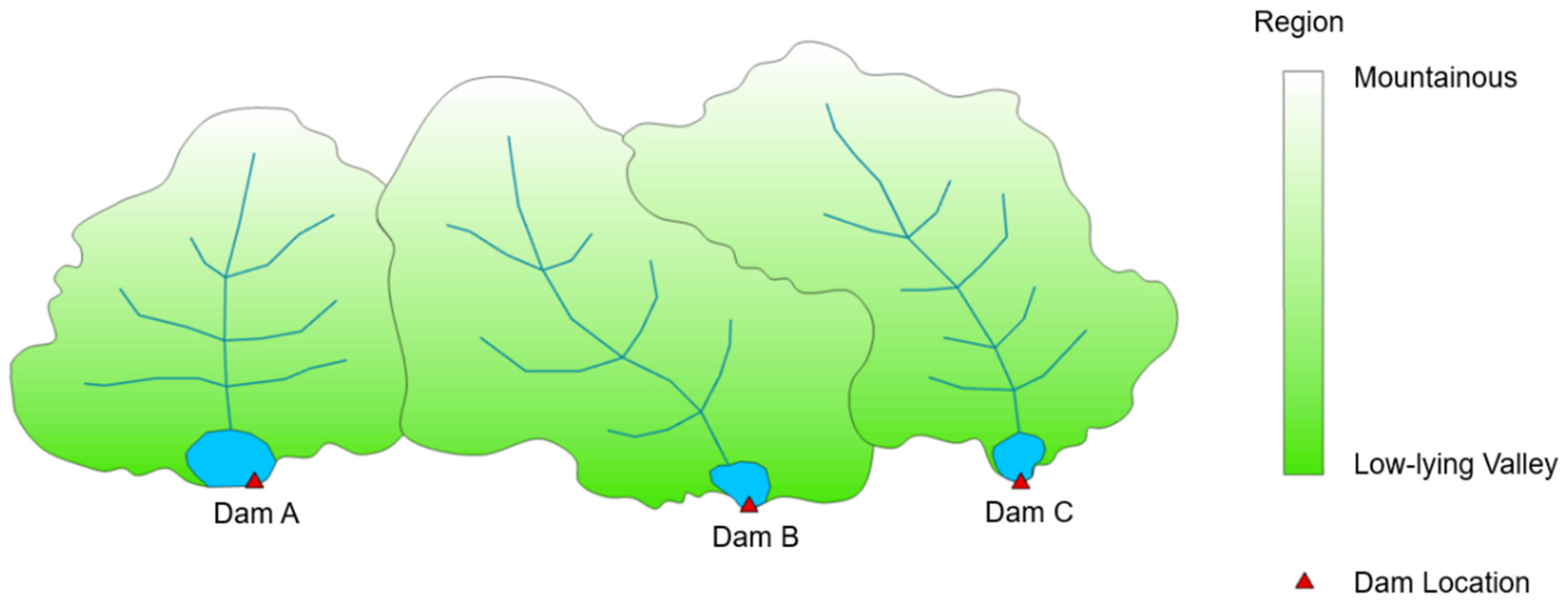
Hydrologic hazards were evaluated at three dams in adjacent similarly sized watersheds located within the Tennessee Valley region. The exact location of the dams will remain undisclosed; within this report the studied dams will be denoted as Dam A, Dam B, and Dam C. Each watershed has a total drainage area of less than 500 square miles, and all three watersheds are within the same hydrologic unit code (HUC) 6 basin. A generalized depiction of the study area portraying watershed characteristics and the relative location of each dam is shown in Figure 2.

2.2. Input Data for Stochastic Simulations

Essential to the development of hydrologic hazard curves is the method of stochastic sampling discussed in Section 1.3. This study used the TVA PFHA system to develop hydrologic hazard curves by employing the basic stochastic modeling approach of SEFM [18,24]. Initial conditions and model inputs were used to generate thousands of simulations, capturing the influence of extreme storm events across a range of storm templates and initial watershed conditions.
The following sections describe the inputs used for stochastic modeling. The five primary inputs included in the SEFM sampling routine described in Section 1.3.3 were as follows:
  • Watershed Precipitation Depth: The watershed precipitation depth was obtained from the precipitation frequency curve for a given storm (see Section 2.2.3). Precipitation sampling bins were specified across a defined sampling range for stratification of the precipitation frequency curve as described in Section 2.3.1.
  • Storm Templates: The spatial distribution of rainfall was obtained from defined storm templates for MLC, MEC, and TSR storms as described in Section 2.2.1 and Section 2.2.2. An AEP range was associated with each storm template, and relative weighting factors were applied to storm templates to determine sampling frequency.
  • Seasonality: the probability of specific storm types occurring at specific times of the year was defined based on historical observations within the Tennessee River watershed, influencing the likelihood of certain types of storms being sampled at specific dates in the long-term simulation.
  • Initial Conditions: soil moisture states, reservoir states, and river states were obtained from the long-term simulation.
  • Storm Insertion Dates: valid dates to insert storms were identified within the long-term simulation according to wet and dry periods and the storm type being sampled.

2.2.1. Storm Types

A representative sample of storms was needed to provide an unbiased estimate of the AEP for flood outputs, especially maximum releases from a spillway, which are directly influenced by maximum flood discharges related to spatial and temporal characteristics of storms at the scale of the studied watershed [28]. Different storm types are defined and investigated based on historically observed meteorological patterns to represent the spatial and temporal characteristics influencing the flood response for the watershed under investigation [29]. The following storm types were considered in this study:
  • Mid-Latitude Cyclones (MLCs): synoptic scale storms most commonly occurring in the winter period with extended durations and gradually varying precipitation gradients.
  • Tropical Storm Remnants (TSRs): decadent tropical storms that impact very large areas with low-to-moderate precipitation intensities generating large total precipitation volumes over several days, occurring during the Atlantic hurricane season.
  • Mesoscale Storms with Embedded Convection (MECs): commonly referred to as summer thunderstorms, smaller scale convective storms with high-intensity precipitation clusters of convective cells in addition to low-to-moderate intensity precipitation in areas surrounding convective cells, characterized by shorter durations and chaotic spatial distribution of precipitation.

2.2.2. Storm Templates

A suite of storm templates was assembled to represent the spatial and temporal characteristics influencing the flood response for the watershed under investigation. Temporal characteristics define the loading of a storm (front-loaded, middle-loaded, back-loaded) and hyetograph shapes. Spatial characteristics define the locations over which a storm will center and the distribution of heavier and lighter precipitation areas. As the size of a watershed increases, spatial characteristics become more important as the flood response times become longer and the number of major tributaries increases [30]. When developing storm templates for this study, the combined watershed area of the three dams was considered.
TVA’s storm database and transposition tool (SDTT) was used as a centralized database from which to access detailed precipitation analyses when developing storm templates for all storm types over the combined watershed area considered in this study. Storm templates referenced within the SDTT were developed according to the isopercental analysis methodology [31]. This methodology consists of transforming observed precipitation values in a mathematical space so that data can be linearly interpolated between observation sites, populating grid cells in a raster field constructed through geographic information system (GIS) mapping of the study area. The data can then be transformed back into real space to represent complex spatial patterns. The isopercental technique is particularly useful for analyzing large synoptic-scale storms in mountainous terrain where non-linear behavior is observed between precipitation data points, and can also be used for transposing storms from one location to another [31,32]. The five largest analyzed historical storms that occurred over the combined watershed were selected and supplemented by selecting other large historical storms that have occurred in the Tennessee Valley and transposing them to the combined watershed. The SDTT tool uses a cluster analysis to group and select storms over a representative range of characteristics, and weighting factors are assigned to define the frequency that each storm template is sampled in the stochastic modeling. Weighting factors are assumed based on the historical frequency of large storms in the region and are selected to maintain the expected frequency of specific storm patterns.

2.2.3. Precipitation Frequency Relationships

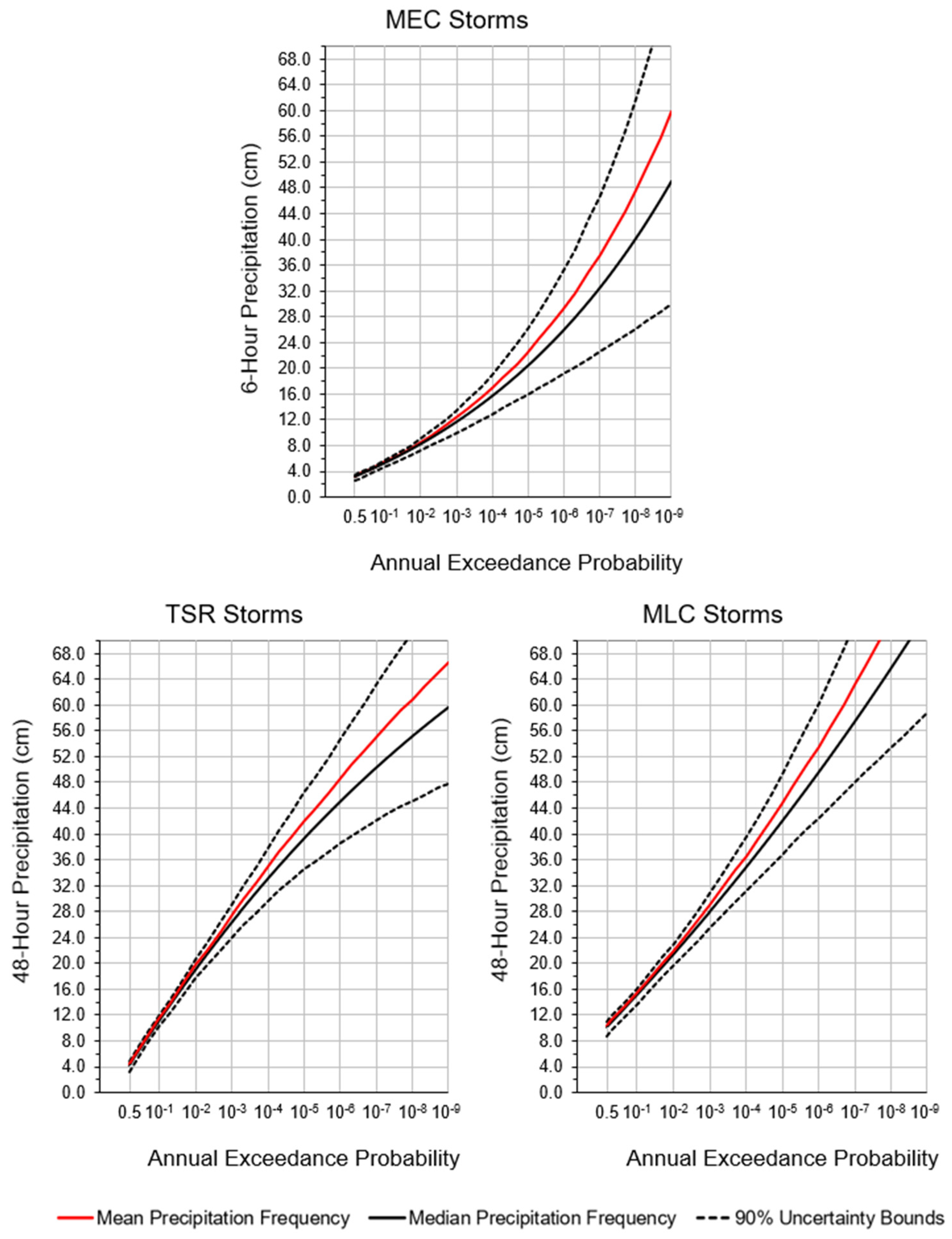
Precipitation frequency relationships define the basin average precipitation depth of a stochastic storm event with a given AEP within the watershed of interest and are developed for each storm type used in the stochastic model. Similar to the development of storm templates described in Section 2.2.2, precipitation frequency relationships from data referenced in the SDTT are developed according to the isopercental analysis methodology [31,32], along with a regional L-moment analysis of storm type and duration [33]. For the combined watershed of Dam A, Dam B, and Dam C, regional probability distributions for key storm durations characterize uncertainty and are developed from historical records, point to area relationships, multiple linear regression, and Thiessen polygon analyses. For MLC and TSR storms, a 48 h precipitation is computed on the watershed level. Precipitation annual maxima for a given station within a watershed can vary from a wide range of storm patterns and storm magnitudes for MEC storms. Thus, the watershed raster is randomly placed relative to the fixed precipitation raster field according to the spatial behavior of historical storms, and a 6 h duration is chosen as the key duration representative of the time during which most of the precipitation occurs [34,35]. The precipitation frequency relationship is shown to have a strong influence on flood frequency estimation for extreme events, making it paramount to develop accurate relationships for the watershed being studied [4,36].
The resulting precipitation frequency relationships for a range of percentiles from the 5th to the 95th are shown in Figure 3. The mean curve is calculated as the expected value of the percentiles. A precipitation frequency areal reduction factor (PFARF) is used to relate the median point precipitation frequency curve to the areal average precipitation frequency data, and percentile results are related to the median by scaling factors. PFARFs and scaling factors are obtained by interpolating the results of stochastic storm generation studies at other watersheds across the Tennessee Valley region [35].

2.2.4. Initial Conditions from Long-Term Simulation

A long-term simulation of synthetic hydrology is completed to establish initial watershed conditions for the stochastic events. Synthetic hydrology is a dataset constructed by resampling statistical distributions of historical mean areal precipitation data for every sub-basin in the Tennessee Valley and synthesizing alternating wet and dry events into a time series of 1000 years of continuous hydrology. By resampling precipitation from the sub-basin statistical distribution rather than actual observed events, the long-term hydrology reflects historical trends but better captures the statistical tails of the rainfall distribution. These synthetic hydrology data are used as input to the Sacramento soil moisture accounting (SAC-SMA) and unit hydrograph models [37]. The SAC-SMA and unit hydrograph models produce continuous flows and sub-basin outlets, which are then provided to RiverWare (a river and reservoir modeling tool offered by CADSWES to simulate reservoir system operations) [38]. The simulated reservoir responses, soil moisture states, and river states make up the initial conditions associated with a sampled date from the long-term simulation.

2.3. Stochastic Calculations

Once the necessary inputs and initial conditions are obtained, they are sampled within each stochastic simulation to define initial watershed conditions and storm characteristics. For each stochastic event simulation, a synthetic precipitation event is inserted within the context of the continuous precipitation time series from the long-term simulation according to the following steps:
  • Sample precipitation depth: the watershed precipitation frequency curve is used to sample the precipitation depth at the key duration of the specified storm type (e.g., 48 h for MLC and TSR, 6 h for MEC).
  • Sample storm template: The spatial and temporal distribution of the storm is determined by sampling from the available set of storm templates. An AEP range limits when a storm template may be selected based on the probability of the sampled rainfall event.
  • Scale the storm template: the selected storm template is then scaled such that the average storm depth across the watershed is equal to the depth of precipitation sampled from the precipitation frequency curve.
  • Sample date from long-term simulation: a date is randomly sampled from the long-term simulation in accordance with the seasonality of the storm type under consideration and is used to set the initial conditions for the stochastic event and define its placement within the overall precipitation time series.
  • Insert stochastic event: MLC, MEC, and TSR storms are inserted within the context of the continuous precipitation time series from the long-term simulation. A dry period of 48 h is maintained before and after MLC and TSR events. Three sub-types of MEC storms (isolated, multi-day, and hybrid) are defined based on the precipitation surrounding an MEC event (MEC events may be embedded within other storms). The sampling algorithm considers the appropriate type of MEC storm to insert on a given date and the probability associated with the given sub-type in each season.
  • Execute stochastic event simulation and compute statistics: After establishing the precipitation sequence and initial conditions, watershed and operational models can be executed to route the stochastic event. The output statistics from watershed models (e.g., peak headwater, peak discharge) are collected and used in the analysis of hydrologic hazards and creation of hydrologic hazard curves.

2.3.1. Stratified Sampling and Convergence

A stratified sampling technique is employed, allowing storm depths and templates to be selected strategically based on defined AEP levels that will be influential in the development of hydrologic hazard curves. Using Neyman’s [39] optimal sample allocation method, precipitation depths are categorized in 100 bins that span the total sampled AEP range for precipitation depths. A fixed number of samples are drawn from each bin and used as inputs for the stochastic calculation procedure defined above in Section 2.3. The probability of exceeding a specific threshold (such as peak headwater or flow) by sampling within a precipitation bin is calculated empirically as the ratio of the number of outputs exceeding a threshold to the total number of samples drawn from the given bin. Key hydrologic hazard metrics are computed for each simulation and used in developing annual exceedance probability curves according to the total probability theorem as follows [40,41,42,43]:
p Q q = i p i w i
where p Q q = probability that Q exceeds a threshold q (i.e., the annual exceedance probability); Q = value of hydrologic hazard response variable of interest (e.g., reservoir inflow, peak discharge); q = specified threshold of the hydrologic hazard response variable Q ; p i = C o u n t   Q n   q / N = probability that Q exceeds the threshold q within the precipitation bin; w i = incremental probability (width) of the precipitation bin; i = index identifying the sampled precipitation bin; n = index identifying the nth simulation output for the hydrologic response variable within a given bin; and N = total number of samples from a given bin.
Bins containing rarer precipitation events are “larger” in that they will be sampled more frequently to gain results applicable to more extreme thresholds of interest. Depending on the threshold of interest, selective sampling can be made from precipitation bins (which will influence overall results), while precipitation bins that will not influence results can be excluded. A breakpoint is defined for a given threshold of interest such that no sampling is conducted in bins below a certain AEP, but all bins that could influence results are included in sampling. This allows for reduced computation time by limiting the number of required simulations.
A two-sided confidence interval is computed to determine when sufficient sampling has been completed for the estimation of a given hydrologic hazard variable. The Clopper–Pearson confidence interval is used to compute the two-sided 90-percent confidence interval for a specific threshold of a variable of interest [44]. The width of the confidence interval is assessed and required to be within a user-defined percentage of the corresponding AEP value of the output variable. Samples are incrementally added per precipitation bin until the confidence interval sufficiently converges for a computed AEP value, signifying that additional sampling would have minimal impact on the resulting hydrologic hazard curve.

2.4. Stochastic Model Calibration

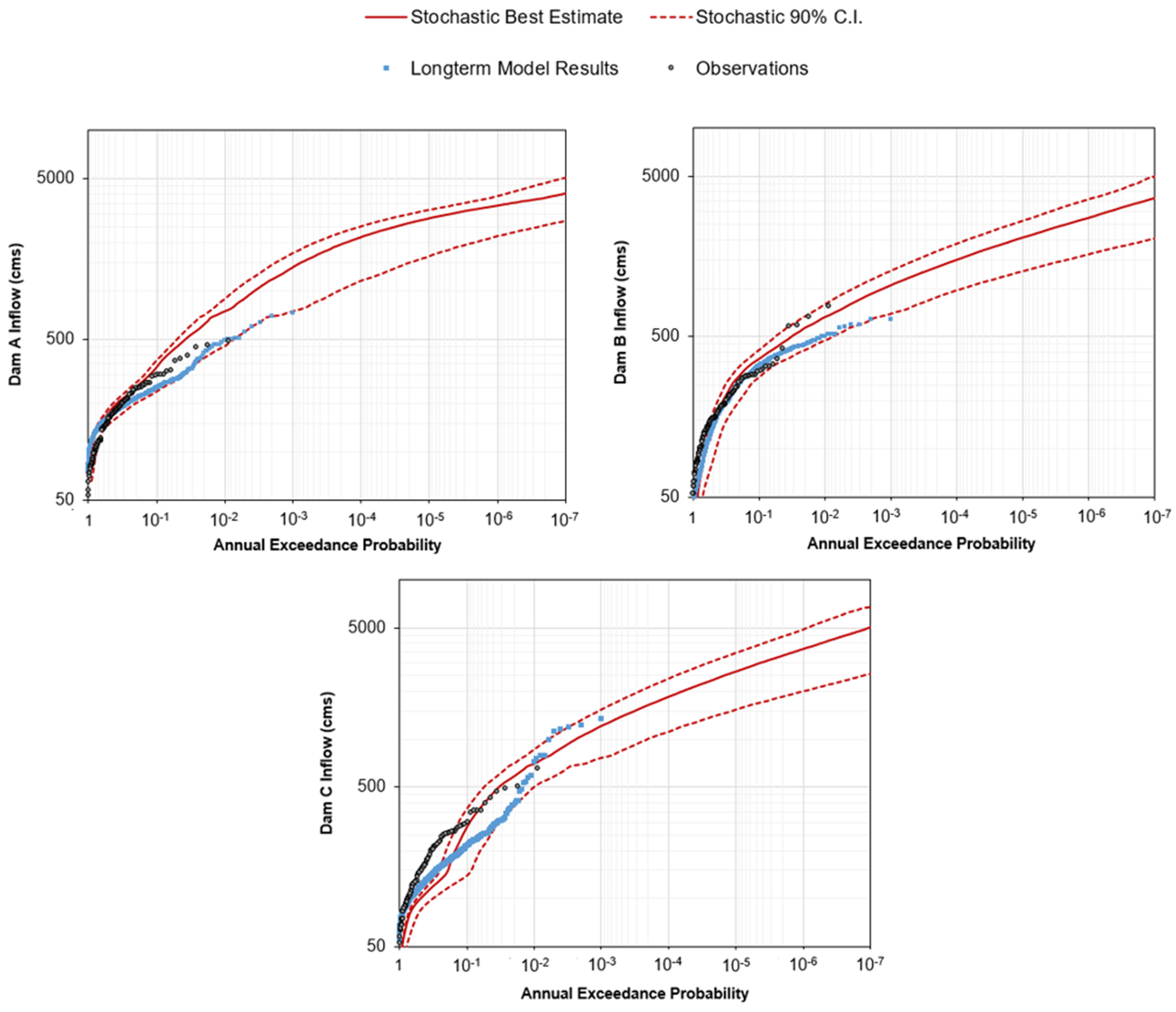
Reservoir inflow during large storm events is a key parameter that directly influences the hydrologic loading placed on a dam [1]. Thus, it is critical to ensure that inflow volumes simulated through stochastic modeling accurately represent the prevailing hydrologic regime and reservoir operations. The watershed model must be able to accurately simulate reservoir inflow to ensure that the consumption of controllable storage during a storm event is modeled appropriately. To ensure proper calibration of the SEFM results, estimated historical annual peak inflows for the studied reservoirs and the results from the 1000-year long-term simulation are compared with the stochastic simulations, as shown in Figure 4. The estimated local inflow data are TVA’s best estimate of inflows compiled from several data sources, including reverse routing and gage scaling.
Simulated annual peak inflows from the long-term simulation tend to be lower than estimated historical annual peak inflows for probabilities ranging from 0.01 to 0.001; however, the stochastic simulation captures both data sets within the 90% confidence interval for the majority of data points and shows a general agreement with the data trends. Of most importance is the ability to model inflow volumes for the extreme storms beyond an AEP of 0.001 to supplement the historical dataset. The results indicate that the stochastic simulations sufficiently characterize inflow for rare events within the range of confidence.

2.5. Empirical Method to Determine Bivariate Exceedance Probabilities

An empirical methodology is developed to expand the stratified sampling technique outlined in Section 2.3.1 to allow for the determination of a bivariate probability distribution. In this methodology, spillway discharge is assessed at any two of the studied dams during individual stochastic events to determine the probability that a pair of spillway discharges would exceed a defined threshold at each dam. Spillway discharge pairs for the studied dams are obtained for a single sampled storm event within a given precipitation bin. The process of empirically determining the annual exceedance probability is then carried out as in Equation (1) but modified to account for a second hydrologic variable (i.e., spillway discharge at a second dam). This results in annual exceedance probabilities being described as a probability surface representing the likelihood of discharge pairs at the selected dams, defined as:
Q A q A ,   Q B q B = i P i w i
where p Q A q A ,   Q B q B = probability that Q A exceeds the threshold q A and Q B exceeds the threshold q B ; Q A , Q B = value of hydrologic hazard response variable of interest for a given dam (e.g., spillway discharge at Dam A, B, or C); q A , q B = specified threshold of the hydrologic hazard response variable Q at a given dam; P i = C o u n t   Q A n   q A , Q B n   q B / N = probability that Q A exceeds the threshold q A and Q B exceeds the threshold q B within the precipitation bin; w i = incremental probability (width) of the precipitation bin; i = index identifying the sampled precipitation bin; n = index identifying the nth simulation output for the hydrologic response variable within a given bin; and N = total number of samples from a given bin. Resulting probability surfaces are shown in Section 3.2.1.

2.6. Calculation of Bivariate Empirical Failure Probability

Bivariate exceedance probabilities for spillway discharge pairs are used to determine the probability of simultaneous dam failures in response to a simulated storm event. Spillway fragility curves for the studied dams are used to associate the hydrologic loading from spillway discharges with probabilities of spillway failure (see Section 2.6.1). A conditional probability relationship is developed to describe the interaction between hydrologic loading and failure probability, and defined as:
p ( F A , F B ) = p Q A q A ,   Q B q B × F A q A ) × p ( F B | q B )
where p ( F A , F B ) = probability that spillway discharge leads to failure at two specified dams during the same storm event (e.g., Dam A, B, or C); p Q A q A ,   Q B q B = probability that Q A exceeds the threshold q A and Q B exceeds the threshold q B ; Q A , Q B = value of hydrologic hazard response variable of interest for a given dam (e.g., spillway discharge at Dam A, B, or C); q A , q B   = specified threshold of the hydrologic hazard response variable Q at a given dam; and p F A q A ) ,   p ( F B | q B ) = probability of spillway failure given that a discharge threshold has been met. Resulting probability surfaces are shown in Section 3.2.2.

2.6.1. Failure Estimate from Generalized Spillway Fragility Curves

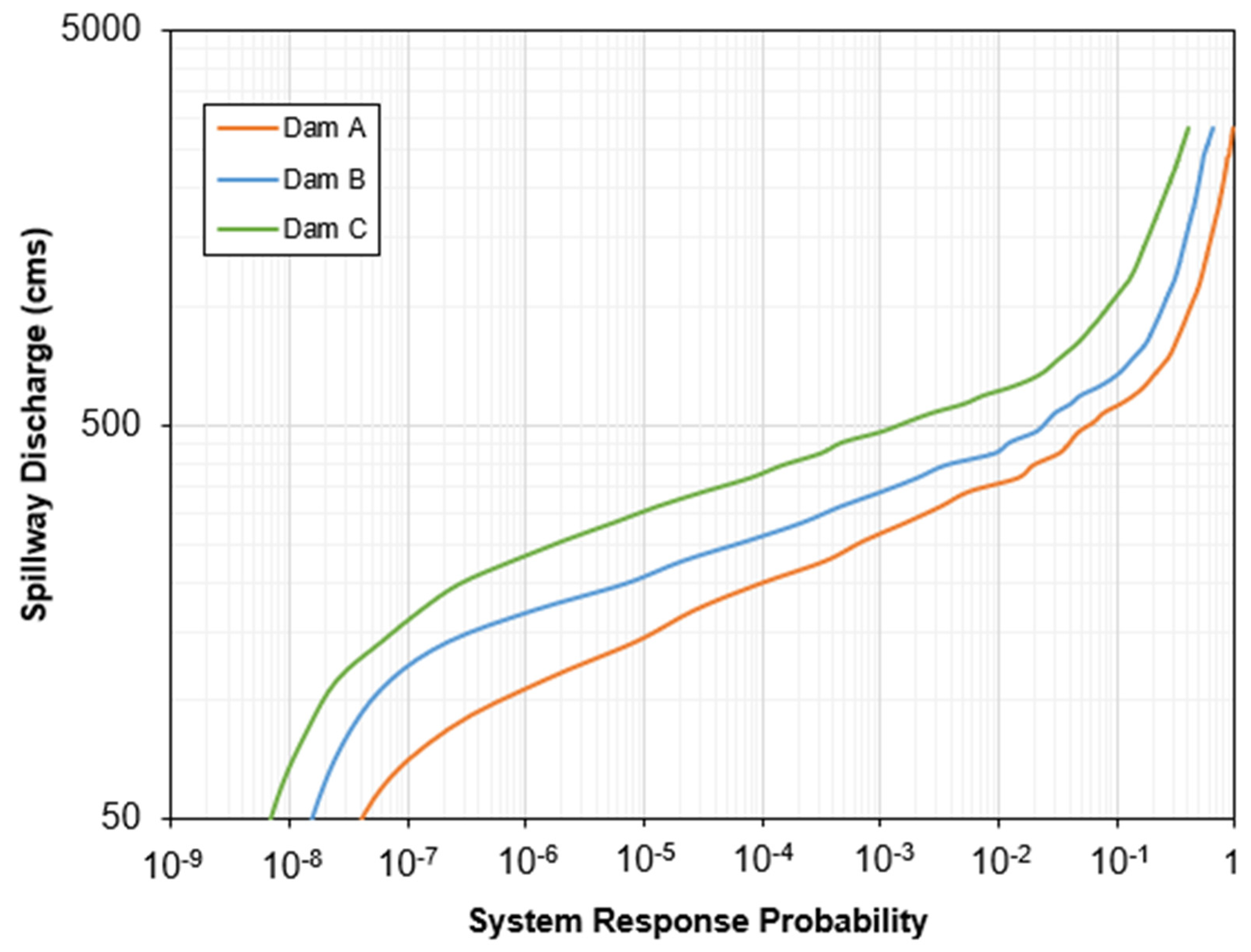
Generalized spillway fragility curves shown in Figure 5 are used to determine the probability that a given hydrologic loading would result in spillway failure (termed the system response probability) for the evaluation of Equation (3). The term failure is used here to refer to any situation in which the hydrologic loading causes damage to the spillway which progresses to a breach and uncontrolled release of the reservoir. The hypothetical spillway fragility curves presented here are informed by general knowledge of the spillways so that the values of the generalized curves would yield realistic results based on end behavior and rates of change with increasing discharge; however, the actual values presented here do not reflect the expected failure probabilities of the studied dams or the relative magnitudes of failure across the dams. Patterns of failure response based on dam combinations, correlation of stochastic simulation results, and relative differences between system and individual risk are preserved here to demonstrate applied methodology and the significance of results.

3. Results

3.1. Assessment of Discharge Correlation

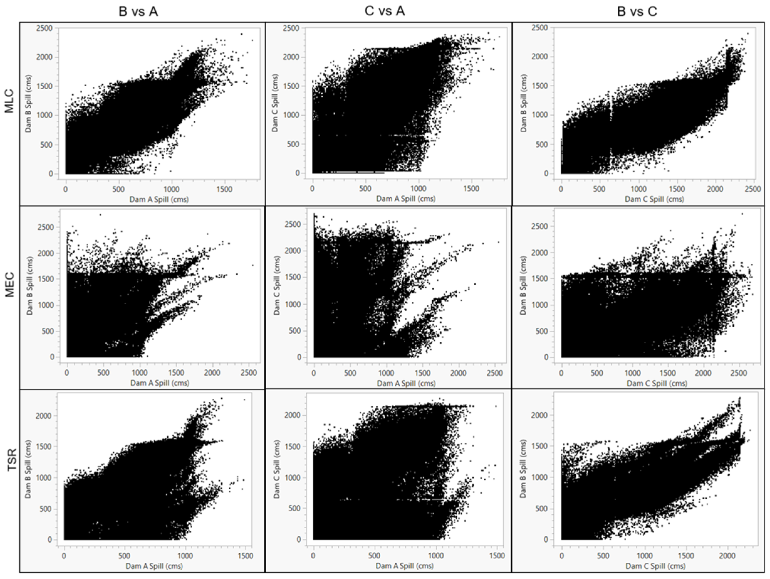
Stochastic simulation results were analyzed with the goal of determining the probability of coincident dam failures due to spillway discharges resulting from a sampled storm event. The dependence of spillway discharge values between selected dams was ascertained using Pearson’s linear correlation coefficient, as shown in Figure 6 and Table 1. A bivariate approach was chosen, allowing for the comparison of two dams at a time as opposed to assessing all three dams simultaneously. This approach allowed for easier processing, visualization, and interpretation of results and the assessment of the more likely case of two dams failing versus three. Confirmation of discharge correlation discussed in Section 4.1 validated further investigation into probabilities associated with spillway discharge pairs.

3.2. Probability Surfaces Based on Dam Combination and Storm Type

3.2.1. Spillway Discharge Pair Exceedance Probability

Probability surfaces describing the empirical bivariate exceedance probabilities for spillway discharge pairs at selected dams for each simulated storm type were calculated as described in Section 2.5 and are shown in Figure 7. As the discharge became greater at each observed dam, the probability of meeting or exceeding the coincident discharge pair became smaller. As shown in Table 1, the MLC and TSR storms demonstrated greater correlation between each of the observed dams when compared with the MEC storms. Thus, it follows that the probability of exceeding most discharge pairs at selected dams would be greater for simulations of MLCs and TSRs than for MECs, as shown in the results.

3.2.2. Joint Failure Probability

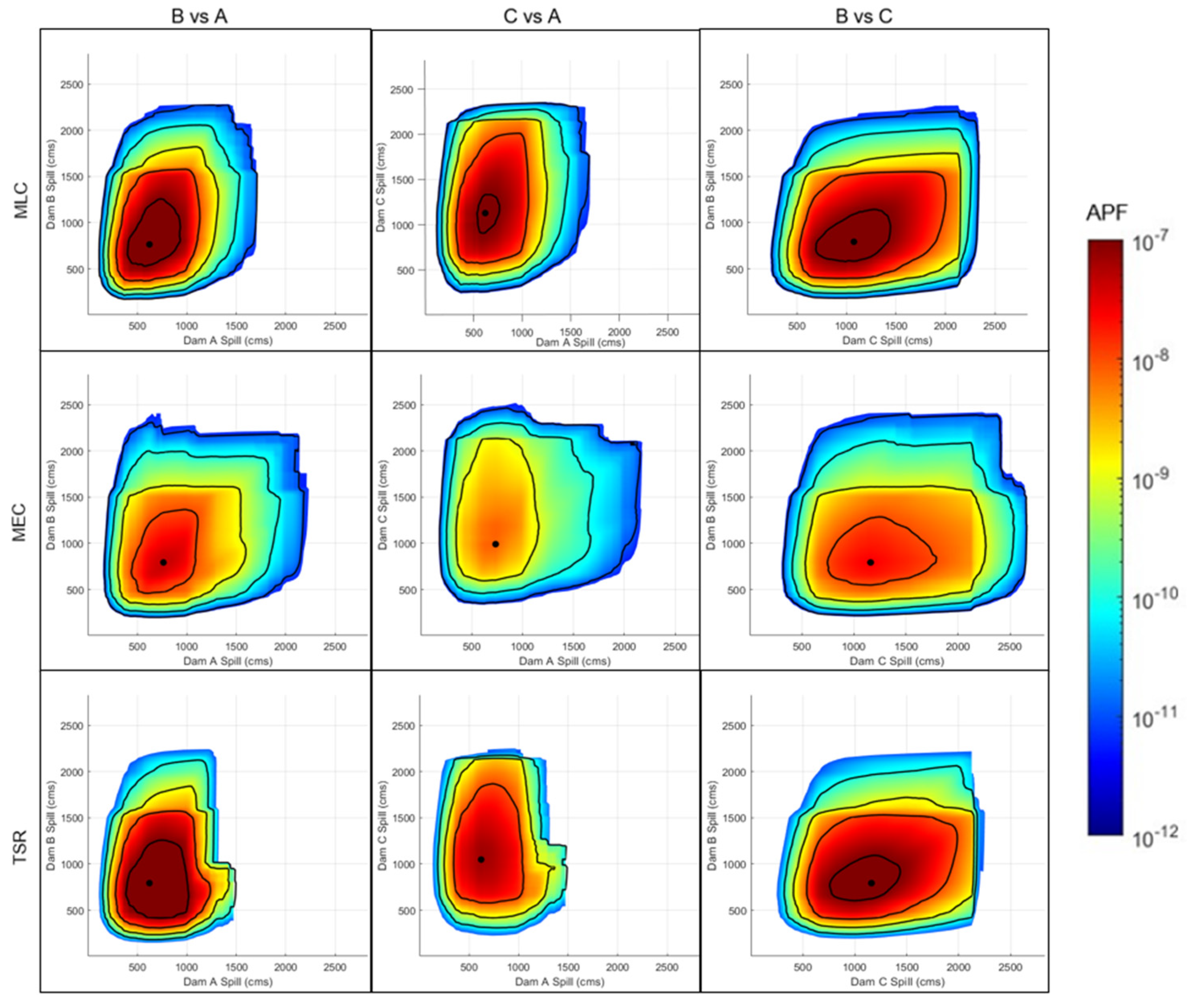
Probability surfaces describing the empirical bivariate failure probabilities for spillway discharge pairs at selected dams for each simulated storm type were calculated as described in Section 2.6 and are shown in Figure 8. According to Equation (3), the hydrologic annual exceedance probabilities associated with each spillway discharge were multiplied by the system response probabilities obtained from the spillway fragility curves for each dam (see Section 2.6.1) to obtain an estimate of annualized probability of failure (APF). The resulting joint failure probability (termed the system failure probability) was plotted as the failure surface according to the combination of observed dams and sampled storm type. Local maxima representing the maximum system failure probabilities for spillway discharge pairs are presented in Table 2.

3.3. Best Estimate of Bivariate and Univariate Failure Probability

To capture the influence of significant storm types encountered in the Tennessee Valley region, this study included stochastic sampling of MEC, MLC, and TSR storms described in Section 2.2.1. Stochastic simulations involving these storm types considered spatial and temporal characteristics that produced a range of flood hydrograph shapes, runoff durations and volumes, and resulting peak discharges. Considering hydrologic hazard curves produced individually by each storm type provided insight into the response of the watershed to specific storm characteristics, but a best estimate of hydrologic hazards was determined by combining the results from the analysis of each storm type to account for the possibility of any storm type occurring in a given year. A total hydrologic hazard curve may be developed to determine the best estimate of hydrologic hazards assuming the independence of the results from each storm type.
Equation (4) was applied to the results for bivariate empirical failure probability for each storm type shown in Figure 8 to yield the best estimate of bivariate system failure probabilities. Similarly, hazard curves for the best estimate of spillway discharge at each individual dam were obtained by applying Equation (4) to the univariate results. System response probabilities from Figure 5 were then sampled and used to scale the best estimate hydrologic hazard curves for spillway discharge at each dam, resulting in univariate failure probabilities in response to spillway discharge. The results of calculating the best estimate for bivariate and univariate system failure probabilities are shown in Table 3 and Figure 9.
B e s t   E s t i m a t e   A E P = 1 1 A E P M E C × 1 A E P M L C × ( 1 A E P T S R )

4. Discussion

4.1. Discharge Correlation

Results from Figure 6 and Table 1 indicate that correlation in regulated spill existed between dams for the storm events sampled, and the correlation varied based on the dams being analyzed and the type of storm used in the stochastic simulations. In agreement with other flood frequency studies, the spatiotemporal characteristics of storms showed a significant influence on maximum flood discharges at the scale of the studied watershed [28,36]. Among the three storm types, the highest correlation and covariance was exhibited by MLC storms, with the lowest being exhibited by MEC storms; moreover, mean peak spillway discharge at each project was the highest for MLC storms and the lowest for MEC storms. The small-scale convective storm patterns that characterized MEC storms led to chaotic spatial distributions of precipitation, reducing the likelihood for loading to be concentrated on a specific area to produce high flows that were correlated at multiple sites. This reaffirms the results of previous studies that indicated that spatial characteristics of storms have significant impact on peak flood discharges for drainage areas of the size studied [28]. MLC and TSR storms, on the other hand, exhibited extended durations of precipitation, gradually varying precipitation gradients, and large total precipitation volumes at low to moderate intensity, resulting in higher average peak spillway discharges, which exhibited significant correlation between dams.
A visual inspection of the bivariate fit plots in Figure 6 further demonstrates the dependence of the resulting spillway discharges on the spatial and temporal characteristics of the different storm types. As noted, the MLC and TSR storms were the most correlated and demonstrated a positive relationship among each dam combination. For each set of simulations, the least correlation was observed for the combination of Dam A and Dam C, a result of these dams being separated by a greater distance than the other dam combinations; however, the larger footprint and gradually varying spatial distribution of MLC and TSR storms allowed some correlation to remain. Several distinct clusters and thresholds may be visually identified for each set of simulations. This behavior was a result of the stochastic sampling procedure. As storm templates and precipitation volumes were selected through Monte Carlo sampling, the distinct spatial and temporal characteristics of specific storm templates caused some results to group together, as similar patterns of hydrologic loading were experienced across the three dams and scaled based on precipitation volume. Similarly, the stochastic sampling may involve repeated simulations of storms that produced a relatively constant discharge at one observed dam and varying discharge at another due to the spatial distribution of rainfall, creating distinct horizontal and vertical lines of grouped discharge values. Although the average peak spillway discharges were the greatest for MLC and TSR storms, MEC storms exhibited the largest maximum spillway discharge pairs of the three storm types. This behavior was likely a result of the high-intensity MEC storms being sampled most often during the summer months when reservoirs were maintained at higher pool levels. The higher starting pool elevation resulted in higher maximum simulated spillway discharge values for a given sampled depth of precipitation.

4.2. Assessment of Discharge and Failure Probabilities

4.2.1. Bivariate Discharge Pair Exceedance Probabilities

From the results shown in Figure 7, the bivariate AEP of 1 in 10,000 years (10−4) resulted from spillway discharge pairs generally in the range of 600–900 cubic meters per second (cms) for MLC and TSR storms, while MEC storms reached this discharge pair threshold around an AEP of 1 in 100,000 years (10−5) or rarer, indicating that it is significantly more likely for MLC and TSR storms to bring about coincident spillway discharges of this magnitude. As discharge pairs became increasingly rare, however, the distinction between storm types and dam combinations became less apparent, as the rarity of the hydrologic loading controlled the probability estimate. This was consistent with studies considering influence factors on spatially distributed stochastic models [28]. For discharges generally beyond the 1 in 1,000,000-year (10−6) return period, MEC storms showed more correlation, as intense precipitation occurred in the summer with the reservoir at a higher pool, leading to more frequent spilling (see Section 4.1). Stochastic sampling of storm types and storm templates resulted in a different range of discharges depending on the observed dam, and, typically, the most extreme storms for each set of simulations appeared in a single precipitation bin. These characteristics of the stochastic sampling led to differing values of maximum spillway discharge pairs among dam combinations and jagged edges at the extremes of the probability plots.

4.2.2. Bivariate Failure Probabilities

System failure probabilities shown in Figure 8 generally became the greatest, in the range of 600 to 1100 cms across all storm types and dam combinations. As shown in Table 1, the MLC and TSR storms demonstrated greater correlation in peak spillway discharge between each of the observed dams when compared with the MEC storms. Thus, it followed that the hydrologic exceedance probability for a given discharge pair and dam combination was roughly one order of magnitude greater for simulations of MLCs and TSRs than for MECs. Moreover, the general shape of the failure surfaces was the most similar between the MLCs and TSRs, as these storm types produced similar correlation in discharge among the dams. However, there were similarities across all storm types considering the range of discharge pairs corresponding to maximum system failure probability and the general slope of each surface associated with a combination of dams. These similarities reflected the influence of the physical characteristics associated with each dam such as relative location, elevation, surrounding topography, and available storage. The hydrologic exceedance probabilities were the controlling factor in determining the maximum system failure probabilities given that they were much rarer than the system response probabilities for the associated discharge pairs. Regardless of the sampled storm type, the combination of Dam A and Dam C had the rarest hydrologic exceedance probability in response to the increased distance between these dams, limiting the likelihood of coincident spillway discharge.

4.2.3. Univariate and Bivariate Best Estimate of Failure Probability

Inspection of the univariate and bivariate failure probabilities in Figure 9 and Table 3 shows that the estimate of joint failure was between three and four orders of magnitude more likely (7.42 × 10² to 5.68 × 10³) when the dependence of spillway discharge between the dams was considered as opposed to assuming the failure of each project resulted from an independent hydrologic event. This was calculated by comparing the joint system failure probabilities (e.g., (A, B)) in Table 3 with the corresponding product of failure probabilities for the individual dams (e.g., A × B). As the best estimate method described in Section 3.3 considered the contributions of each storm type, the best estimate system failure probabilities were slightly greater when compared with the individual storm type results. Inspection of the best estimate surface plots for bivariate failure probability showed that the contributions from the MLCs and TSRs controlled the response at the most common probabilities; however, the best estimate surfaces also considered the impact of the MEC storms, which produced the greatest maximum discharge pairs, as discussed in Section 4.1. As a result, the best estimate curves were able to represent the correlation of MLCs and TSRs caused by the extended durations of precipitation, gradually varying precipitation gradients, and large total precipitation volumes while also accounting for the largest maximum discharge pairs that resulted from MEC storms with intense precipitation pockets during the summer months when the reservoir was at the highest antecedent pool elevations.
As shown in Table 3, bivariate best estimates for maximum system failure probabilities were one to two orders of magnitude rarer than univariate best estimates of maximum system failure probability at each dam. The contribution to increased rarity between the bivariate and univariate case was split between the hydrologic exceedance probability and the system response probability. Inspection of the results shows that the hydrologic exceedance probability and the system response probability were each roughly one order of magnitude rarer in the bivariate case than the univariate case. Thus, similar levels of hydrologic loading were more likely to occur at a single dam than coincidently at a combination of dams, and the risk of a single dam spillway failure in response to such loading was more likely than coincident dam spillway failures.

4.3. Characterization of System Risk

As discussed in Section 2.6.1, the actual magnitude of system failure probabilities will differ depending on the spillway fragility curves referenced to determine system response probabilities. Consequently, the significance of the results from this study should be assessed based on the relative differences between system and individual risk that would not be influenced by system response curves, since the same spillway fragility was applied in both univariate and bivariate cases. Considering the relative difference between system failure probability for bivariate and univariate cases, the results suggest that a coincident failure was between one and two orders of magnitude rarer than a failure at an individual dam.
Although the coincident failure of two dams is up to 100 times less likely to occur than an individual dam failure based on these results, the characterization of the risk associated with coincident failure could still prove significant in relation to the risk associated with an individual failure. Given that risk is characterized by the frequency of hazardous events such as floods and earthquakes, the response of a dam to a hazard (failure mode), and the potential consequences of failure, the occurrence of coincident dam failures could pose significant risk driven by the consequences of multiple dams failing in response to a single storm event [1,8].
To fully consider risk on a system level, additional factors influencing failure modes and failure progression must be considered [1]. Once the hydrologic loading probabilities are determined through the development of hazard curves, there are still many factors related to failure modes and consequences that must be accounted for when determining risk. Additional risk factors include the uncertainty of the failure mechanism itself, the time required for the failure to progress from initiation to full failure, and the impact of detection and intervention. In the case of a system of dams with the potential for coincident failure, the failure progression time for each dam will be critical for the estimation of downstream consequences and emergency response. Considering spillway failure modes such as those hypothesized in this study, the failure progression time at each spillway could result in a range of maximum discharges encountered by downstream communities; moreover, the degree to which failures progress simultaneously will place increased strain on the emergency response staff called upon to intervene and prevent or reduce the consequences of failure.

4.4. Factors Influencing Sensitivity of Stochastic Simulation Results

Similar to the discussion in this study concerning the influence of factors such as storm templates, storm types, initial conditions, and model parameters on the stochastic simulation results (see Section 1.3), other studies have shown that certain factors influence flood frequency estimates with varying levels of sensitivity [45,46]. Essential to the utility of stochastic modeling is the ability to address the assumption of AEP neutrality by assigning probability estimates to hydrologic parameters. The impact of initial conditions, precipitation inputs, and randomly sampled model parameters on flood frequency estimates may be assessed based on the output from a hydrologic model [27]. However, a structured modeling framework with varying parameters and initial conditions can perform differently based on the type of hydrologic event being modeled and the hydroclimate under consideration [47,48]. Therefore, depending on the application, it may be justifiable to use multiple modeling structures for stochastic flood frequency studies to identify or reduce potential variability in results [4]. Moreover, an understanding of the sensitivity of resulting flood frequency estimates in response to varying model inputs may provide a means to reduce uncertainty.

4.4.1. Hydrologic Model Structure

Common hydrologic models, including the Hydrologic Engineering Center hydrologic modeling system (HEC-HMS) and the Sacramento soil moisture accounting (SAC-SMA), are shown to exhibit varying outputs resulting from interactions between model structure and model parameters, particularly for flood metrics involving multi-day volumes; moreover, examination of stochastic flood frequency estimates using these hydrologic models suggests that model structure has a measurable influence on results across return periods at least up to the 100,000-year event [4,37,49]. This highlights the importance of assessing all assumptions underpinning the hydrologic models used within a stochastic modeling framework to best characterize flood generation processes and select models appropriate for the watershed being studied.

4.4.2. Model Inputs

Initial conditions such as soil moisture content can introduce relatively significant variability in flood frequency estimates for more frequent flood events nearing the 1000-year return period, especially in arid environments [50]. As the AEP becomes increasingly rare, precipitation frequency distributions have been shown to have the most influence on stochastic flood modeling with respect to other inputs [4]. Thus, the accuracy of hydrometeorological studies used to develop precipitation frequency estimates is critical for stochastic flood frequency analysis focused on extending hydrologic hazard curves to characterize rare events.

4.5. Future Work and Applications

Hydrometeorological inputs are an essential component of stochastic models used to develop hydrologic hazard curves, and studies that involve data collection, data quality control, and the extension of historical records are essential to improving the accuracy of flood frequency estimates [1]. However, as discussed in Section 4.4, there is varying sensitivity of flood frequency estimates in response to hydrometeorological inputs such as precipitation frequency relationships. Given that the precipitation frequency relationships for a watershed are a dominant factor in determining flood frequency of extreme events, further study into the influence of the spatial representation of watersheds and the spatial and temporal variability of rainfall on flood frequency estimates could have an impact on modeling approach and interpretation of results [28,51]. Moreover, if flood frequency results are to be compared between different watersheds to assess the impact of different storm types or operation policies on hydrologic response at multiple projects, either consistent methodologies for determining flood frequency will need to be used or differences in methodology will need to be quantified [4]. Comparison within the Tennessee Valley watershed is made possible by consistent meteorological studies and scaling procedures across the entire region, and similar actions could be taken in other regions where there is a desire to compare watershed responses to obtain consistent measures of flood frequency and hydrologic risk.
Stratified sampling and convergence methods developed according to the total probability theorem could be extended to evaluate exceedance probabilities for discharge thresholds at three or more dams rather than focusing on two dams, as occurred in this study [40]. Further investigation into the joint exceedance probabilities and failure probabilities of groups of closely related dams could provide valuable information for risk studies. It is expected that, as is shown in this study, the probability of coincident failure for a group of dams will be less likely than individual failures; however, the consequences associated with coincident failures may be significant and require consideration within risk reduction measures. Continued study into the dynamic interaction between systems of dams acting in parallel could lead to new discoveries related to operation policy and best practices for managing large flood events. Similar analyses could also be applied to dams in series, with outflows from one dam directly influencing inflows to another.

5. Conclusions

In support of the continued integration of risk-informed decision making and the expanded use of PFHA for hydrologic hazard studies at dams, this study accomplished the objectives of (a) assessing the correlation of peak spillway discharges across three dams in adjacent similarly sized watersheds; (b) determining hydrologic exceedance probabilities for spillway discharge pairs at selected dams in response to MLC, MEC, and TSR storm types; and (c) calculating the probability of coincident dam failures to characterize risk posed by a system of dams in addition to risk posed by an individual dam.
Correlation of stochastic simulation results, patterns of failure response based on dam combinations, and relative differences between system and individual risk were examined using generalized spillway fragility curves, as discussed in Section 2.6.1. A pattern of correlation in spillway discharge was observed between dams for the storm events sampled, with the correlation varied based on the combination of dams and the type of storm used in the stochastic simulations. Dam and storm type combinations that exhibited the greatest correlation in average peak spillway discharges also exhibited the greatest hydrologic exceedance probabilities and, consequently, the greatest joint failure probabilities. Results from Section 3.3 show that the estimate of joint failure was three to four orders of magnitude more likely (7.42 × 10² to 5.68 × 10³) when the dependence of spillway discharge between the dams was considered using the methods of this study as opposed to assuming the failure of each project resulted from an independent hydrologic event.
Future work must address the influence of the spatial representation of watersheds and the spatial and temporal variability of rainfall on flood frequency estimates. These factors could have a significant impact on the stochastic modeling approach and interpretation of results [28,51]. There is a need to better understand the dynamic interaction between systems of dams acting in parallel. Similar to research conducted on dams in series, interconnected system components such as initial reservoir levels, storage availability, and reservoir operations and discharge capabilities may have a more significant impact on overtopping and failure probabilities than inflows [7]. An increased understanding of the response of a system of dams to extreme storm events could better inform reservoir storage regulation policies and provide increased resiliency in response to weather variability and climate change.

Author Contributions

M.G.M. contributed to conceptualization, methodology, analysis, and writing of the original draft preparation; M.B.Y. contributed to conceptualization, methodology, and writing—review and editing of manuscript draft; and J.S.S. contributed to methodology and writing—review and editing of manuscript draft. All authors have read and agreed to the published version of the manuscript.

Funding

This research received no external funding. Research supported through internal funding from the Tennessee River Authority, and the Tennessee Water Resources Research Center through the US Geological Survey 104b Program.

Data Availability Statement

All data produced in this study along with model inflow calibration data are available in the following repository (HydroShare). This dataset includes all stochastically generated flow data from the TVA probabilistic flood hazard analysis (PFHA) framework necessary to reproduce the study results, as well as all MatLab scripts used to process the data in this study. As identified in the data repository, figures in this report were created using JMP Pro 16 and MATLAB R2022b [52,53]. Additional input data for the storm database and transposition tool (SDTT), TVA RiverWare model, and TVA PFHA framework are not openly accessible to the public or research community. These data are considered sensitive due to their connection with critical infrastructure and proprietary software frameworks.

Acknowledgments

A special thanks is extended to the entire team that contributed to the completion of this research project. Those from TVA who provided guidance and critical feedback on manuscript drafts include Patrick Massey, Amanda Turk, and Matthew Williams. Other valuable contributors to the project include Ed Roush (Infisys) and Jonny McIntosh (Research Triangle Institute) for continued support in the development of the TVA PFHA framework.

Conflicts of Interest

The authors declare no conflicts of interest.

References

  1. Smith, C.H.; Bartles, M.; Fleming, M. Hydrologic Hazard Methodology for Semi-Quantitative Risk Assessments: An Inflow Volume-Based Approach to Estimating Stage-Frequency for Dams. In USACE RMC-TR-2018-03; United States Army Corps of Engineers: Washington, DC, USA, 2018. [Google Scholar]
  2. Fleming, M.J.; Duren, A. Stochastic Hydrologic Simulation for Extension of Reservoir Pool Stage Frequency Curves. In Proceedings of the World Environmental and Water Resources Congress, Austin, TX, USA, 17–21 May 2015. [Google Scholar] [CrossRef]
  3. England, J.F., Jr.; Cohn, T.A.; Faber, B.A.; Stedinger, J.R.; Thomas, W.O., Jr.; Veilleux, A.G.; Kiang, J.E.; Mason, R.R., Jr. Guidelines for Determining Flood Flow Frequency—Bulletin 17C. U.S. Geological Survey Techniques and Methods, 2018, Book 4, Chap. B5, 148. Available online: https://pubs.usgs.gov/tm/04/b05/tm4b5.pdf (accessed on 1 October 2022).
  4. Newman, A.J.; Stone, A.G.; Saharia, M.; Holman, K.D.; Addor, N.; Clark, M.P. Identifying sensitivities in flood frequency analyses using a stochastic hydrologic modeling system. Hydrol. Earth Syst. Sci. 2021, 25, 5603–5621. [Google Scholar] [CrossRef]
  5. Zhang, L.; Singh, V.P. Bivariate Flood Frequency Analysis Using the Copula Method. J. Hydrol. Engr. 2006, 11, 150–164. [Google Scholar] [CrossRef]
  6. Requena, A.I.; Mediero, L.; Garrote, L. A bivariate return period based on copulas for hydrologic dam design: Accounting for reservoir routing in risk estimation. Hydrol. Earth Syst. Sci. 2013, 17, 3023–3038. [Google Scholar] [CrossRef]
  7. Micovic, Z.; Hartford, D.N.D.; Schaefer, M.G.; Barker, B.L. A non-traditional approach to the analysis of flood hazard for dams. Stoch. Environ. Res. Risk Assess. 2016, 30, 559–581. [Google Scholar] [CrossRef]
  8. Donnelly, C.R.; Acharya, A.M. A Discussion on the Evolution and Application of Quantitative Risk Informed Dam Safety Decision Making. In ICDSME 2019. Water Resources Development and Management; Mohd Sidek, L., Salih, G., Boosroh, M., Eds.; Springer: Singapore, 2020. [Google Scholar] [CrossRef]
  9. U.S. Water Resources Council. A Uniform Technique for Determining Flood Flow Frequencies, 1967. Technical Bulletin No. 15. U.S. Water Resources Council, Subcommittee on Hydrology, Washington, DC. Available online: https://water.usgs.gov/osw/bulletin17b/Bulletin_15_1967.pdf (accessed on 1 October 2022).
  10. Interagency Committee on Water Data. Guidelines for Determining Flood Flow Frequency, Technical Report Bulletin 17B: 1982. Interagency Committee on Water Data, Hydrology Subcommittee. Available online: https://relicensing.pcwa.net/documents/Library/PCWA-L%20465.pdf (accessed on 1 October 2022).
  11. Thomas, W.O. A uniform technique for flood frequency analysis. J. Water Resour. Plan. Manag. 1985, 111, 321–337. [Google Scholar] [CrossRef]
  12. Griffis, V.W.; Stedinger, J.R. Evolution of flood frequency analysis with Bulletin 17. J. Hydrol. Eng. 2007, 12, 283–297. [Google Scholar] [CrossRef]
  13. Cohn, T.A.; England, J.F.; Berenbrock, C.E.; Mason, R.R.; Stedinger, J.R.; Lamontagne, J.R. A generalized Grubbs-Beck test statistic for detecting multiple potentially influential low outliers in flood series. Water Resour. Res. 2013, 49, 5047–5058. [Google Scholar] [CrossRef]
  14. National Research Council. Estimating Probabilities of Extreme Floods: Methods and Recommended Research; National Academy Press: Washington, DC, USA, 1988. [Google Scholar] [CrossRef]
  15. Packman, J.; Kidd, C. A logical approach to the design storm concept. Water Resour. Res. 1980, 16, 994–1000. [Google Scholar] [CrossRef]
  16. Wright, D.B.; Yu, G.; England, J.F. Six decades of rainfall and flood frequency analysis using stochastic storm transposition: Review, progress, and prospects. J. Hydrol. 2020, 585, 124816. [Google Scholar] [CrossRef]
  17. Wright, D.B.; Smith, J.A.; Baeck, M.L. Flood frequency analysis using radar rainfall fields and stochastic storm transposition. Water Resour. Res. 2014, 50, 1592–1615. [Google Scholar] [CrossRef]
  18. Schaefer, M.G.; Barker, B.L. Stochastic Event Flood Model (SEFM). In Mathematical Models of Small Watershed Hydrology and Applications; Singh, V.J., Frevert, D.K., Eds.; Water Resources Publications LLC.: Littleton, CO, USA, 2002; Section 5; pp. 705–745. ISBN 1-887201-35-1. Available online: https://www.cabdirect.org/cabdirect/abstract/20033121363 (accessed on 1 October 2022).
  19. England, J.E., Jr.; Godaire, J.E.; Klinger, R.E.; Bauer, T.R.; Julien, P.Y. Paleohydrologic bounds and extreme flood frequency of the Upper Arkansas River, Colorado, USA. Geomorphology 2010, 124, 1–16. [Google Scholar] [CrossRef]
  20. Paquet, E.; Garavaglia, F.; Garçon, R.; Gailhard, J. The SCHADEX method: A semi-continuous rainfall–runoff simulation for extreme flood estimation. J. Hydrol. 2013, 495, 23–37. [Google Scholar] [CrossRef]
  21. Sharma, A.; Wasko, C.; Lettenmaier, D.P. If precipitation extremes are increasing, why aren’t floods? Water Resour. Res. 2018, 54, 8545–8551. [Google Scholar] [CrossRef]
  22. Nuswantoro, R.; Diermanse, F.; Molkenthin, F. Probabilistic flood hazard maps for Jakarta. J. Flood Risk Manag. 2016, 9, 105–124. [Google Scholar] [CrossRef]
  23. Wing, O.E.J.; Quinn, N.; Bates, P.D.; Neal, J.C.; Smith, A.M.; Sampson, C.C.; Coxon, G.; Yamazaki, D.; Sutanudjaja, E.H.; Alfieri, L. Toward global stochastic river flood modeling. Water Resour. Res. 2020, 56, e2020WR027692. [Google Scholar] [CrossRef]
  24. Schaefer, M.G.; Barker, B.L. Stochastic Event Flood Model (SEFM) User’s Manual; MGS Engineering Consultants, Inc. & MGS Software LLC.: Olympia WA, USA, 2017; Available online: https://mgsengr.com/wp-content/download/SEFM_TechnicalSupportManual_March2018.pdf (accessed on 1 October 2022).
  25. Steinschneider, S.; Brown, C. A semiparametric multivariate, multi-site weather generator with low-frequency variability for use in climate risk assessments. Water Resour. Res. 2013, 49, 7205–7220. [Google Scholar] [CrossRef]
  26. Diermanse, F.L.M.; Carroll, D.G.; Beckers, J.V.L.; Ayre, R.; Schuurmans, J.M. A Monte Carlo Framework for the Brisbane River Catchment Flood Study. In Proceedings of the HWRS Conference, Perth, Australia, 24–27 February 2014; Available online: https://search.informit.org/doi/10.3316/informit.386923464782388 (accessed on 1 October 2022).
  27. Rahman, A.; Weinmann, P.E.; Hoang, T.M.T.; Laurenson, E.M. Monte Carlo simulation of flood frequency curves from rainfall. J. Hydrol. 2002, 256, 196–210. [Google Scholar] [CrossRef]
  28. Zhu, Z.; Wright, D.B.; Yu, G. The impact of rainfall space-time structure in flood frequency analysis. Water Resour. Res. 2018, 54, 8983–8998. [Google Scholar] [CrossRef]
  29. Hunter, R.D.; Meentemeyer, R.K. Climatologically aided mapping of daily precipitation and temperature. J. Appl. Meteor. Climatol. 2005, 44, 1501–1510. [Google Scholar] [CrossRef]
  30. Lobligeois, F.; Andréassian, V.; Perrin, C.; Tabary, P.; Loumagne, C. When does higher spatial resolution rainfall information improve streamflow simulation? An evaluation using 3620 flood events. Hydrol. Earth Syst. Sci. 2014, 18, 575–594. [Google Scholar] [CrossRef]
  31. Shaw, E.M.; Beven, K.J.; Chappell, N.A.; Lamb, R. Hydrology in Practice, 4th ed.; Spon Press: New York, NY, USA, 2011. [Google Scholar]
  32. Micovic, Z.; Schaefer, M.G.; Taylor, G.H. Uncertainty analysis for Probable Maximum Precipitation estimates. J. Hydrol. 2015, 521, 360–373. [Google Scholar] [CrossRef]
  33. Hosking, J.R.M.; Wallis, J.R. Regional Frequency Analysis—An Approach Based on L-Moments; Cambridge Press: Cambridge, UK, 1997; Available online: https://ui.adsabs.harvard.edu/abs/1997rfa..book.....H/abstract (accessed on 1 October 2022).
  34. Schaefer, M.G.; Barker, B.L. Stochastic Modeling of Extreme Floods on the American River at Folsom Dam: Flood-Frequency Curve Extension; US Army Corps of Engineers, Hydrologic Engineering Center: Davis, CA, USA, 2005. Available online: https://www.hec.usace.army.mil/publications/ResearchDocuments/RD-48.pdf (accessed on 1 October 2022).
  35. MGS Engineering Consultants, MetStat, Applied Climate Services, & Riverside Technology. Regional PF Analyses for Mid-Latitude Cyclones, Mesoscale Storms with Embedded Convection, Local Storms and Tropical Storm Remnant Storm Types in the Tennessee Valley Watershed, Prepared for Tennessee Valley Authority. 2015. Available online: https://mgsengr.com/wp-content/download/SimplifiedSEFM_Guidance_20220527.pdf (accessed on 1 October 2022).
  36. Peleg, N.; Blumensaat, F.; Molnar, P.; Fatichi, S.; Burlando, P. Partitioning the impacts of spatial and climatological rainfall variability in urban drainage modeling. Hydrol. Earth Syst. Sci. 2017, 21, 1559–1572. [Google Scholar] [CrossRef]
  37. Bennett, T.H. Development and Application of a Continuous Soil Moisture Accounting Algorithm for the Hydrologic Engineering Center Hydrologic Modeling System (HEC-HMS); University of California: Davis, CA, USA, 1998. [Google Scholar]
  38. Zagona, E.A.; Fulp, T.J.; Shane, R.; Magee, T.; Goranflo, H.M. RiverWare: A generalized tool for complex reservoir system modeling. J. Am. Water Resour. Assoc. 2001, 37, 913–929. [Google Scholar] [CrossRef]
  39. Neyman, J. On the two different aspects of the representative method: The method of stratified sampling and the method of purposive selection. J. R. Stat. Soc. 1934, 97, 558–625. [Google Scholar] [CrossRef]
  40. Benjamin, J.R.; Cornell, C.A. Probability and Statistics for Civil Engineers; McGraw-Hill: New York, NY, USA, 1970. [Google Scholar]
  41. Kuczera, G. Combining site-specific and regional information an empirical Bayes approach. Water Resour. Res. 1982, 18, 306–314. [Google Scholar] [CrossRef]
  42. Nathan, R.J.; Weinmann, E.M.; Hill, P. Use of Monte Carlo Simulation to Estimate the Expected Probability of Large to Extreme Floods. In Proceedings of the 28th International Hydrology and Water Resources Symposium, Wollongong, NSW, Australia, 10–14 November 2003; The Institution of Engineers: Australian Capital Territory, Australia, 2003. Available online: https://search.informit.org/doi/10.3316/informit.350910043129567 (accessed on 1 October 2022).
  43. Tijms, H.C. A First Course in Stochastic Models; John Wiley and Sons: West Sussex, UK, 2003; ISBN 13 978 0471498803. [Google Scholar]
  44. Korn, E.I.; Graubard, B.I. Confidence intervals for proportions with small expected number of positive counts estimated from survey data. Surv. Methodol. 1998, 24, 193–201. [Google Scholar]
  45. Newman, A.J.; Mizukami, N.; Clark, M.P.; Wood, A.W.; Nijssen, B.; Nearing, G. Benchmarking of a physically based hydrologic model. J. Hydrometeorol. 2017, 18, 2215–2225. [Google Scholar] [CrossRef]
  46. Clark, M.P.; Slater, A.G.; Rupp, D.E.; Woods, R.A.; Vrugt, J.A.; Gupta, H.V.; Wagener, T.; Hay, L.E. Framework for Understanding Structural Errors (FUSE): A modular framework to diagnose differences between hydrological models. Water Resour. Res. 2008, 44, W00B02. [Google Scholar] [CrossRef]
  47. Markstrom, S.L.; Hay, L.E.; Clark, M.P. Towards simplification of hydrologic modeling: Identification of dominant processes. Hydrol. Earth Syst. Sci. 2016, 20, 4655–4671. [Google Scholar] [CrossRef]
  48. Mizukami, N.; Rakovec, O.; Newman, A.J.; Clark, M.P.; Wood, A.W.; Gupta, H.V.; Kumar, R. On the choice of calibration metrics for “high-flow” estimation using hydrologic models. Hydrol. Earth Syst. Sci. 2019, 23, 2601–2614. [Google Scholar] [CrossRef]
  49. Anderson, E.A. Calibration of Conceptual Hydrologic Models for Use in River Forecasting; Office of Hydrologic Development, US National Weather Service: Silver Spring, MD, USA, 2002. Available online: https://www.weather.gov/media/owp/oh/hrl/docs/1_Anderson_CalbManual.pdf (accessed on 1 October 2022).
  50. Yu, G.; Wright, D.B.; Zhu, Z.; Smith, C.; Holman, K.D. Process-based flood frequency analysis in an agricultural watershed exhibiting nonstationary flood seasonality. Hydrol. Earth Syst. Sci. 2019, 23, 2225–2243. [Google Scholar] [CrossRef]
  51. Yakir, H.; Morin, E. Hydrologic response of a semi-arid watershed to spatial and temporal characteristics of convective rain cells. Hydrol. Earth Syst. Sci. 2011, 15, 393–404. [Google Scholar] [CrossRef]
  52. JMP Version Pro 16.0.0, SAS Institute Inc.: Cary, NC, USA,, 2021. Available online: https://www.jmp.com/en_us/software.html(accessed on 1 October 2022).
  53. The MathWorks Inc. MATLAB Version: 9.13.0 (R2022b), The MathWorks Inc.: Natick, MA, USA, 2022. Available online: https://www.mathworks.com(accessed on 1 October 2022).
Figure 1. Overview of the TVA PFHA system framework based on SEFM. Arrows indicate inputs to subsequent steps in the modeling framework.
Water 16 00865 g001
Figure 2. Generalized depiction of watersheds for each studied dam showing watershed characteristics and relative dam locations.
Water 16 00865 g002
Figure 3. Precipitation frequency relationships for mesoscale storms with embedded convection (MEC), mid-latitude cyclone (MLC), and tropical storm remnant (TSR) storm types for stochastic simulations.
Water 16 00865 g003
Figure 4. Calibration of stochastic simulation results considering estimated local flows and 1000-year long-term simulation data.
Water 16 00865 g004
Figure 5. Generalized spillway fragility curves used to simulate system response probabilities.
Water 16 00865 g005
Figure 6. Bivariate fit of spillway discharge data between pairs of dams for embedded convection (MEC), mid-latitude cyclone (MLC), and tropical storm remnant (TSR) storm types.
Water 16 00865 g006
Figure 7. Empirical bivariate exceedance probabilities for spillway discharge pairs at selected dams for the embedded convection (MEC), mid-latitude cyclone (MLC), and tropical storm remnant (TSR) storm types.
Water 16 00865 g007
Figure 8. Empirical bivariate failure probabilities for spillway discharge pairs at selected dams for the embedded convection (MEC), mid-latitude cyclone (MLC), and tropical storm remnant (TSR) storm types. The maximum point on each surface is identified along with contours according to the scale shown.
Water 16 00865 g008
Figure 9. Best estimate of bivariate (above) and univariate (below) failure probabilities in response to spillway discharge.
Water 16 00865 g009
Table 1. Summary statistics from stochastic simulation results by storm type (MLC—mid-latitude cyclone, MEC—embedded convection, and TSR—tropical storm remnant).
Storm TypesSimulation CountDam (Combination)Peak Spillway Discharge
Mean (cms)Std. Dev. (cms)CorrelationCovariance (×108)
MLC180,942A565338----
B851462----
C1029639----
(A, B)----0.8611.675
(A, C)----0.8122.183
(C, B)----0.9083.340
MEC160,021A264362----
B505471----
C580668----
(A, B)----0.5721.214
(A, C)----0.1810.545
(C, B)----0.6442.527
TSR188,872A356318----
B556451----
C543587----
(A, B)----0.6741.204
(A, C)----0.5171.202
(C, B)----0.8552.821
Table 2. Maximum system failure probabilities for spillway discharge pairs by storm type (MLC—mid-latitude cyclone, MEC—embedded convection, and TSR—tropical storm remnant).
Storm TypeDam (Combination)Spill
(cms)
Hydrologic Exceedance ProbabilitySystem Response ProbabilitySystem Failure Probability
MLC(A, B)(620, 760)1.118 × 10−52.501 × 10−22.795 × 10⁻⁷
(A, C)(620, 1100)7.680 × 10−61.798 × 10−21.371 × 10⁻⁷
(C, B)(1000, 760)1.732 × 10−51.449 × 10−22.510 × 10⁻⁷
MEC(A, B)(760, 790)9.261 × 10−74.854 × 10−24.495 × 10⁻⁸
(A, C)(740, 990)3.727 × 10−72.193 × 10−28.173 × 10⁻⁹
(C, B)(1200, 790)1.131 × 10−62.125 × 10−22.403 × 10⁻⁸
TSR(A, B)(620, 790)1.416 × 10−52.797 × 10−23.961 × 10⁻⁷
(A, C)(620, 1000)4.438 × 10−61.569 × 10−26.964 × 10⁻⁸
(C, B)(1200, 790)9.005 × 10−62.125 × 10−21.914 × 10⁻⁷
Table 3. Best estimate of maximum system failure probabilities for spillway discharges per dam combination.
Dam (Combination)Spill
(cms)
Hydrologic Exceedance ProbabilitySystem Response ProbabilitySystem Failure Probability
A5903.650 × 10−41.367 × 10−14.991 × 10−5
B6501.624 × 10−48.751 × 10−21.421 × 10−5
C9906.893 × 10−58.274 × 10−25.703 × 10−6
(A, B)(620, 760)2.822 × 10−52.501 × 10−27.059 × 10⁻⁷
(A, C)(620, 1100)1.146 × 10−51.798 × 10−22.061 × 10⁻⁷
(C, B)(1100, 790)2.651 × 10−51.737 × 10−24.604 × 10⁻⁷
Disclaimer/Publisher’s Note: The statements, opinions and data contained in all publications are solely those of the individual author(s) and contributor(s) and not of MDPI and/or the editor(s). MDPI and/or the editor(s) disclaim responsibility for any injury to people or property resulting from any ideas, methods, instructions or products referred to in the content.