
Application and Evaluation of Stage–Storage–Discharge Methodology in Hydrological Study of the Southern Phosphate Mining Model Domain in Southwest Florida


Abstract
1. Introduction
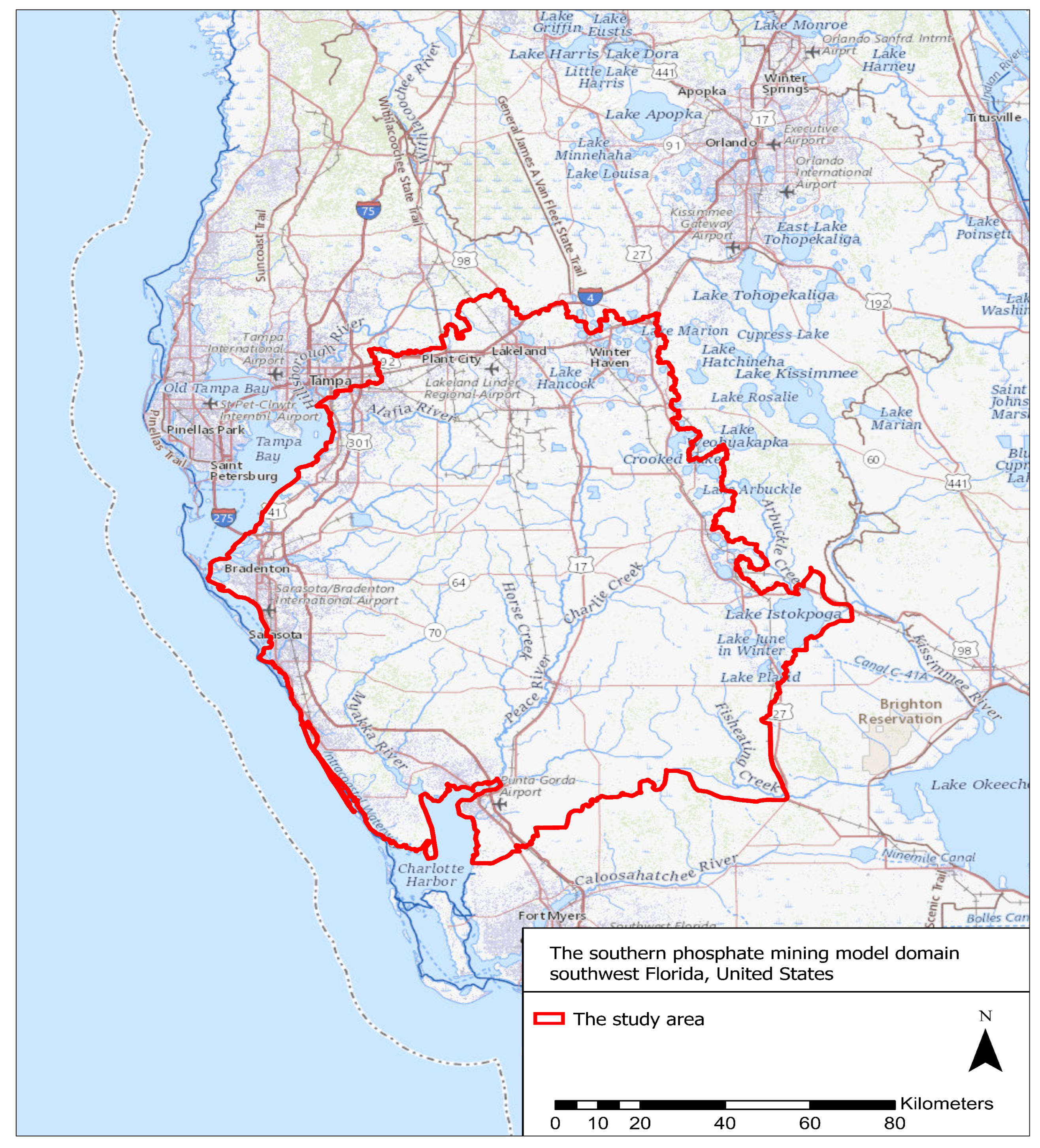
Study Area
2. Methodology
2.1. Rivers and Streams’ RCHRES
2.1.1. Discharge Rating Curve Characterization for Rivers and Streams’ RCHRES
2.1.2. Characterization of Pool Storage for Streams and Rivers’ RCHRESs
2.2. Wetlands and Lakes’ RCHRESs
Discharge Rating Curves for Wetlands’ RCHRES
2.3. Discharge Rating Curves for Lakes’ RCHRES
2.3.1. Storage Rating Curves for Wetlands and Lakes’ RCHRESs
2.3.2. Stage–Storage within Soils
2.3.3. The Semi-Automated Spreadsheets Generator for F-Tables
2.3.4. Model Validation and Water Budget Analysis
2.4. Results and Discussion
2.4.1. Nilsson’s [31] Shape Parameter for Alluvial Systems, and
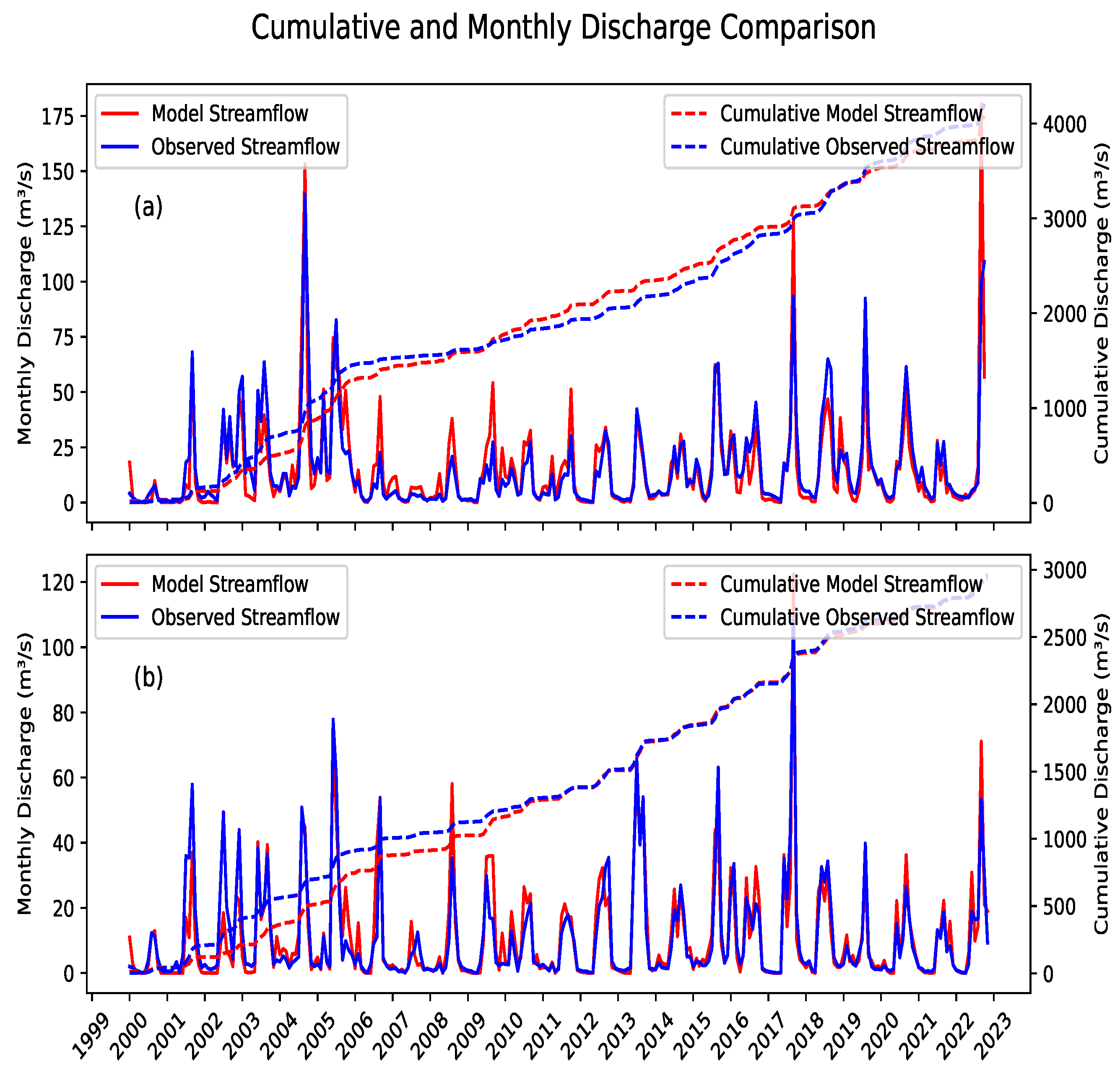
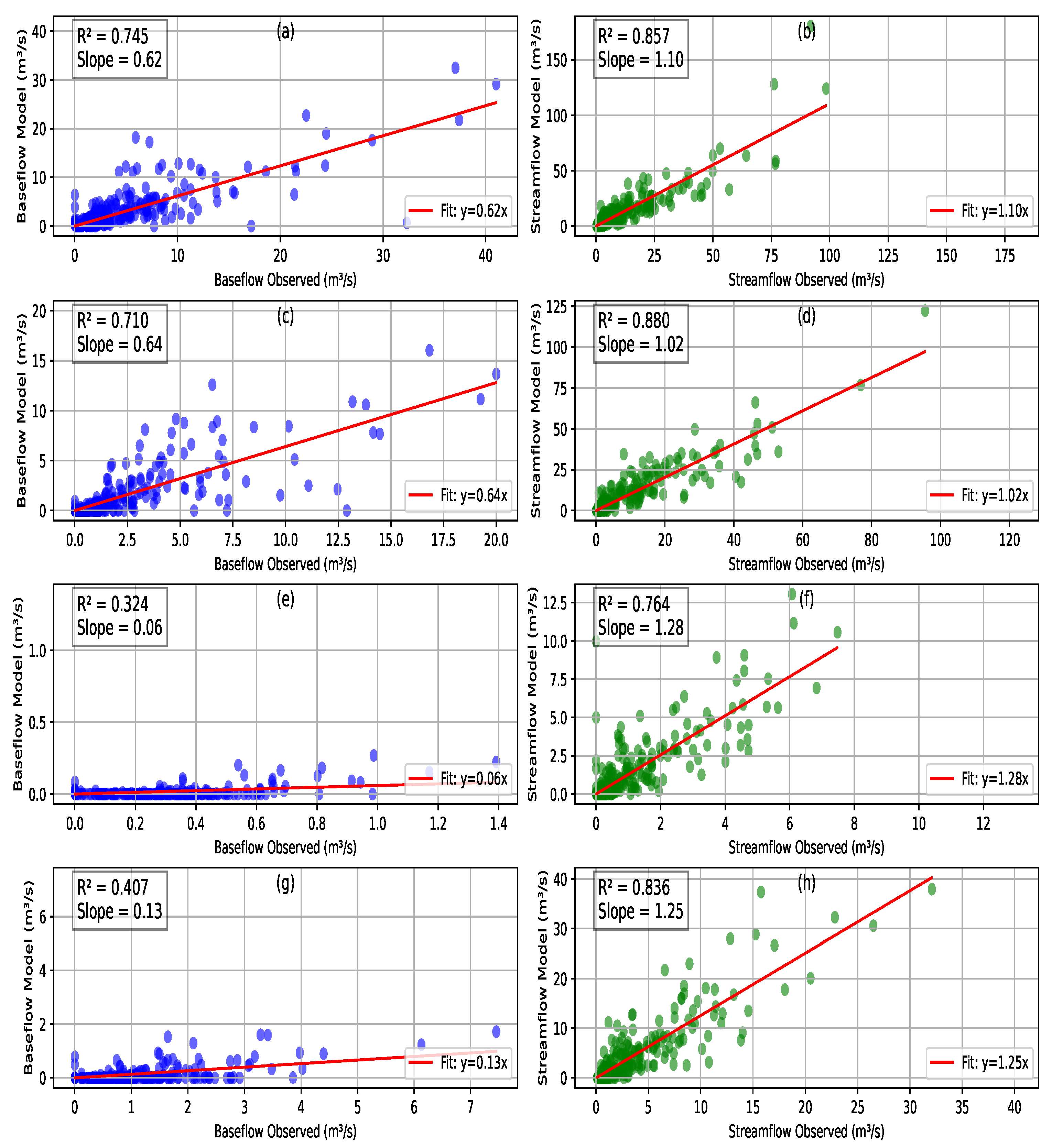
2.4.2. Model Validation
2.5. Conclusions
Author Contributions
Funding
Data Availability Statement
Acknowledgments
Conflicts of Interest
References
- Chelsea Nagy, R.; Graeme Lockaby, B.; Kalin, L.; Anderson, C. Effects of urbanization on stream hydrology and water quality: The Florida Gulf Coast. Hydrol. Process. 2012, 26, 2019–2030. [Google Scholar] [CrossRef]
- Lewelling, B.R.; Wylie, R.W. Hydrology and water quality of unmined and reclaimed basins in phosphate-mining areas, west-central Florida. US Geol. Surv. 1993, 93, 4002. [Google Scholar]
- Florea, L.J. Geology and Hydrology of Karst in West-Central and North-Central Florida. Ph.D. Thesis, University of South Florida, Tampa, FL, USA, 2008. [Google Scholar]
- Dahl, T.E. Wetlands Losses in the United States, 1780’s to 1980’s; US Department of the Interior, Fish and Wildlife Service: Falls Church, VA, USA, 1990.
- Haag, K.H.; Lee, T.M. Hydrology and Ecology of Freshwater Wetlands in Central Florida—A Primer. U.S. Geological Survey Circular 1342, U.S. Geological Survey. 2010. Available online: https://pubs.usgs.gov/circ/1342/ (accessed on 13 January 2024).
- Viessman, W. Water Management: Challenge and Opportunity. J. Water Resour. Plan. Manag. 1990, 116, 155–169. [Google Scholar] [CrossRef]
- Zhang, J.; Ross, M.; Trout, K.; Zhou, D. Calibration of the HSPF model with a new coupled FTABLE generation method. Prog. Nat. Sci. 2009, 19, 1747–1755. [Google Scholar] [CrossRef]
- Gupta, R.S. Hydrology and Hydraulic Systems; Waveland Press: Long Grove, IL, USA, 2016. [Google Scholar]
- Bowers, R.T. Quantifying a 21-Year Surface Water and Groundwater Interaction in a Ridge and Valley Lake Environment Using a Highly Constrained Modeling Approach. Ph.D. Thesis, University of South Florida, Tampa, FL, USA, 2022. [Google Scholar]
- Hwang, S.; Graham, W.D.; Geurink, J.S.; Adams, A. Hydrologic implications of errors in bias-corrected regional reanalysis data for west central Florida. J. Hydrol. 2014, 510, 513–529. [Google Scholar] [CrossRef]
- Zhang, J.; Ross, M. Hydrologic simulation of clay-settling areas in the phosphate mining district, Florida: Hydrologic simulation of csas in the phosphate mining district. Hydrol. Process. 2012, 26, 3770–3778. [Google Scholar] [CrossRef]
- Ross, M.; Geurink, J.; Said, A.; Aly, A.; Tara, P. EVAPOTRANSPIRATION CONCEPTUALIZATION IN THE HSPF-MODFLOW INTEGRATED MODELS. J. Am. Water Resour. Assoc. 2005, 41, 1013–1025. [Google Scholar] [CrossRef]
- Bicknell, B.R.; Imhoff, J.C.; Kittle, J.L.; Donigian, A.S. Hydrological Simulation Program—Fortran User’s Manual for Release 1; US Environmental Protection Agency: Athens, Greece, 1997.
- Miller, J.A. Hydrogeologic Framework of the Floridan Aquifer System in Florida and in Parts of Georgia, Alabama, and South Carolina; Professional Paper 1403-B; United States Geological Survey: Reston, VA, USA, 1986.
- Vacher, H.L.; Mylroie, J.E. Eogenetic karst from the perspective of an equivalent porous medium. Carbonates Evaporites 2002, 17, 182–196. [Google Scholar] [CrossRef]
- Budd, D.A.; Vacher, H.L. Matrix permeability of the confined Floridan Aquifer, Florida, USA. Hydrogeol. J. 2004, 12, 531–549. [Google Scholar] [CrossRef]
- Luesaksiriwattana, N. The Impact of Land Use Change on Hydrology Using Hydrologic Modelling and Geographical Information System (GIS). Master’s Thesis, University of South Florida, Tampa, FL, USA, 2022. [Google Scholar]
- Yeh, P.J.; Famiglietti, J.S. Regional groundwater evapotranspiration in Illinois. J. Hydrometeorol. 2009, 10, 464–478. [Google Scholar] [CrossRef]
- Chintalapudi, S.; Sharif, H.O.; Yeggina, S.; Elhassan, A. Physically Based, Hydrologic Model Results Based on Three Precipitation Products 1. JAWRA J. Am. Water Resour. Assoc. 2012, 48, 1191–1203. [Google Scholar] [CrossRef]
- Skinner, C.; Bloetscher, F.; Pathak, C.S. Comparison of NEXRAD and Rain Gauge Precipitation Measurements in South Florida. J. Hydrol. Eng. 2009, 14, 248–260. [Google Scholar] [CrossRef]
- Wang, Y.Q.; Xiong, Y.J.; Qiu, G.Y.; Zhang, Q.T. Is scale really a challenge in evapotranspiration estimation? A multi-scale study in the Heihe oasis using thermal remote sensing and the three-temperature model. Agric. For. Meteorol. 2016, 230, 128–141. [Google Scholar] [CrossRef]
- Cai, J.; Liu, Y.; Lei, T.; Pereira, L.S. Estimating reference evapotranspiration with the FAO Penman–Monteith equation using daily weather forecast messages. Agric. For. Meteorol. 2007, 145, 22–35. [Google Scholar] [CrossRef]
- Liu, C.; Zhang, D.; Liu, X.; Zhao, C. Spatial and temporal change in the potential evapotranspiration sensitivity to meteorological factors in China (1960–2007). J. Geogr. Sci. 2012, 22, 3–14. [Google Scholar] [CrossRef]
- Liu, Y.J.; Chen, J.; Pan, T. Analysis of Changes in Reference Evapotranspiration, Pan Evaporation, and Actual Evapotranspiration and Their Influencing Factors in the North China Plain during 1998–2005. Earth Space Sci. 2019, 6, 1366–1377. [Google Scholar] [CrossRef]
- Zhang, L.; Dawes, W.R.; Walker, G.R. Response of mean annual evapotranspiration to vegetation changes at catchment scale. Water Resour. Res. 2001, 37, 701–708. [Google Scholar] [CrossRef]
- Geurink, J.S.; Basso, R. Development, Calibration, and Evaluation of the Integrated Northern Tampa Bay Hydrologic Model. Prepared for Tampa Bay Water, Clearwater, FL and the Southwest Florida Water Management District, Brooksville, FL. 2013. Available online: https://integratedhydrologicmodel.org/publications (accessed on 13 January 2024).
- Alshehri, F.; Ross, M. Advancing Discharge Ratings: A Novel Approach Based on Observed and Derivable GIS Factors in Alluvial Systems. Water 2023, 15, 4152. [Google Scholar] [CrossRef]
- Alshehri, F.; Ross, M. Calibrating Complexity: A Comprehensive Approach to Developing Stage–Storage–Discharge Relationships for Geographically Isolated Wetlands (GIWs) in W-C Florida. Water 2023, 15, 3878. [Google Scholar] [CrossRef]
- Doherty, J. PEST-ASP User’s Manual; Watermark Numerical Computing: Brisbane, Australia, 2001. [Google Scholar]
- Mueses-Pérez, A. Generalized Non-Dimensional Depth-Discharge Rating Curves Tested on Florida Streamflow. Ph.D. Thesis, University of South Florida, Tampa, FL, USA, 2006. Available online: https://digitalcommons.usf.edu/etd/2639 (accessed on 13 January 2024).
- Kenneth Allan, N. Improved Methodologies for Modeling Storage and Water Level Behavior in Wetlands. Ph.D. Thesis, University of South Florida, Tampa, FL, USA, 2010. Available online: https://digitalcommons.usf.edu/etd/1723 (accessed on 13 January 2024).
- Streamline-Technologies. ICPR4 Technical Reference Manual; Streamline-Technologies: Winter Springs, FL, USA, 2018. [Google Scholar]
- Lee, T.M. Factors Affecting Ground-Water Exchange and Catchment Size for Florida Lakes in Mantled Karst Terrain; Report Number, 2; US Department of the Interior: Washington, DC, USA; US Geological Survey: Reston, VA, USA, 2002.
- Shah, N. Vadose Zone Processes Affecting Water Table Fluctuations: Conceptualization and Modeling Considerations. Ph.D. Thesis, University of South Florida, Tampa, FL, USA, 2007. Available online: https://digitalcommons.usf.edu/etd/2360. (accessed on 13 January 2024).
- Perry, R.G. Regional Assessment of Land Use Nitrogen Loading of Unconfined Aquifers. Ph.D. Thesis, University of South Florida, Tampa, FL, USA, 1995. [Google Scholar]


| Parameter | Description |
|---|---|
| Hydrology type | Coastal plain hydrology |
| Geographical area | 14,090 km2 |
| Soil type | Sandy soil |
| Climate zone | Humid subtropical |
| Wet season duration | June to October (about 2/3 of annual rainfall) |
| Dry season duration | November to May (about 1/3 of annual rainfall) |
| Average annual rainfall | ≈1320 mm (52 inches) |
| Potential evapotranspiration | ≈1320 mm (52 inches) |
| Groundwater environment | Shallow groundwater environment |
| Total hydrography area | 383,248 km2 |
| Number of wetlands | 148,000 wetlands |
| Number of USGS streamflow gauging stations | 28 |
| Number of NEXRAD GAR stations | 66 |
| Number of reference evapotranspiration stations | 13 |
| Natural Landscape Features | Hydrological Response Unit (HRU) | Percentage |
|---|---|---|
| Uplands | Urban Impervious | 2.7% |
| Urban pervious | 13.1% | |
| Low-slope grassland | 25.8% | |
| High-slope grassland | 5.5% | |
| Flatwoods | 5.1% | |
| Hardwoods | 4.0% | |
| Mining | 3.1% | |
| Irrigated row crop | 4.1% | |
| Irrigated tree crop | 9.5% | |
| Total uplands | 72.8% | |
| Hydrofeatures | Wetlands | 6.9% |
| Streams | 16.7% | |
| Rivers | 2.4% | |
| Lakes | 1.2% | |
| Total hydrofeatures | 27.2% |
| Equations | Description |
|---|---|
| is the 50th-percentile daily exceedance (m3/s), is the drainage area (km2), , | |
| is the 10th-percentile daily exceedance (m3/s), , | |
| is the 1st-percentile daily exceedance (m3/s), , | |
| is the cross-section area of (m2), is the channel slope (m/m), , , | |
| is the hydraulic depth of (m), is the channel width (m) | |
| is the depth of (m), , | |
| is the depth of (m), , | |
| is the depth of (m), , |
Disclaimer/Publisher’s Note: The statements, opinions and data contained in all publications are solely those of the individual author(s) and contributor(s) and not of MDPI and/or the editor(s). MDPI and/or the editor(s) disclaim responsibility for any injury to people or property resulting from any ideas, methods, instructions or products referred to in the content. |
© 2024 by the authors. Licensee MDPI, Basel, Switzerland. This article is an open access article distributed under the terms and conditions of the Creative Commons Attribution (CC BY) license (https://creativecommons.org/licenses/by/4.0/).
Share and Cite
Alshehri, F.; Ross, M. Application and Evaluation of Stage–Storage–Discharge Methodology in Hydrological Study of the Southern Phosphate Mining Model Domain in Southwest Florida. Water 2024, 16, 842. https://doi.org/10.3390/w16060842
Alshehri F, Ross M. Application and Evaluation of Stage–Storage–Discharge Methodology in Hydrological Study of the Southern Phosphate Mining Model Domain in Southwest Florida. Water. 2024; 16(6):842. https://doi.org/10.3390/w16060842
Chicago/Turabian StyleAlshehri, Fahad, and Mark Ross. 2024. "Application and Evaluation of Stage–Storage–Discharge Methodology in Hydrological Study of the Southern Phosphate Mining Model Domain in Southwest Florida" Water 16, no. 6: 842. https://doi.org/10.3390/w16060842
APA StyleAlshehri, F., & Ross, M. (2024). Application and Evaluation of Stage–Storage–Discharge Methodology in Hydrological Study of the Southern Phosphate Mining Model Domain in Southwest Florida. Water, 16(6), 842. https://doi.org/10.3390/w16060842