Article

A Framework for Assessment of Flood Conditions Using Hydrological and Hydrodynamic Modeling Approach

1
Department of Civil Engineering, Indian Institute of Technology Delhi, Hauz Khas, New Delhi 110016, India
2
Haskoning DHV Consulting Pvt Ltd., Green Boulevard, Sector 62, Noida 201301, India
*
Author to whom correspondence should be addressed.
Water 2023, 15(7), 1371; https://doi.org/10.3390/w15071371
Submission received: 12 February 2023 / Revised: 12 March 2023 / Accepted: 21 March 2023 / Published: 3 April 2023

Abstract

:
River flooding has been triggering significant damage to lives and infrastructure and is a major worry all around the globe. To lessen these losses, proper planning and management methods need to be deployed. The purpose of this research is to fill a knowledge gap on the effects of reservoirs operation of the Idukki and Idamalyar to Periyar River Basin massive flooding. The proposed methodology is implemented on the Periyar River Basin located in Kerala, India, where severe flooding occurred during monsoon season in the year 2018. In this study, modelling technique has been used in two-step: (1) development of 1D physically based, distributed-parameter model (Soil and Water Assessment Tool, SWAT) to compute the stream flow and estimate the stream discharge at different outlet points; and (2) hybrid model is developed by linking SWAT with a well-known 2D hydrodynamic model (International River Interface Cooperative, iRIC) to display flood scenarios and to identify the flood-prone areas. The ArcSWAT user interface employed in the ArcGIS software was utilized to delineate the river basin. The SWAT model was calibrated and validated on daily and monthly basis at two gauge discharge stations, i.e., Neeleeswaram and Kalady. The statistical coefficients result obtained from SWAT model was in good agreement with the measured values for calibration and validation. The hybrid model simulation results compared with observed flood depth and remote sensing data demonstrated good capability of the model. Agreeable performances of computed results were observed in both flow fields and flood propagations. The result was compared with 2018 flood to check model accuracy and found to be satisfactory. The proposed framework can be utilized as an effective tool for efficient planning and management of natural disasters, such as flash floods.

1. Introduction

Worldwide, catastrophic floods have caused massive destruction to society. Several disaster information reports and databases indicate that flooding has been increasing globally and causing massive financial losses, particularly in the past decades [1,2,3] (Due to the limitations of recorded flooding data and the complexity in splitting the confounding land use and water management impacts of floods, various studies have emphasized the significance of investigating the role of anthropogenic interventions in reducing severe flooding [4,5,6], and noting that an integrated method for flood analysis is needed. One of the most disastrous floods that hit Kerala in 2018 happened in the Periyar River basin. Heavy rainfall caused flood peaks that exceeded the projected return period of 100 years peak discharge.
Extreme weather events and associated floods that cause serious destruction to people, property, and the ecosystem are topics of worldwide concern. India has experienced extreme floods over the past two decades due to intense rainfall, including Maharashtra 2005 flood in Mumbai, Bihar 2008 in Kosi, Andhra Pradesh 2009 in Krishna, Jammu and Kashmir 2010 in Leh, and Ladakh, Uttarakhand 2013 in Kedarnath and Tamil Nadu 2015 in Chennai [7]. The scale of livestock and human deaths, crop damage, and financial loss from floods was immense [8]. The estimated damage cost from flood damage in India between 1953 and 2016 is estimated to be approximately 347,581.201 crore rupees [9]. In August 2018, Kerala (India) faced some of the heaviest extreme precipitation events on record. As a result, large-scale floods and landslides have occurred in most counties of the state, causing serious harm to both constructed and natural ecosystems.
Between 1 June 2018 to 19 August 2018, 2346.6 mm rainfall was received by Kerala state during summer, which is much higher (about 42%) than usual precipitation during the same duration. Idukki district received the maximum precipitation, i.e., 3555 mm compared to the normal 1852 mm (almost 100% more) amongst all the districts of Kerala state. Around 164.4% excess rainfall occurred in Kerala during two events, i.e., between the days of 8–10 and 14–19 in the month of August. Kerala’s high-altitude physical geography supports many dams and reservoirs and is designed primarily for hydropower and irrigation purposes. The monsoon started during the start of the June 2018 and all the reservoirs filled up to full reservoir level (FRL) by July 2018. This unusual blend of precipitation and filled reservoir (FRL) made the condition very problematic, pushing the agencies to wide open the dams’ gates in almost all the districts except one (13 out of 14) thus, causing serious flooding in the state. In recent years, several studies have been carried out by researchers to compute flood inundation using hydrodynamic modeling techniques to simulate floodplains [10,11].
There are numbers of numerical models available in the literature for delineating floodplain inundation and for simulating flow. The developed model can help in mapping river floodplain zones and estimate the risk associated with it for different return periods. These mathematical models are divided into three types: 1D (one-dimensional) models, 2D (two-dimensional) models, and hybrid model, i.e., coupling of 1D River flow models with 2D floodplain flow models. Though 1D models are easy to utilize and deliver data on bulk flow attributes, they do not give field flow information. Additionally, 2D models involve longer computational time, so an effort has been made to develop hybrid model by coupling SWAT (1D river flow models) with iRIC (2D floodplain flow models). Such types of models is exceptionally efficient for real-time flood events computation [12,13].
In Periyar River basin two hydro-electric projects are situated at Idukki and Idamalayar districts which control flood apart from generating power. The present study examines the effect of flooding in the reservoirs of Idukki and Idamalayar in relation to the storage regime (inflow and outflow). A significant amount of flood water is accumulated in these two reservoirs. The significance of non-meteorological components, such as reservoir control, in determining the magnitude of the disaster. Previous studies have reported that the Idukki and Idamalayar reservoirs in the basin are major reservoirs having significant impact on the River Basin’s hydrologic regime. The majority of researchers have concentrated on reservoir operation optimization in comparatively smaller watershed. None of the previous studies have employed coupled 1D and 2D model for investigating and reviewing the effects of reservoir operation on the complete river basin. The purpose of this research is to fill a knowledge gap on the effects of reservoirs operation of the Idukki and Idamalyar to Periyar River Basin massive flooding.
To address this issue, two main objectives for the present study is formulated: (1) development of SWAT and iRIC based coupled hydrological and hydrodynamic model for simulating operation of reservoir and its effects to flooding extent in the river watershed, and (2) to establish the advantages of the developed model in evaluating alternate operation rules for reservoirs, which can possibly lessen flooding. To the best of the authors’ knowledge, a similar type of work has never been carried out for Idamalyar and Idukki reservoirs. To address the gap more precisely, the subsequent subobjectives have been carried out: (a) combined hydrologic and hydrodynamic model has been developed, (b) preparation of algorithms for operating Idukki and Idamalyar reservoirs to suggest alternate reservoirs operation rules, (c) validation of the combined model’s capability in simulating regulated flows and flood inundation, and (d) comprehensive investigation of the effects of alternate reservoir operation rules for flood inundation in the Periyar River watershed. This is for the first time, as per the knowledge of the authors, that coupled SWAT Hydrological model and 2D iRIC simulations were applied to address flood effects in the downstream area of the coastal region due to Idukki and Idamalyar dam taking tidal effect as boundary conditions. For the 2D model development upstream river flow and downstream tidal effects were considered. The model output parameters flow rate, flood inundation time, depth, and velocity, and flood inundation extent at different scenarios have been ascertained.

2. Study Area

Periyar River Basin is situated on the south most portion of the western coastline in the Kerala state, India. The Kerala state observed the Indian Summer Monsoon Rainfall (ISMR), which normally begins from the coastal region, and receives the maximum monsoon precipitation. The yearly average precipitation received by the state is about 3000 mm along with substantial spatial inconsistency within the state. Around 50% of the yearly rainfall is received during the months of June and July. The topography of Kerala indicates a broad variety varying from rocky zig-zag uplands to soft plains in coastal area. The state width (i.e., the distance between the coastal line and Western Ghat’s ridgeline) differs from 15 km to 120 km. The soft plain in coastal region is heavily inhabited, and the rest highland and midland regions are primarily used for different plantations and agricultural activities. The coastal line and Western Ghat’s ridgeline have very limited width in conjunction with heavy populace make the basins prone to flooding because it has lesser response time to intense rainfall occurrences. Figure 1 shows the longest river in the state of Kerala, i.e., Periyar River having total length of 244 km. Tributaries, such as Muthirapuzha, Mullayar, Idamalayar, Perinjankutty Ar, and Cheruthoni Ar are the major tributary flowing through steep valleys and deep gorges.
Normally the state has a dendritic type of drainage pattern in nature. The Periyar River splits into two streams at Alwaye, which outfalls into the Arabian Sea via two separate estuaries. The river is severely controlled by Idukki and Idamalayar reservoirs, built primarily for irrigation and power generation. The reservoirs’ geographical position is marked in Figure 1. The major reservoir of the basin is Idukki reservoir managed by three dams, i.e., Idukki dam, Kulamavu dam, and Cheruthoni dam. Amongst the different dams, the major dams are the Idamalayar and Idukki–Cheruthoni–Kulamavu trio. The Idamalayar and Periyar Valley Irrigation Project are the major irrigation projects in the basin.

3. Hydrological and Hydrodynamic Models

3.1. SWAT Model

Soil and Water Assessment Tool (SWAT) is a physical based semi-empirical model that can model any size watershed area. SWAT estimates flow and transportation of sediment by utilizing numerous parameters which affect the hydrological cycle. The SWAT is created to estimate the performance of land controlling on water, agricultural, and sediment in dense, huge watersheds for longer periods wherever the situations, such as land use, soil type, and its management varies [14]. Additionally, the model proposes non-preventable modelling with excellent spatial information by splitting the watershed into different sub-watersheds. Hydrologic response units (HRUs) are acquired by further splitting the sub-watersheds, which carry different soil features, land use, and its managing procedures. The model was created by the Blackland Research Centre. Initially the SWAT model was built in C language, and afterwards, had made to fit with GRASS [15]. Bian et al. [16] established a new version in Arc Macro Language, which was user-friendly with ArcInfo, and later, in Avenue to make it pleasant with ArcView [17].
Computation is split up into two distinct stages to examine the hydrology of catchment. They are the land and routing stage of the hydrological cycle. In the land stage, it regulates volume of water and sediment loads into the watercourse for specific sub-watershed. Evapotranspiration, infiltration, storage, redistribution, lateral subsurface flow, overland flow, sections of channels return flow, and ponds are the elements calculated in land stage of the hydrological cycle. However, in the routing stage runoff movement and sediments that flow across the river into the outlet from the catchment are considered. In the land stage, SWAT employed equation of water balance to estimate the hydrological cycle (Equation (1)).
S W t = S W 0 + i = 1 t [ P i Q s u r f E a W s e e p Q g w ]
where SWt is soil water final content in mm, SWo is soil water initial content on ith day in mm, t is time (days), Pi is rainfall amount on ith day in mm, Qsurf is surface runoff amount on ith day in mm, Ea is evaporation amount on ith day in mm, Wseep is quantity of water go into the vadose zone from the soil profile on ith day in mm, and Qgw is quantity of groundwater flow on ith day in mm.
Important parameters of the model is described below. For a comprehensive description on SWAT parameters, please refer Arnold et al., [18], and Neitsch et al., [19]. Surface runoff is generated when infiltration is less than the rainfall. The two techniques, i.e., Green Ampt infiltration method [20] and SCS curve number procedure [21], are employed to calculate runoff. For each HRUs, peak runoff and quantity of overland flow is calculated by utilizing sub-daily and daily rainfall in SWAT. In Equation (2), SCS curve number technique is used to evaluate the watershed’s runoff:
Q s u r f = ( R d a y 0.2 S ) 2 ( R d a y + 0.8 S )
where Qsurf is rainfall in excess in mm, Rday is depth of rainfall for the day in mm, and S is the retention parameter in m).
Equation (3) explains the retention parameter:
S = 25.4 [ 1000 C N 10 ]
where CN is curve number for the day.
There are two techniques in SWAT to determine retention parameters. In the first technique, by altering the content of water content in the soil profile, the retention parameters are computed, whereas in second technique, by varying the plant evapotranspiration, retention parameters is estimated. In shallow soils, the runoff is overestimated when soil moisture technique (Equation (4)) is employed. Whereas CN is determined for plant evapotranspiration on daily basis, where CN value is more dependent on antecedent climate than soil storage.
S = S m a x [ 1 S W [ S W + e x p ( w 1 w 2 S W ) ] ]
where S is retention parameter for a given day in mm, Smax is maximum value that the retention parameter can have on any given day in mm, SW is soil water content of the entire profile excluding the quantity of water held in the profile at wilting point in mm, and w1 and w2 are coefficients of shape.
The maximum retention parameter value, Smax, is determined by computing Equation (5) utilizing CN1:
S m a x = 25.4 [ 1000 C N 1 10 ]
Retention parameters differ due to plant evapotranspiration. In such environments, to make the retention parameter updated daily, subsequent equations are utilized:
S = S p r e v + E a e x p [ c n c o e f S p r e v S m a x ] R d a y Q s u r f
where Sprev is retention parameter for the previous day in mm, Ea is potential evapotranspiration for the day in mm/day, cncoef is weighting coefficient utilized to compute the retention coefficient for daily curve number estimates, Smax is maximum value retention parameter that can achieve on any given day in mm, Rday is rainfall depth for the day in mm, and Qsurf is surface runoff in mm. The retention parameter initial value is defined as: S = 0.9 S m a x .
The functions of SCS curve numbers are Land use, antecedent soil water conditions and permeability of soil. The three antecedent moisture environments are defined by SCS, i.e., I—dry (wilting point), II—average moisture, and III—wet (field capacity). To calculate the curve numbers for moisture conditions I and III, Equations (7) and (8) are utilized
C N 1 = C N 2 [ 20 × ( 100 C N 2 ) 100 C N 2 + e x p [ 2.533 0.063 ( 100 C N 2 ) ] ]
C N 3 = C N 2 × e x p [ 0.00673 × ( 100 C N 2 ) ]
Neitsch [19] offered the standard CN values for moisture conditions II, which are appropriate for five percent slope gradient. At different slopes, Equation (9) is utilized to tune the CN value [22].
C N 2 ( s ) = ( C N 3 C N 2 3 ) × [ 1 2 × exp ( 13.86 × s l p ) ] + C N 2
where CN1 is antecedent moisture condition I curve number, CN2 is antecedent moisture condition II curve number, CN3 is antecedent moisture condition III curve number for the default 5% slope, CN2(S) is moisture condition II curve number adjusted for slope, and slp is average percent slope of sub basin.
In the SWAT model, enhanced form of rational technique can be employed to estimate the peak surface runoff as presented in Equation (10).
q p e a k = α t c × Q s u r f × A r e a 3.6 × t c o n c
where qpeak is peak runoff rate in m3/s, αtc is fraction of daily rainfall that occurs during the time of concentration, Qsurf is surface runoff in mm, and tconc is time of concentration for the sub-basin (h), with conversion factor of 3.6.
For evaluating potential evapotranspiration (PET), there are three methods, i.e., Penman-Monteith method [23], Hargreaves method [24], and Priestley-Taylor method [25] are unified in SWAT. For modelling groundwater, a deep confined aquifer and unconfined aquifer (shallow) are the two aquifers represented in the SWAT. Amongst the two, the aquifer which improves the flow to the stream network or to the sub-watersheds is the unconfined aquifer [26].
SWAT model’s strength is that it is an effective computer-based model that can compute any watershed, even if generic data, such as stream gauge data, is unavailable. For modelling larger watershed, the computation time is minimal and cheap. Having said that limitations of the model also exist, as reported by some researcher [27]. The model simulates on a continuous daily time step, but it cannot perform satisfactory for event-based simulation [28]. Similarly, the curve-number module utilized to calculate run-off proposes assumptions for soil factors which are not same for all watersheds.

3.2. iRIC Model

The International River Interface Cooperative (iRIC) model product offers a unified river model environment. iRIC offers a complete, integrated environment in which compilation of necessary data required for river analysis solvers can be completed so that computation of the rivers can be performed, and results can be visualized.
NAYS2DFLOOD: Nays2DFlood is a flood flow solver after editing the Nays2D code designed by Shimizu [29]. The model is neither available for sediment transport nor for bed evolution, but it includes similar theories and coordinate system. Later, changes to the model, involving the adding of pumps, culverts, weirs, etc., to deliver practical depiction of flood discharge were made. The solver also allows the modeler to set any random inflow that is entering rivers. It is freely available open-source software. The interface of the model explains runoff and morphological performance in the river. For more detailed about its invention and solvers, is available in iRIC software package [30].
The model provides a comprehensive unified structure where the common generalized info needed by the solvers can be gathered, the simulation can be completed, and result can be evaluated. Figure 2 explains the typical procedures of the model. The continuity and the momentum equations, for 2D unsteady flow is given [31]:
Equation of Continuity:
h t + ( h u ) x + ( h v ) y = 0
Equation of Momentum:
( h u ) t + ( h u 2 ) x + ( h u v ) y = g h H x τ b x ρ + x ( V ( h u ) x ) + y ( V ( h u ) y )
( h u ) t + ( h u v ) x + ( h v 2 ) y = g h H y τ b y ρ + x ( V ( h v ) x ) + y ( V ( h v ) y )
where h = depth of water; u, v = components of depth averaged velocity, τb= shear stress of bed, ρ = density of water, H = stage height (H = h + zb), zb = elevation of bed, ν = eddy viscosity t = time, and x, y = spatial coordinate components in the Cartesian system. The bed shear stress components is given below as:
τ b x = ρ C f u ( u 2 + v 2 )  
τ b y = ρ C f v ( u 2 + v 2 )
v = k 6
where Cf = coefficient of bed friction, k = Karman constant, and u = shear velocity.
The above equations are in the Cartesian coordinate system. The Jacobian chain rules were employed to transform them into moving boundary fitted coordinate system.
The Cubic Interpolation Pseudoparticle (CIP) method, also called the high-order Gudunov scheme, was utilized for the application of water flow equations. The variables are spatially interpolated at the prior time step by utilizing the cubic interpolation along with some assumption. The spatial gradients were also transported by employing alike convective equations. Information on a small number of adjacent cells is sufficient for this method to calculate exact profiles of convectional variables. The variations in the flow and floodplain configuration are mathematically calculated at very small-time step allowed by its CFL standard.

4. Model Efficiency

Numerous statistical techniques are available in the literature to read check results accuracy generated by the model. The calibration and the validation were conducted utilizing two usually utilized statistic coefficients parameter [32,33]. These statistical techniques are Nash Sutcliffe Efficiency index (NSE) and Percent Bias (PBIAS).

4.1. Nash Sutcliffe Efficiency Index

NSE is a standard statistical technique employed for estimating the noises. It is represented by Nash and Sutcliffe [34] and is computed from the equation given below (Equation (17)):
NSE = 1 i = 1 n ( Y i o b s Y i s i m ) 2   i = 1 n ( Y i o b s Y m e a n ) 2
where Yobsi is the ith monitoring of stream flow, Ysimi is the ith computed value, Ymean is average of monitored data, and n is number of total monitored data. NSE vary between 0.0 and 1.0 are normally considered as satisfactory levels of operation. Usually, for satisfactory model results, NSE should be greater than 0.5, whereas 1 signifies optimal value [32].

4.2. Percent Bias

PBIAS calculates the average trend of computation to be greater or less than corresponding monitored data [35]. Equation (18) is employed to calculate PBIAS and is given below:
PBIAS = i = 1 n ( Y i o b s Y i s i m ) 100 i = 1 n ( Y i o b s )
PBIAS = 0.0 implies optimal value. Furthermore, positive and negative values of PBIAS implies that the model is under-predicting and over-predicting, respectively, and is recommended by ASCE for use.

5. Results and Discussion

5.1. Hydrological Modelling—SWAT

5.1.1. Model Development

The ArcSWAT 2012 interface uses SWAT 2012 version, which is a basin level, continuous time step hydrology model that can deliver model outcome on annual basis, monthly basis and daily basis [36]. ArcSWAT delineates watershed and divides it into sub-catchment by utilizing Digital Elevation Map (DEM), land use, soil type, and weather data. Sub-watershed parameters, such as the slope gradient and slope length of the terrain, were derived from the DEM. For the study data of land use (LU/LC) of 2010 procured from National Remote Sensing Centre, Indian Space Research Organization (ISRO). The land use mainly dominated by agricultural and forest land. Soil type and DEM were obtained from National Bureau of Soil Survey and Landuse Planning (NBSS-LUP), and Shuttle Radar Topography Mission (SRTM), USGS. The required weather data, such as precipitation, temperature (minimum and maximum), were acquired from Indian Meteorological Department (IMD)—Pune, India at daily time step. The river reach, location of reservoirs and gauging station land use, soil, and slope are shown in Figure 3.

5.1.2. Calibration and Validation of the Model

In the SWAT model, the discharge estimation depends on 12 parameters. To identify the most sensitivity parameters responsible for discharge calculation in Periyar river basin, sensitivity analysis was carried out in ArcSWAT, taking all 12 parameters into consideration. After the analysis, it was found that only five were observed to be more sensitive and only these parameters were studied for calibration procedure. Sensitivity analysis was performed to decide the impact of twelve discharge parameters set to undergo sensitivity in ArcSWAT. These parameters are (1) SCS runoff curve number for moisture condition II (r_CN2.mgt), (2) Base Flow Alpha factor (v_ALPHA_BF.gw), (3) Threshold depth of water in the shallow aquifer required for return flow to occur in mm (v_GWQMN.gw), (4) Ground Water ‘Revap’ Coefficient (v_GW_REVAP.gw), and (5) Manning’s ‘n’ value for main Channel (r_CH_N2.rte) is given in details in Table 1.
Other parameters are: (1) Soil Evaporation Compensation Factor (ESCO), (2) Ground Water Delay Time (GW DELAY.gw), (3) Available Water Capacity (SOL AWC.sol), (4) Plant uptake compensation factor (EPCO.bsn), (5) Hydraulic conductivity of reservoir bottom (RES_K.res), (6) Surface runoff lag time (SURLAG.bsn), and (7) Initial depth of water in the shallow aquifer (SHALLST.gw).
The calibration of the SWAT model was performed on a daily and monthly time scale between 1 January 1996 to 31 December 2001, and for validation between 1 January 2002 and 31 December 2015 at Neeleeshwaram station, and at Kalady station, the calibration period were between 1 January 2002 to 31 December 2010, and validation between from 1 January 2011 and 31 December 2017. In both cases, 5 years before the calibration is considered as the warming period. The output computed from the calibration procedure is shown in Figure 4. A comparison between computed and monitored stream discharge at both the station on daily and monthly basis was also performed (Figure 4), which shows satisfactory result (Table 1). The model captured well on daily and monthly time series of stream flow, as can be seen from the NSE and PBIAS value (Table 2). The model is following the flow trend and almost predicting the flow on monthly and on daily basis.

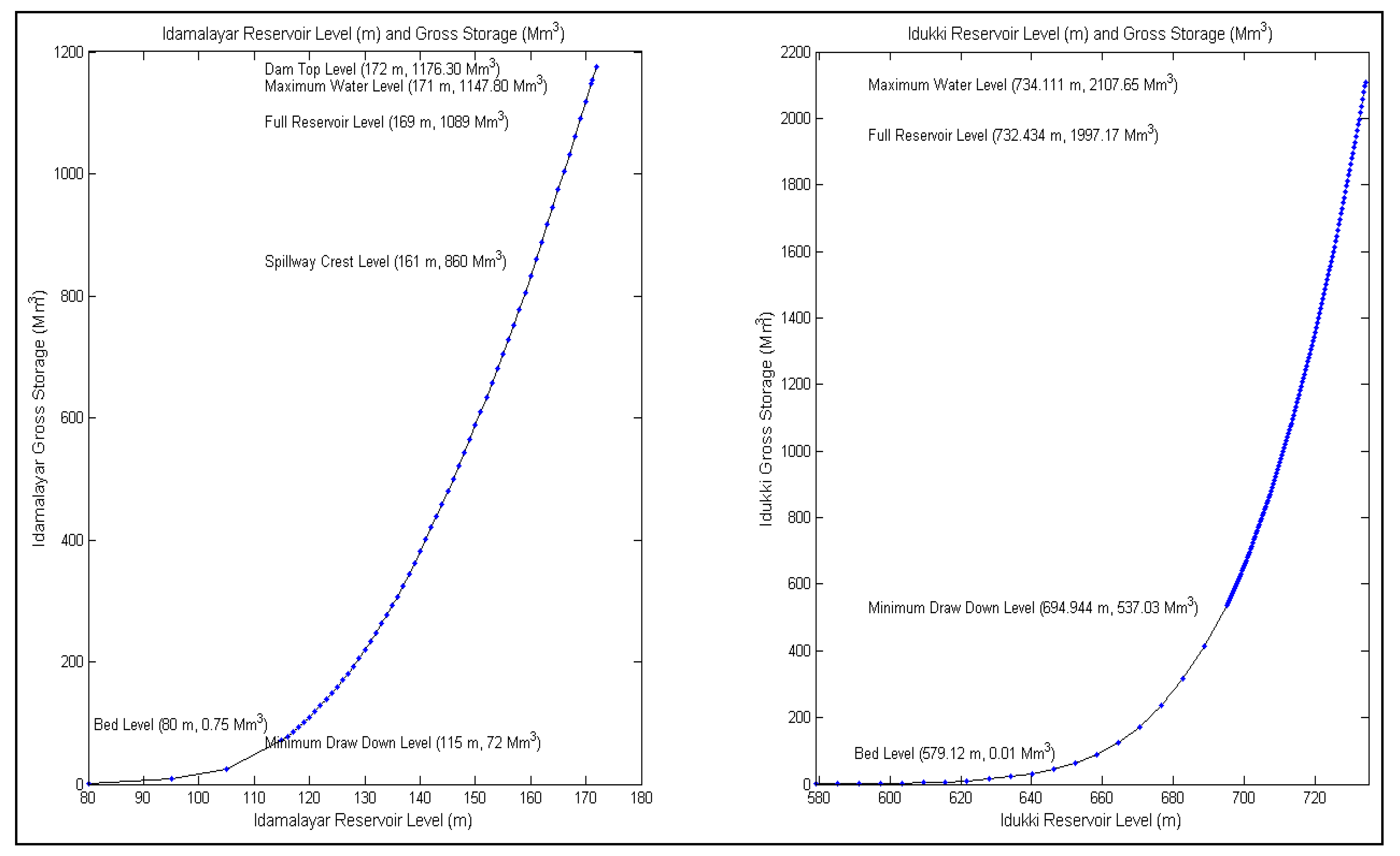
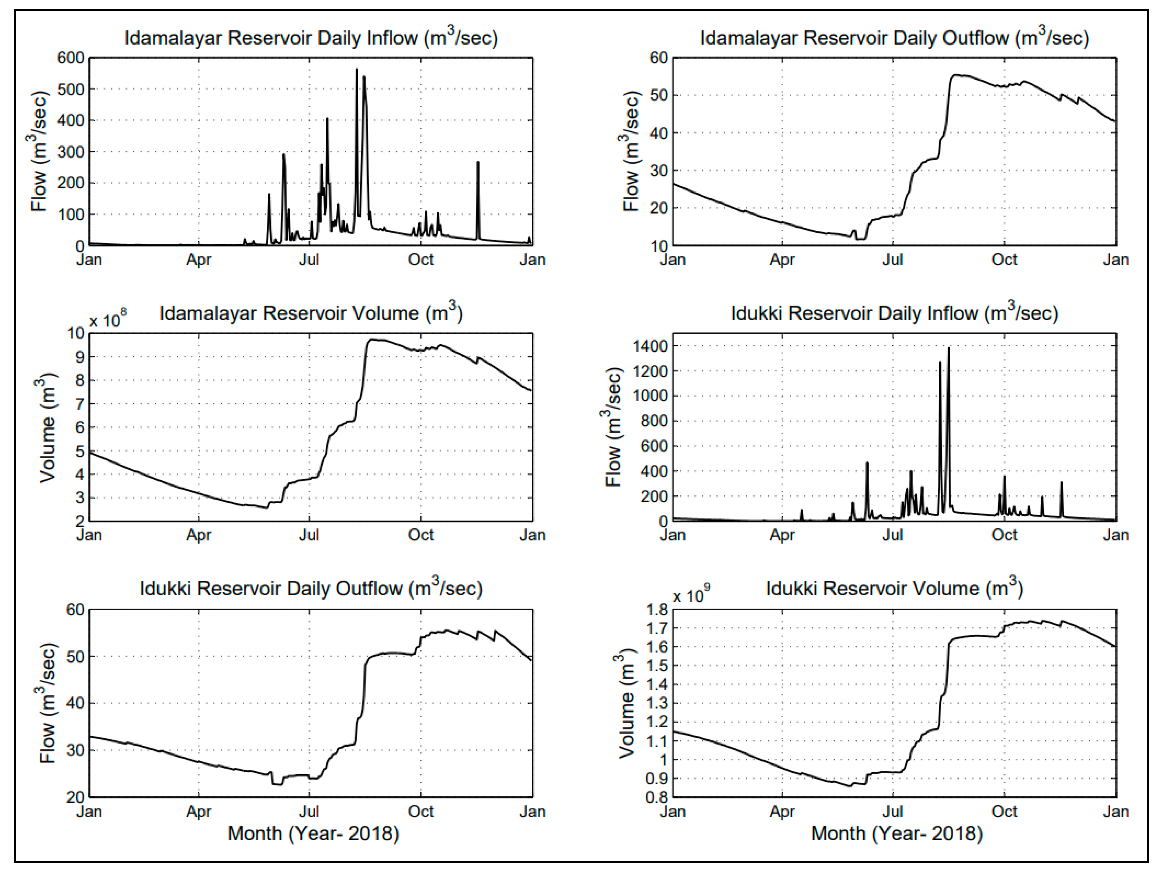
5.2. Reservoir (Idukki and Idamalyar) Rule Curve

5.2.1. Idamalayar Reservoir

The Idamalayar reservoir was created by developing the Ennakkal dam across the Idamalayar river a tributary of Periyar River as part of Idamalayar Hydroelectric Project (75 MW). The reservoir gross storage is 1089.90 Mm3 (Figure 5). The reservoir stored water is diverted through tunneling and penstosks to hydroelectric power station situated on the left bank of Idamalayar River. The power station tailwater is allowed to flow into Idamalayar River. The maximum flood discharge capacity from the reservoir spill way is 3248 cumecs via four numbers of installed radial gates of dimensions 11.50 × 9.70 m. As per the government policy, the rule levels of reservoir are set, i.e., Maximum Water Level (MWL) of reservoir, Full Reservoir Level (FRL), Minimum Draw Down Level (MDDL), and Crest level of spillway, and are 171.20 m, 169.00 m, 115.00 m, and 161.00 m, respectively (Figure 5). At the end of May month, the target level for storage in Idanalyar reservoir is set as 123 m for generating 34 Mu, whereas the target level is set as 168.50 m during the 20 November (end of monsoon season) by the government agencies (Figure 5). The upper rule levels for the period from 1 June to 20 November are arrived at by setting the target level in the reservoir on 20 November as 168.5 m (Figure 6). The target level in the initial time step is taken as 161 m, i.e., the Crest Level of spillway. The target date and level set for lower rule levels are 31 May and 123 m as expressed in Figure 6.

5.2.2. Idukki Reservoir

The Idukki reservoir was created by developing Idukki dam, Cheruthoni dam, and Kulamavu dam as part of Idukki Hydroelectric Project (780 MW). The reservoir gross storage is 1996 Mm3 (Figure 5). The reservoir stored water is diverted to hydroelectric power station situated at Moolamattom. The power station tailwater is allowed to flow into Muvattupuzha river basin. The diversion maximum rate is 147 m3/s (Figure 5). At Cheruthoni dam, reservoir spill way is arranged to flows into the Periyar river through five installed radial gates with dimension 12.19 × 10.36 m. In Idukki reservoir, inflow also comes from adjacent basins, such as Azhutha, Vazhikkadavu, Narakakkanam, Kallar, Erattayar, and Vadakkeppuzha. As per the government policy, the rule levels of reservoir are set, i.e., Dam top Level, MWL of the reservoir, FRL, Crest level of spillway, and MDDL, are 736.09 m, 734.11 m, 732.43 m, 723.29 m, and 694.94 m, respectively (Figure 5). The upper rule levels for the period from 1 June to 20 November are judiciously arrived at by setting the target level in the reservoir on November 20th as 731.52 m (Figure 6). The target level in the initial time step is taken as 723.29 m, i.e., the Crest Level of spillway. Target date and lower rule level set for deriving lower rule levels on 31 May as 704.39 m, as expressed in Figure 6.
Using the above information, the SWAT model was further modified by adding existing reservoir rule curve. The Idamalyar and Idukki reservoir rule levels information, such as dam top level, MWL of reservoir, FRL, MDDL, and Crest level of spillway, was given as input to the SWAT model. After the simulation, the reservoir inflow, outflow, and reservoir storage volume for the year 2018 is plotted on daily basis in Figure 7. The total average volume in the Idamalyar and Idukki reservoir were 584,419,452.1 m3 and 1,264,143,562 m3, respectively, after 998,954,208 m3 and 1,182,194,784 m3 of volume is releases/ use for other purposes, such as hydropower generation for Idamalyar and Idukki dam, respectively.

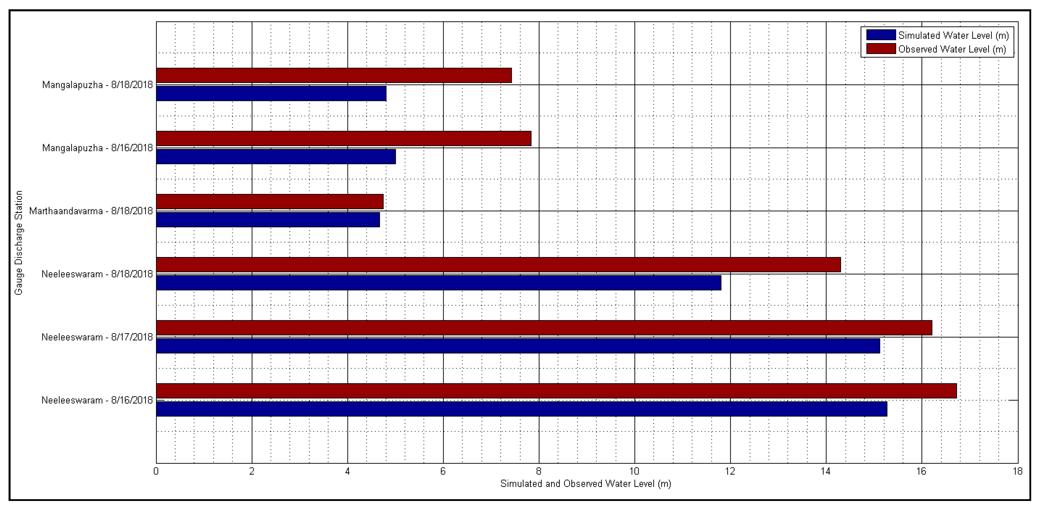
5.3. Calibration and Validation of iRIC Model

The major limitation during the calibration of the iRIC model for flood plain is the potentially distributed bed roughness coefficients ( n ). The Manning’s friction value n was found to be 0.086 during the calibration of iRIC model for the floodplains, which is inside the acceptable range, i.e., 0.05 ≤ n ≤ 0.10 [37]. The output obtained from SWAT model was given as input to iRIC model for simulation. The simulated results from iRIC model were evaluated with the monitored gauge data at the Neeleeswaram, Marthaandavarma, and Mangalapuzha stations. The analysis reported that the iRIC model performance was satisfactory for n = 0.086 (Figure 8).

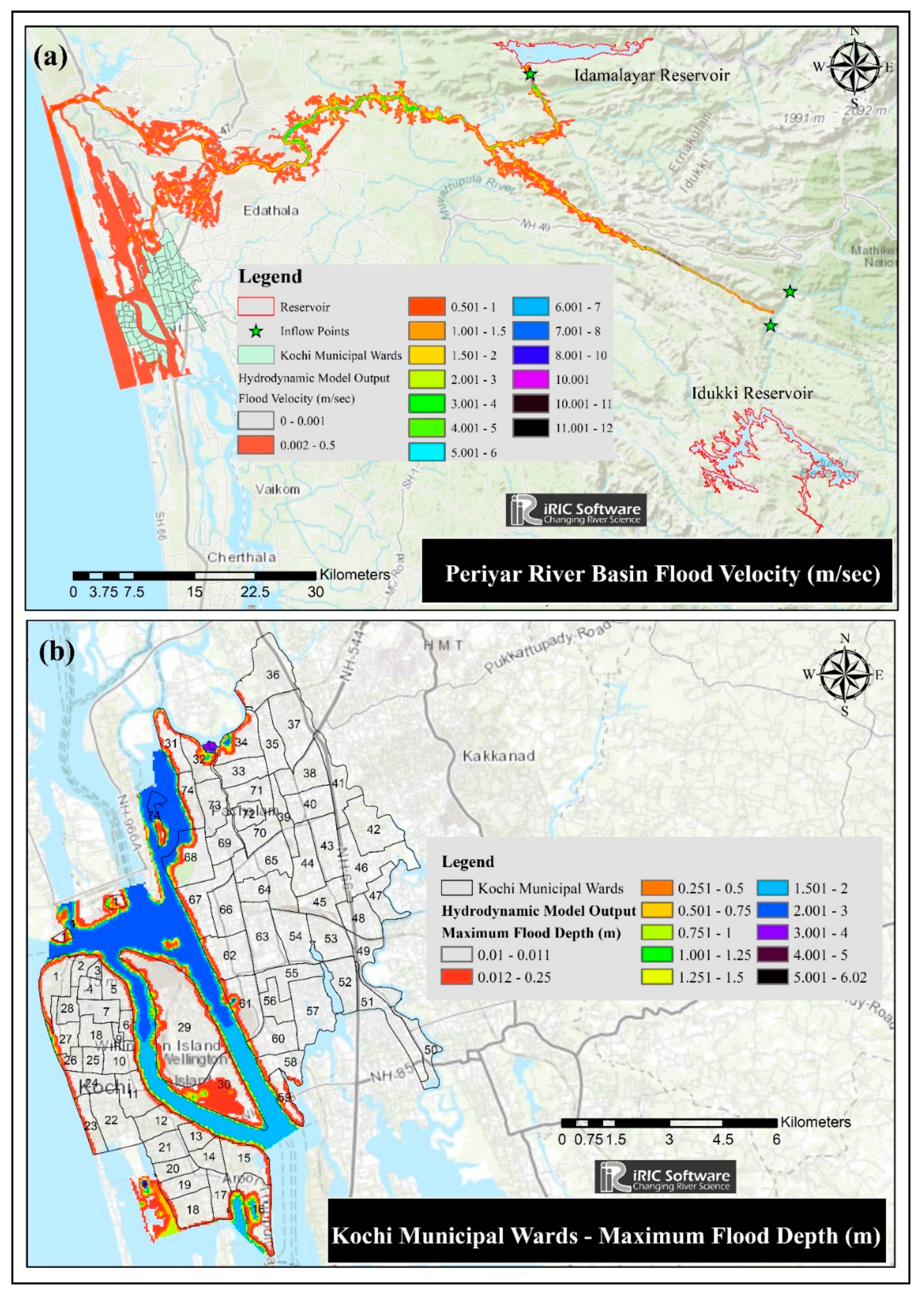
5.4. Coupled Hydrological and Hydrodynamic Model

The iRIC model was applied to the lower reaches of Periyar river basin and its coastal area (Kochi city), which is prone to flood. The performance of the model was in good agreement for flood depth and flood inundation extent. Due to the absence of continuous time series data, the August 2018 flood event was selected for modeling of hybrid model. In the hybrid model, the output from the calibrated SWAT model, outflow from Idamalyar and Idukki reservoir were given as input inflow points into the iRIC (2D) model. To explain the model output, the result is plotted in three different scenarios. The scenarios are: (1) considering reservoir existing rule curve and release from reservoir, (2) considering natural flow conditions without reservoir, and (3) considering reservoir rule curve and downstream rainfall.

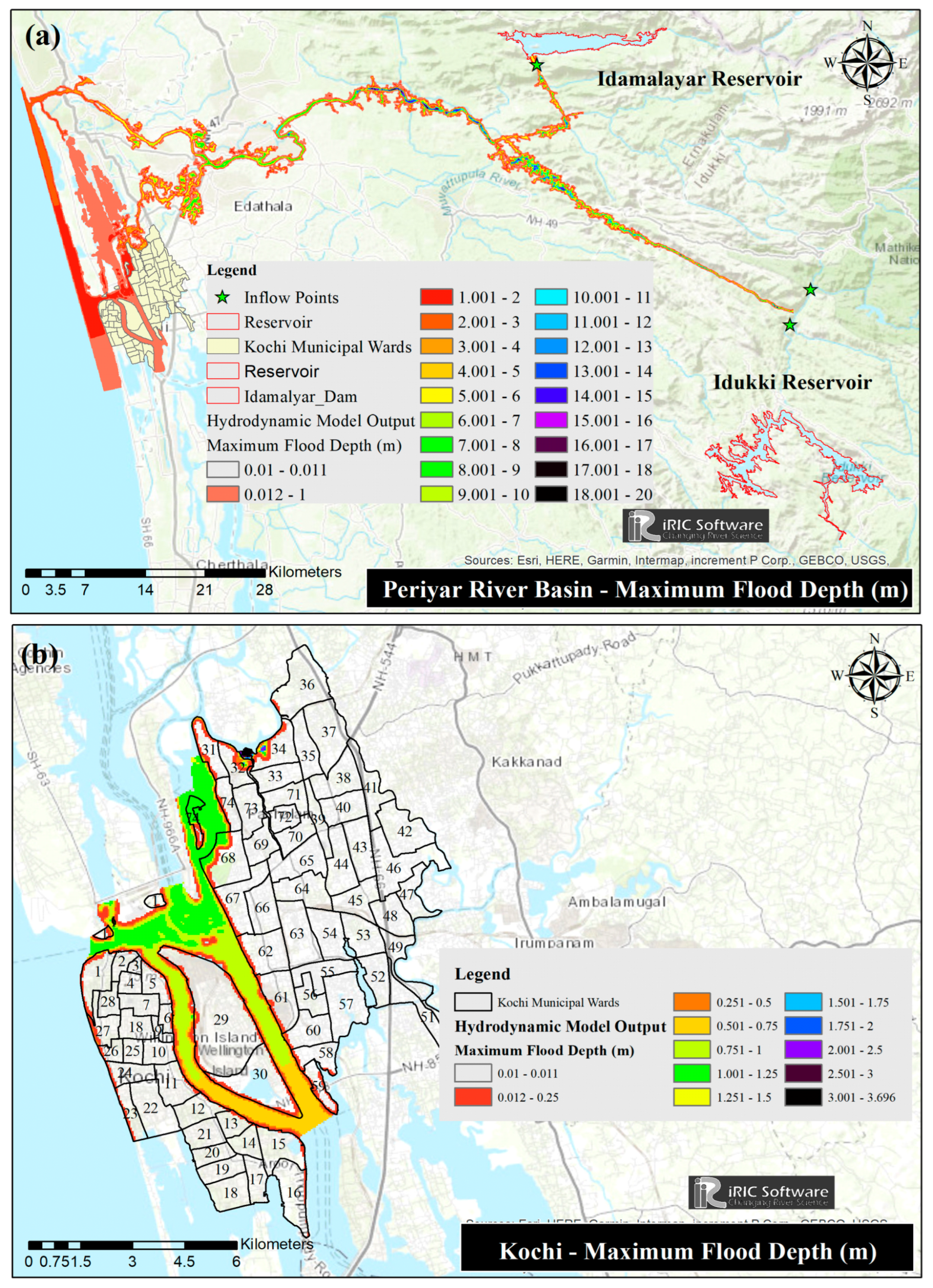
5.4.1. Scenario 1: Considering Reservoir Existing Rule Curve and Release from Reservoir

In Scenario 1, 2D iRIC was developed considering existing reservoir rule curve and outflow from the reservoir as input to the model. Figure 9 explains the flood depth obtained from the hydrodynamic model under controlled conditions. Figure 9a displays the developed 2D hydrodynamic model of Periyar river basin, which includes reservoir operation. Whereas Figure 9b displays the flood water depth in the Periyar river basin ranging from approximately 0.012 m to 3 m. The result is further analyzed using flood water velocity ranging from 0.002–1 m/s in the Periyar river basin (Figure 10a), and flood depth in the Kochi municipal wards level (Figure 10b). It was found that flood water depth in Kochi city was significantly higher ranging from 0.12 m to 3 m.

5.4.2. Scenario 2: Considering Natural Flow Conditions without Reservoir

In Scenario 2, 2D iRIC was developed using natural flow condition without considering reservoir operation. Figure 11 explains the flood depth obtained from the model under natural flow condition. Figure 11a displays the developed 2D hydrodynamic model of Periyar river basin with flood water depth. Whereas Figure 11b displays the flood water depth in Kochi city. The result shows that the flooding depth in Kochi city is less ranging from 0.012 m to 1.5 m whereas in the river basin the depth varies from 0.12 m to 3 m. The reduction in flood depth in Kochi city in the present scenario when compared with Scenario 1 leads to further development of Scenario 3, which will be discussed in the next section.

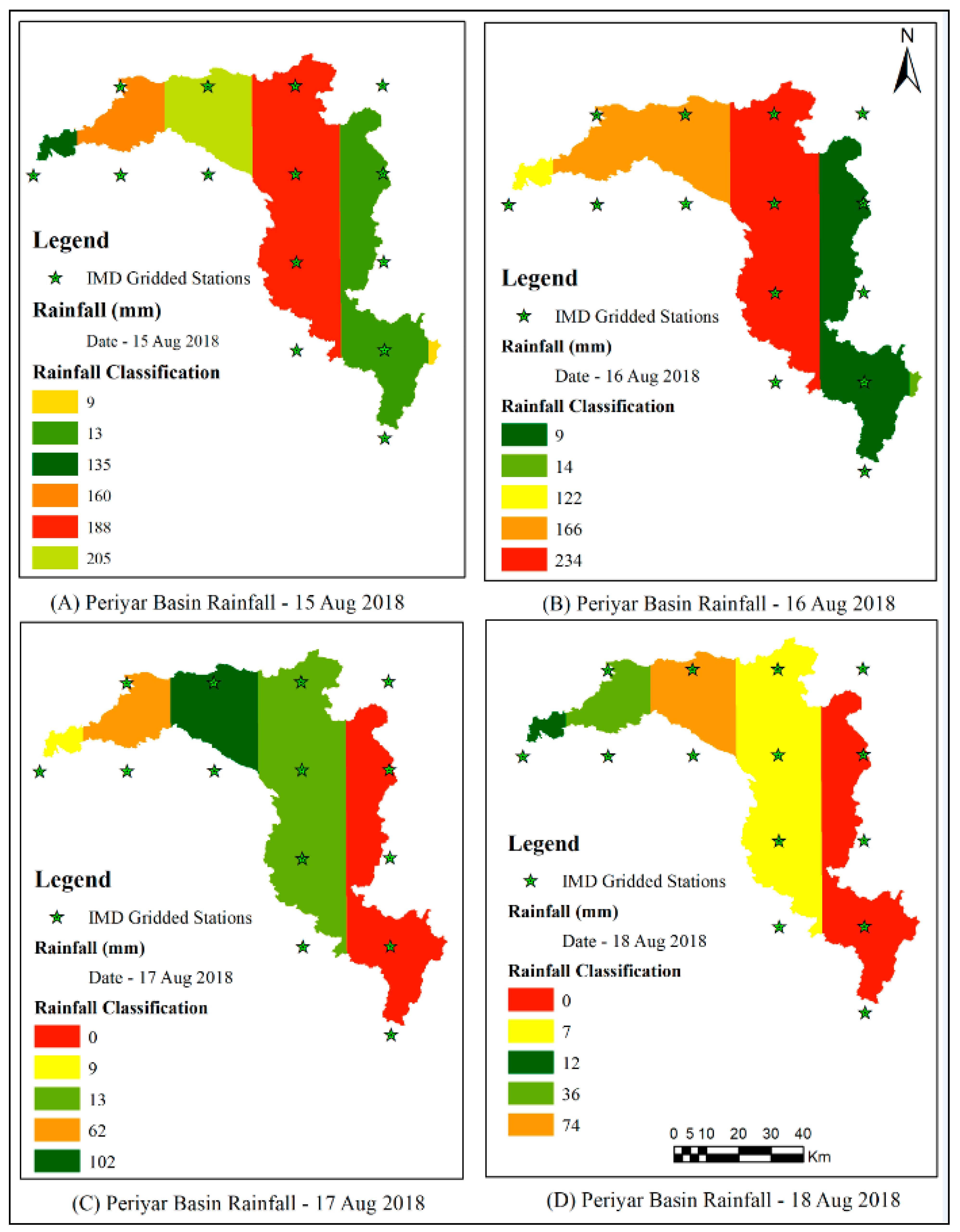
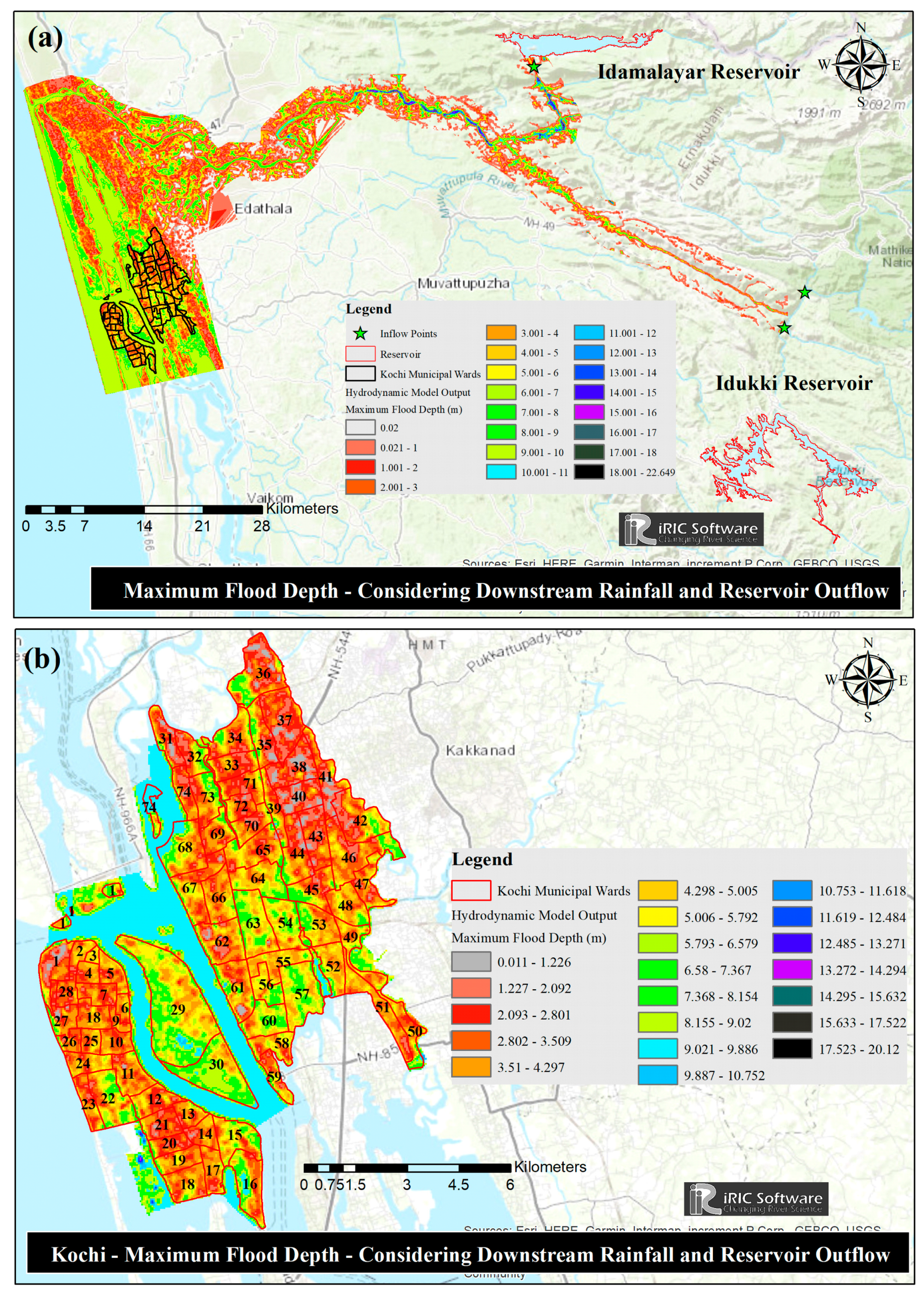
5.4.3. Scenario 3: Considering Reservoir Rule Curve and Downstream Rainfall

In Scenario 3, 2D iRIC was developed considering reservoir rule curve and downstream rainfall near Kochi city. First, the rainfall analysis was completed for Periyar river basin using the precipitation data from 15 to 18 August 2018. The analysis shows that during these four days the rainfall received by the basin is very high from 9 mm to 233.99 mm (Figure 12). Second, when the rainfall is given as input along with the reservoir rule, the model output shows complete inundation of the downstream portion of the basin (Figure 13a). The flood depth varies from 0.02 m to 10 m in the basin. Additionally, when the flooding condition was analyzed in Kochi city, the output shows complete inundation in the city (Figure 13b), where the flood depth varies from 0.011 m to 11 m, which is very high for any city to stop functioning because of this type of flood event.
Further analysis were completed by comparing all the three different scenarios, i.e., (i) natural flow condition, (ii) with reservoir operation, and (iii) considering reservoir and rainfall both have been made for Kochi city, refer to Figure 14. The analysis shows that under natural condition, i.e., without reservoir operation rule curve, the maximum flood depth were around 3.096 m. Results with reservoir operation rule curve, the maximum flood depth were between 5 m to 6 m, whereas when reservoir operation and rainfall both were considered, then the complete city comes under flooding with maximum flood depth varies from 17 m to 20.12 m, which is too high to make any city inundated.
The novelty of the study is to support an integrated flood risk management model in river reservoir system based fluvial models for the urban flooding, particularly in coastal areas, i.e., Kochi city. Thus, providing a significant result to evaluate the occurrence of flood related to its depth, inundated area, and flooding time. This novel framework can deliver on-demand services related to real-time flood forecast using real time hydrometeorological data. The novelties of the proposed model comprise an effective way to link the 1D and 2D models. The 1D, 2D, and coupled models were tested through field data and numerical results validated the accuracy of the models. Furthermore, the coupled 1D–2D model was employed for a real flood simulation in Periyar basin, India. The flood-risk information including flood arrival time and maximal water depth was mapped using GIS. These flood-risk maps can be used as an important decision-making basis of flood control and rescue for the flood control departments at all levels.

6. Conclusions

The main goal of the present study is to evaluate the operation rule of Idamalyar and Idukki reservoir in the Periyar river basin using a hydrological and hydrodynamic modeling approach. For this, a hybrid model (coupled 1D–2D river model) is developed to detect the inundation extent and its flooding depth in the deficiency of continuous time series monitored data. A 2D model, iRIC, was developed under controlled (with reservoir operation policy) and uncontrolled (without reservoir operation policy) conditions for the Periyar river basin of India to check the cause of flooding extent. The performance of the model was reasonably good with the observed field data during the calibration and validation process of the river basin. In the present work, SWAT model was externally coupled iRIC model was developed to evaluate the viability of iRIC model as river flood simulator in Periyar river basin, which has experienced flooding in recent years. The developed SWAT model performed well during calibration and validation stages on a daily basis using the NSE and PBIAS statistical parameters. For explaining the performance of the 2D iRIC model output, three scenarios implemented in the present study, i.e., model under controlled condition, model with uncontrolled condition, and model with controlled condition along with downstream rainfall. The analysis results show that flooding depth is very high in the third scenario, ranging from 0.011 m to 11 m, which may be caused due to the high intensity rainfall. The results match the flooding depth that occurred in Kochi city in the flood year 2018. From the analysis, it is observed that the operation policy of the Idamalyar and Idukki reservoir is well managed as can be seen from Figure 9, Figure 10 and Figure 11, where flooding depth is under 3 m. Thus, the model performances were noted in both flow fields and flood propagations, which is satisfactory. The novelty of this methodology is that the developed framework of coupling the hydrological and hydrodynamic simulation results and final model results can allow flood water movement on the river channel and on the river floodplain. Hence, the temporal evolution of flooding can be defined, and water levels and flow paths can be mapped, which is not present in the simple models. In the present study, only extreme flood events are considered and lean flow conditions are not consider, which are the limitations of the study. However, the analysis can be improved by using long term continuous time series monitored data which will be taken up in future study. The present study offers a valued understanding for operation policy for reservoir in flood reduction at a larger scale. The proposed framework can be utilized as an effective tool for efficient planning and management of natural disasters, such as flash floods.

Author Contributions

Conceptualization, A.K. and R.K.; Methodology, A.K., R.K. and A.K.G.; Software, A.K.; Validation, A.K.; Formal analysis, A.K.; Investigation, A.K.; Resources, A.K., R.K. and A.K.G.; Data curation, A.K. and R.K.; Writing—original draft, A.K.; Writing—review & editing, A.K., R.K. and A.K.G.; Visualization, A.K.; Supervision, R.K. and A.K.G. All authors have read and agreed to the published version of the manuscript.

Funding

This research received no external funding.

Data Availability Statement

The data presented in this study are available on request from the corresponding author.

Conflicts of Interest

The authors declare no conflict of interest.

References

  1. Brakenridge, G.; Anderson, E.; Caquard, S. Dartmouth Flood Observatory. From Dartmouth Flood Observatory. 2005. Available online: http://www.dartmouth.edu/~floods/ (accessed on 24 April 2007).
  2. Brakenridge, G.R.; Anderson, E.K.; Carlos, H. Dartmouth Active Archive of Major Floods. 2009. Available online: http://www.dartmouth.edu/~floods/Archives/index.html (accessed on 10 March 2014).
  3. EM-DAT. The OFDA/CRED International Disaster Database, Version 12.07; Univ. Catholique de Louvain: Brussels, Belgium, 2014; Available online: www.emdat.be (accessed on 26 March 2022).
  4. Di Baldassarre, G.; Montanari, A.; Lins, H.; Koutsoyiannis, D.; Brandimarte, L.; Blöschl, G. Flood fatalities in Africa: From diagnosis to mitigation. Geophys. Res. Lett. 2010, 37, L22402. [Google Scholar] [CrossRef] [Green Version]
  5. Hirsch, R.M.; Ryberg, K.R. Has the magnitude of floods across the USA changed with global CO2 levels? Hydrol. Sci. J. 2012, 57, 1–9. [Google Scholar] [CrossRef]
  6. Kundzewicz, Z.W.; Kanae, S.; Seneviratne, S.I.; Handmer, J.; Nicholls, N.; Peduzzi, P.; Mechler, R.; Bouwer, L.M.; Arnell, N.; Mach, K.; et al. Flood risk and global and regional climate change prospects. Hydrol. Sci. J. 2014, 59, 1–28. [Google Scholar] [CrossRef] [Green Version]
  7. Sewa International. Diaspora, Disaster and Development; Sewa International: New Delhi, India, 2023. [Google Scholar]
  8. National Disaster Management Authority (NDMA), New Delhi. Available online: http://www.ndma.gov.in (accessed on 5 April 2022).
  9. Central Water Commission State-Wide Flood Data Damage Statistics. 2018. Available online: http://cwc.gov.in/sites/default/files/statewiseflooddatadamagestatistics.pdf.33 (accessed on 9 April 2022).
  10. Werner, M. Spatial Flood Extent Modeling—A Performance-Based Comparison. Ph.D. Thesis, Delft University, Delft, The Netherlands, 2004. [Google Scholar]
  11. Bates, P.D.; Lane, S.N.; Ferguson, R.I. (Eds.) Computational Fluid Dynamics: Applications in Environmental Hydraulics; John Wiley & Sons: Hoboken, NJ, USA, 2005. [Google Scholar]
  12. Rai, P.K.; Dhanya, C.T.; Chahar, B.R. Coupling of 1D models (SWAT and SWMM) with 2D model (iRIC) for mapping inundation in Brahmani and Baitarani river delta. Nat. Hazards 2018, 92, 1821–1840. [Google Scholar] [CrossRef]
  13. Kumar, S.; Agarwal, A.; Villuri, V.G.K.; Pasupuleti, S.; Kumar, D.; Kaushal, D.R.; Gosain, A.K.; Bronstert, A.; Sivakumar, B. Constructed wetland management in urban catchments for mitigating floods. Stoch. Environ. Res. Risk Assess. 2021, 35, 2105–2124. [Google Scholar] [CrossRef]
  14. Di Luzio, M.; Arnold, J.G.; Srinivasan, R. Effect of GIS data quality on small watershed stream flow and sediment simulations. Hydrol. Process. Int. J. 2005, 19, 629–650. [Google Scholar] [CrossRef]
  15. Srinivasan, R.; Arnold, J.G. Integration of a Basin-Scale Water Quality Model with GIS. J. Am. Water Resour. Assoc. 1994, 30, 453–462. [Google Scholar] [CrossRef]
  16. Bian, L.; Sun, H.; Blodgett, C.; Egbert, S.; Li, W.; Ran, L.; Koussis, A. An integrated interface system to couple the SWAT model and ARC/INFO. In Proceedings of the 3rd International Conference on Integrating GIS and Environmental Modeling, CD-ROM, US National Center for Geographic Information and Analysis, Santa Fe, NM, USA, 21–25 January 1996. [Google Scholar]
  17. Di Luzio, M.; Srinivasan, R.; Arnold, J.G. An integrated user interface for SWAT using ArcView and Avenue. Trans. Am. Soc. Agric. Eng. 1997, 2, 16. [Google Scholar]
  18. Arnold, J.G.; Srinivasan, R.; Muttiah, R.S.; Williams, J.R. Large area hydrologic modeling and assessment part I: Model development 1. JAWRA J. Am. Water Resour. Assoc. 1998, 34, 73–89. [Google Scholar] [CrossRef]
  19. Neitsch, S.L. Soil and Water Assessment Tool; User’s Manual Version 2005; Texas Water Resources Institute: College Station, TX, USA, 2005; p. 476.
  20. Green, W.H.; Ampt, G.A. Studies on Soil Phyics. J. Agric. Sci. 1911, 4, 1–24. [Google Scholar] [CrossRef] [Green Version]
  21. Boughton, W.C. A review of the USDA SCS curve number method. Soil Res. 1989, 27, 511–523. [Google Scholar] [CrossRef]
  22. Williams, P.J.L. Evidence for the seasonal accumulation of carbon-rich dissolved organic material, its scale in comparison with changes in particulate material and the consequential effect on net CN assimilation ratios. Mar. Chem. 1995, 51, 17–29. [Google Scholar] [CrossRef]
  23. Monteith, J.L. Evaporation and environment. In Symposia of the Society for Experimental Biology; Cambridge University Press (CUP): Cambridge, UK, 1965; Volume 19, pp. 205–234. [Google Scholar]
  24. Hargreaves, G.H.; Samani, Z.A. Reference crop evapotranspiration from temperature. Appl. Eng. Agric. 1985, 1, 96–99. [Google Scholar] [CrossRef]
  25. Priestley, C.H.B.; Taylor, R.J. On the assessment of surface heat flux and evaporation using large-scale parameters. Mon. Weather Rev. 1972, 100, 81–92. [Google Scholar] [CrossRef]
  26. Arnold, D.S.; O’leary, S.G.; Wolff, L.S.; Acker, M.M. The Parenting Scale: A measure of dysfunctional parenting in discipline situations. Psychol. Assess. 1993, 5, 137. [Google Scholar] [CrossRef]
  27. Daniel, J. Sampling Essentials: Practical Guidelines for Making Sampling Choices; Sage Publications: Thousand Oaks, CA, USA, 2011. [Google Scholar]
  28. Borah, D.K.; Bera, M. Watershed-scale hydrologic and nonpoint-source pollution models: Review of mathematical bases. Trans. ASAE 2003, 46, 1553. [Google Scholar] [CrossRef] [Green Version]
  29. Jang, C.L.; Shimizu, Y. Numerical simulation of relatively wide, shallow channels with erodible banks. J. Hydraul. Eng. 2005, 131, 565–575. [Google Scholar] [CrossRef] [Green Version]
  30. Nelson, J.M.; Shimizu, Y.; Abe, T.; Asahi, K.; Gamou, M.; Inoue, T.; Iwasaki, T.; Kakinuma, T.; Kawamura, S.; Kimura, I.; et al. The international river interface cooperative: Public domain flow and morphodynamics software for education and applications. Adv. Water Resour. 2016, 93, 62–74. [Google Scholar] [CrossRef]
  31. Wongsa, S. Simulation of Thailand flood 2011. Int. J. Eng. Technol. 2014, 6, 452. [Google Scholar] [CrossRef] [Green Version]
  32. Moriasi, D.N.; Arnold, J.G.; Van Liew, M.W.; Bingner, R.L.; Harmel, R.D.; Veith, T.L. Model evaluation guidelines for systematic quantification of accuracy in watershed simulations. Trans. ASABE 2007, 50, 885–900. [Google Scholar] [CrossRef]
  33. Fadil, A.; Rhinane, H.; Kaoukaya, A.; Kharchaf, Y.; Bachir, O.A. Hydrologic modeling of the Bouregreg watershed (Morocco) using GIS and SWAT model. J. Geogr. Inf. Syst. 2011, 3, 279. [Google Scholar] [CrossRef] [Green Version]
  34. Nash, J.E.; Sutcliffe, J.V. River flow forecasting through conceptual models part I—A discussion of principles. J. Hydrol. 1970, 10, 282–290. [Google Scholar] [CrossRef]
  35. Gupta, H.V.; Sorooshian, S.; Yapo, P.O. Status of automatic calibration for hydrologic models: Comparison with multilevel expert calibration. J. Hydrol. Eng. 1999, 4, 135–143. [Google Scholar] [CrossRef]
  36. Arnold, J.G.; Fohrer, N. SWAT2000: Current capabilities and research opportunities in applied watershed modelling. Hydrol. Process. Int. J. 2005, 19, 563–572. [Google Scholar] [CrossRef]
  37. Chow, V.T. Open Channel Hydraulics; McGraw-Hill Book Company: New York, NY, USA, 1959. [Google Scholar]
Figure 1. Study Area Showing Basin, Watershed, Reach, River Monitoring Point, and Gauge Discharge Station Locations.
Water 15 01371 g001aWater 15 01371 g001b
Figure 2. Typical procedure layout of the software (http://i-ric.org/en/introduction accessed on 26 August 2022).
Water 15 01371 g002
Figure 3. Periyar river basin where river reaches, reservoirs location, and gauging stations is shown in (A), Land use (B), Soil (C), and Slope (D).
Water 15 01371 g003
Figure 4. Observed and simulated daily and monthly streamflow’s at the Neeleshwaram and Kalady gauging stations during the calibration and the validation periods.
Water 15 01371 g004
Figure 5. Idamalyar and Idukki level and gross storage relationship.
Water 15 01371 g005
Figure 6. Idamalyar and Idukki available lower and upper rule curve.
Water 15 01371 g006
Figure 7. Reservoir Inflow, Outflow and storage plot considering reservoir operation.
Water 15 01371 g007
Figure 8. iRIC model calibration at Neeleeswaram (16–18 August 2018), Marthaandavarma (18 August 2018), and Mangalapuzha (16 and 18 August 2018).
Water 15 01371 g008
Figure 9. Hydrodynamic model flood depth output of Periyar river basin under controlled flow condition (with reservoir operation) where (a) shows the maximum flood depth in Periyar River Basin and (b) shows maximum flood water depth in the Periyar River basin.
Water 15 01371 g009
Figure 10. Hydrodynamic model flood depth output of Kochi city and flood velocity of Periyar river basin under controlled flow condition (with reservoir operation) where (a) shows the flood velocity in Periyar River Basin and (b) shows maximum flood depth in the Kochi Municipal.
Water 15 01371 g010
Figure 11. Hydrodynamic model flood depth output of Kochi city and Periyar river basin under natural flow condition (without reservoir operation) where (a) shows the maximum flood depth in Periyar River Basin and (b) shows maximum flood depth in the Kochi City.
Water 15 01371 g011
Figure 12. Rainfall analysis of Periyar river basin (15–18 August 2018).
Water 15 01371 g012
Figure 13. Hydrodynamic model flood depth output of Kochi city and Periyar river basin under Controlled Flow Condition (with reservoir) considering downstream rainfall where (a) shows complete inundation of the downstream portion of the basin and (b) shows complete inundation in the Kochi city.
Water 15 01371 g013
Figure 14. Comparison of Kochi City Maximum Flood Depth at three Different Scenarios, i.e., (i) Natural Flow Condition, (ii) With Reservoir Operation, and (iii) Considering Reservoir and Rainfall Both.
Water 15 01371 g014
Table 1. SWAT model parameters, process, their description, parameter ranges, default value, and fitted value in the stepwise calibration process.
Sr. No.ParameterProcessDescription UnitRange (Min–Max)SWAT Default ValueFitted Value
1CN2.mgtSurface runoffSCS runoff curve number for moisture condition II-30–98 Changes for HRU50–80 (Varies by HRU)
2ALPHA_BF.gwGroundwaterBaseflow alpha factor (d−1)-0–10.0480.036
3GWQMN.gwGroundwaterThreshold depth of water in the shallow aquifer required for return flow to occurmm H2O0–500001150
4GW_REVAP.gwGroundwaterGroundwater ‘revap’ coefficient-0–50010.09
5CH_N2.rteSurface runoff (Channel)Manning’s ‘n’ value for main Channel-−0.01–0.30.0140.017
6ESCO. HruSurface runoff (HRU)Soil Evaporation Compensation Factor-0–10.950.78
7GW DELAY.gwGroundwaterGround Water Delay Timedays0–5003138
8SOL AWC. SolSurface runoffAvailable Water Capacitymm H2O/mm soil0–1-0.26
9EPCO.bsnSurface runoff (hru)Plant uptake compensation factor-0–100.11
10RES_K.resReservoirHydraulic conductivity of reservoir bottomMm/h0.1–11.4-2.1
11SURLAG. BsnSurface runoffSurface runoff lag timedays1–2444.19
12SHALLST.gwGroundwaterInitial depth of water in the shallow aquifermm H2O0–10000.50.65
Table 2. NSE and PBIAS values during calibration and validation.
Station NameDaily CalibrationDaily ValidationMonthly CalibrationMonthly Validation
NSEPBIASNSEPBIASNSEPBIASNSEPBIAS
Neeleeshwaram0.58817.070.51419.3540.76721.1030.63223.175
Kalady0.53821.0230.61920.6560.64224.6380.75212.771
Disclaimer/Publisher’s Note: The statements, opinions and data contained in all publications are solely those of the individual author(s) and contributor(s) and not of MDPI and/or the editor(s). MDPI and/or the editor(s) disclaim responsibility for any injury to people or property resulting from any ideas, methods, instructions or products referred to in the content.

