Abstract
Soil moisture is a critical variable in the hydrological cycle and the climate system, significantly impacting water resources, ecosystem functioning, and the occurrence of extreme events. However, soil moisture data are often scarce, and soil water dynamics are not fully understood in mountainous regions such as the tropical Andes of Ecuador. This study aims to model and predict soil moisture dynamics using in situ-collected hydrometeorological data for training and data-driven machine-learning techniques. Our results highlight the fundamental role of vegetation in controlling soil moisture dynamics and significant differences in soil water balance related to vegetation types and topography. A baseline model was developed to predict soil moisture dynamics using neural network techniques. Subsequently, by employing transfer-learning techniques, this model was effectively applied to different soil horizons and profiles, demonstrating its generalization capacity and adaptability. The use of neural network schemes and knowledge transfer techniques allowed us to develop predictive models for soil moisture trained on in situ-collected hydrometeorological data. The transfer-learning technique, which leveraged the knowledge from a pre-trained model to a model with a similar domain, yielded results with errors on the order of . For the training data, the forecast of the base network demonstrated excellent results, with the lowest magnitude error metric RMSE equal to , and NSE and KGE both equal to 0.97. These models show promising potential to accurately predict short-term soil moisture dynamics with potential applications for natural hazard monitoring in mountainous regions.
1. Introduction
Soil moisture is a key variable in the climate system, as well as in water, energy, and biogeochemical cycles [1,2]. Better quantification of the spatiotemporal variability in soil moisture contributes to reducing uncertainty in climate change modeling, particularly with respect to the occurrence and frequency of extreme weather events such as droughts or long continuous periods of rain [3]. Moreover, soil moisture dynamics also play a key role in predicting the potential impact of weather events on, e.g., fires, floods, and landslides, and on soil productivity and ecosystems as described in [4]. Despite its importance, soil moisture is one of the least understood and most difficult variables to measure in the field of soil hydrology [5]. Moreover, vegetation plays a fundamental role in soil moisture at different spatial and temporal scales, as plants extract water from the soil and influence water pathways and flows [6,7].
The Andean páramo ecosystem is found in the high tropical Andes and is characterized by a glacially sculpted morphology with presence of tussock grasses, cushion-forming plants, and patches of Polylepis forest [8]. Soil moisture dynamics in páramo ecosystems are of great interest for future planning of water resources in the Andean region [9,10]. The páramo environment is characterized by low physical erosion rates [11] and sustained rainfall input throughout the year [12], and soils formed from volcanic ash accumulation contain high organic matter content (i.e., up to more than 50%, [13]) and have high-water retention and infiltration capacities [14]. Soil moisture dynamics are controlled by prior moisture content and atmospheric conditions, and they affect the hydrological connectivity and functioning of high Andean watersheds [7,15]. Topography, soil physicochemical properties, and vegetation cover further control the hydrology of the Andean páramo [16]. Previous studies on soil hydrology in the region have been predominantly realized in areas with shallow soils that overlie volcanic or metasedimentary parent material. This includes work by, e.g., Iñiguez et al. [17] and Patiño et al. [9], on the hydrological response of páramo soils to extreme rainfall and drought. Deep polygenetic volcanic soils have been less studied although they are prevalent in the northern and central part of Ecuador [10].
Soil moisture dynamics control surface runoff generation, but rainfall-runoff responses are not yet fully understood [18]. Few empirical studies have analyzed the rainfall-runoff response in Andean ecosystems. Previous work by, e.g., Molina et al. [19], mainly focused on agri-environmental systems in the inter-Andean region and used rainfall simulation experiments to examine the hydrological response of different soil types and vegetation covers. These authors [20] demonstrated that the hydrological response can be highly variable in space and time and is directly linked to soil moisture dynamics.
Given the importance of the high Andes for providing hydrological services for the developing urban centers in the inter-Andean valleys, there is growing interest in modeling and forecasting soil moisture dynamics based on hydrometeorological variables [15]. In situ-collected soil moisture data are increasingly available for high Andean sites [7,17,21], and it would be of utmost importance to include these observations in a data-driven model for soil moisture forecasting, which would improve environmental monitoring and water resource management during extreme weather events [22]. Such data-driven approaches complement physically based and deterministic approaches that are often limited by the large number of observed environmental variables that are not always available, as shown by Prasad et al. [22].
Research on applied agri-environmental modeling has used machine learning techniques for soil moisture forecasting including neural network schemes, such as deep long short-term memory and convolutional neural networks [23,24]. These networks utilized hydro-meteorological variables as input data. In Suebsombut et al. [25], a similar approach was employed to predict soil moisture based on environmental parameters collected from various smart sensors, with the aim of enhancing crop irrigation. Other work by Sivasankaran et al. [26] developed predictive models for soil moisture employing a generative adversarial network in conjunction with a Sailfis optimization algorithm. In Liu et al. [27], an artificial neural network was constructed using a backpropagation optimization method in combination with a genetic algorithm for the prediction of soil moisture variations on sloping land, and Zhang et al. [28] estimated soil moisture variations using an enhanced generalized regression neural network for a high mountainous site located in the Tibet Autonomous Region.
Soil moisture prediction based on machine-learning techniques trained by in situ-collected data of rainfall and hydrometeorological variables [29] has great potential for forecasting soil water dynamics and also the impacts of extreme events such as agricultural drought, runoff generation, and pluvial flooding. Furthermore, it can facilitate the assessment of water quality impacts during prolonged rainy seasons, primarily as a result of antecedent rainfall [30]. In mountainous terrain, accurate soil moisture forecasting can improve mass movement susceptibility prediction, as soil moisture dynamics play an essential role in slope stability [31]. Accurate soil moisture forecasting can contribute to better prediction and forecasting of mass movements and fires, and they can feed into early warning systems for natural hazards [32].
This study addresses the spatiotemporal patterns in soil moisture dynamics in the high tropical Andes and analyzes how data-driven machine-learning techniques, such as neural networks, can be effectively utilized to predict soil moisture dynamics using hydrometeorological and soil hydrological variables recorded in the field. In addition, it explores how knowledge transfer from previously trained models can enhance the accuracy of soil moisture prediction at various monitoring points within high mountain regions. This study was conducted in a high-elevation Andean catchment, Jatunhuayco, characterized by Holocene volcanic activity and deep polygenetic volcanic soils. In these environments, rainfall is highly heterogeneous, even over small distances, as shown in Ruiz et al. [12]. The study area is part of the Antisana’s Water Conservation Area, which provides water to Quito, Ecuador’s capital. Previous research showed that soil moisture dynamics vary with soil properties and vegetation cover [7,33] and that hydrological conditions can vary at short distances as a result of pedological and lithological diversity [34]. Applying advanced models for soil moisture prediction in a challenging geographical environment can yield results that may be informative for water resource management and the mitigation of impacts of extreme climatic events within these regions.
2. Study Area
The studied sites are situated within JTU_01 sub-basin, which spans an area of 0.7 km2, located on the western slopes of the Antisana volcano in the Northern Andes of Ecuador, within the Antisana Water Conservation Area. Its elevation ranges from 4083 to 4279 m.a.s.l. and the slopes fluctuate from 10 to 22% [7,33]. The sub-basin Figure 1a is ecologically and hydrologically well monitored and forms part of the páramo ecosystem within the La Mica Quito Sur system. This system is a crucial water source for more than half a million inhabitants of the Metropolitan District of Quito [35]. The area is managed by the city’s Water Protection Fund (FONAG) [36]. Since 2011, anthropogenic activities and extensive grazing have been prohibited to preserve the ecosystem.
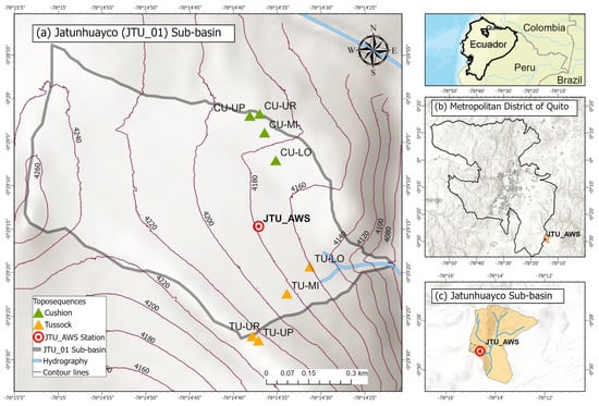
Figure 1.
Location of the study area in the northern Ecuadorian Andes. (a) Study area with location of the soil profiles. (b) Location of the study site in the Metropolitan District of Quito. (c) Location of the study area, JTU_01, within the Jatunhuayco catchment.
To better understand the soil hydrology in young volcanic ash soils, two experimental hillslopes at JTU_01 were implemented and monitored. JTU_01 was equipped in the scope of the páramoSUS project, a joint collaboration effort between Ecuadorian and Belgian academic institutions, EPMAPS-Q, and FONAG. The monitored hillslopes differ only in their dominant vegetation cover. One is dominated by tussock grasses (Calamagrostis intermedia) and the other by cushion plants (Azorella pedunculata). Each hillslope consisted of four soil water sampling positions, upper (UP), upper replica (UR), middle (MI), and lower (LO). A total of eight soil profiles were excavated along the two toposequences. Four soil horizons (A, 2A, 2BC, and 3BC) were identified in the upper part of each profile. The upper A and 2A horizons were analyzed in this study. The toposequences of the two types of analyzed vegetation cover, with consideration to the contour lines, can be seen in Figure 1a and in more detail in Páez-Bimos et al. [33].
At the JTU_AWS meteorological station (Figure 1a), meteorological variables were recorded between 16 October 2018 and 7 October 2022 The mean annual average precipitation was 2.1 mmd−1, the air temperature was 4.12 °C, the incoming solar radiation was 138.01 Wm−2, and the relative humidity was 93.72%. The rooting depth reached 70 cm in the TU-UP and 30 cm in the CU-UR profiles. The soils in the upper meter are polygenetic vitric Andosols developed on Holocene volcanic deposits [37]. These soils overlie a sequence of paleosols and tephra layers approximately 27 m thick, which are situated atop strata rich in scoria and glaciofluvial sediments [38].
3. Methodology
3.1. Data Collection
Table 1 displays the location and description of the soil profiles analyzed within the Jatunhuayco sub-basin, with the two predominant vegetation covers, Azorella pedunculata (CU-Cushion) and Calamagrostis intermedia (TU-Tussock) being considered. The table includes the location, altitude, and slope gradient of the soil profile; the dominant vegetation cover; and the depth of the two upper horizons (A and 2A). Three time-domain reflectometers (CS650, Campbell Scientific, Logan, UT, USA) were installed in each soil profile to measure volumetric water content () and soil temperature (T). The reflectometers were duly calibrated using soil monoliths, and the calibration equations were established for the different horizons. The accuracy of volumetric water content readings was , owing to soil-specific calibration conducted at the LEMSUR laboratory of Escuela Politécnica Nacional [7].

Table 1.
Location of the soil profiles, with description of the main site characteristics.
Table 2 summarizes the meteorological variables that were used in this study and provides information on the environmental sensors used to measure precipitation, air temperature, relative humidity, and solar radiation in the automatic weather station, JTU_AWS. The environmental variables were automatically recorded at a 5 min interval over a period close to 4 years, from 16 October 2018 to 7 October 2022. Table 2 mentions the accuracy and measurement range of the variables. The meteorological information was validated following the methodology outlined in [7].

Table 2.
Information about the variables recorded at the JTU_AWS station from 16 October 2018 to 7 October 2022 with a recording frequency of 5 min.
The hydrometeorological and ancillary environmental data were used as input to forecast soil moisture. Figure 2 illustrates the overall methodological framework of the neural network architecture and includes information on the training, validation, and evaluation datasets. Transfer-learning techniques were implemented to transfer knowledge from a specific domain to another, similar to was done in Zhuang et al. [39]. As such, the knowledge learned from the base network for, e.g., forecasting soil moisture in the lower part of the A-horizon () under cushion vegetation, was then applied to forecast soil moisture at other depths and in other sites covered by tussock grasses and cushion vegetation with a similar domain.
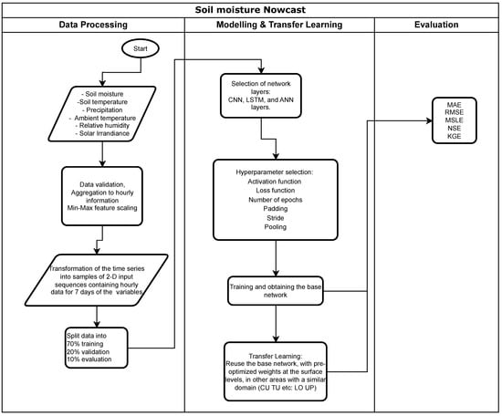
Figure 2.
Flowchart for soil moisture forecasting using neural networks.
3.2. Descriptive Analysis of Variables and Data Preprocessing
At this stage, a detailed analysis of the variables used in the study was conducted, along with the preprocessing necessary for the subsequent application of neural networks. An exhaustive descriptive analysis was carried out, including visual and statistical analysis procedures to understand the nature and distribution of the data. Violin plot graphs were generated to visualize the variables’ distribution. Additionally, descriptive statistics such as mean, standard deviation, percentiles, and other relevant indicators were calculated to provide an overview of the characteristics and spatiotemporal variabilities present in the collected data.
3.3. Artificial Neural Network Models
3.3.1. The Multilayer Perceptron
The multilayer perceptron, or artificial neural network, simulates biological neurons as computational devices [40]. According to Kelleher et al. [41], a neuron is the simplest unit, and a group of aligned neurons forms a layer. Neurons and layers are connected by assigning them a weight w and an activation function f, turning the neural network into a multiple-input linear regression function [41]. The network is analytically represented as the mapping , where represents optimized hyperparameters such as the number of neurons, hidden layers, activation functions, and weights, with the aim of finding the closest representation of the target variable given a set of inputs [42]. Visually, this is shown in Figure 3.
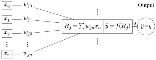
Figure 3.
Basic representation of a neural network.
3.3.2. Convolutional Neural Networks
Convolutional neural networks (CNNs) are specialized for processing data with mesh-like topology and are commonly used in computer-vision tasks such image recognition [42]. The convolution operation is defined as for 1-D inputs and for 2-D inputs, where is the input, and is the kernel. CNNs utilize a kernel (filter) sliding over input values to perform operations, producing a feature map [40]. Goodfellow et al. [42] mention that CNNs include pooling or detection layers, using statistical functions such as mean, maximum, or minimum for internal representations of specific inputs, as illustrated in Figure 4.
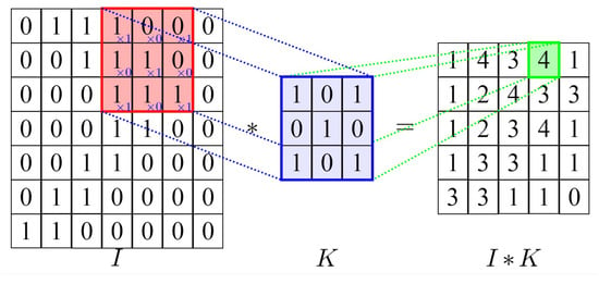
Figure 4.
Two-dimensional representation of a convolution. The kernel’s sliding or stride K is one step over the input matrix I. The result I*K is the feature map, i.e., the element-wise product of elements.
3.3.3. Long Short-Term Memory Networks
According to Sit et al. [43], long short-term memory networks (LSTMs) address the vanishing gradient problem and consist of a state and three “gates”: forget, input, and output. Before passing through the gates, the input value is combined with the previous neuron value into a vector v. The forget gate consists of the vector v and a sigmoid function , resulting in . The input gate is composed of the vector v, a sigmoid function , and a hyperbolic tangent function , resulting in . The state is obtained using , , , and , resulting in . Finally, the output gate is obtained using the vector v, , and , resulting in , as shown in Figure 5.
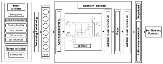
Figure 5.
Neural network architecture: soil moisture forecast for the next 48 h based on information of the preceding 7 days. Base network developed for soil profile under cushion-forming plants in the footslope position of the soil catena ().
3.3.4. Transfer Learning
Transfer learning utilizes pre-trained structures, reducing the resources and time for training new models. It aims to enhance accuracy by leveraging knowledge across related domains [39]. It also prevents issues such as overfitting by generalizing useful features [44]. Deep transfer learning explores knowledge usage through neural networks and has four categories: instance-based, mapping-based, network-based, and adversarial-based [44]. This work employed network-based transfer learning, reusing pre-trained neural networks across different domains to improve performance.
3.4. Design and Implementation of Neural Network Architecture
3.4.1. Data Preprocessing
During the data preprocessing steps, one of the commonly used techniques is data normalization, which is carried out using the following equation:
where X is the original variable, is the minimum value of X, and is the maximum value of X. This operation scales the values of X in the range between 0 and 1. The neural network that was developed for soil moisture forecasting (Figure 5) consists of a deep architecture that leverages the features of convolutional neural networks, long short-term memory networks, and artificial neural networks. The advantage of combining these networks is the utilization of new representations generated by the convolutional layers, the learning from the temporal patterns captured by long short-term memory layers, and the approximation of soil moisture values through the generalized mapping of artificial neural network layers. Moreover, to perform operations only within the temporal segment of the data and avoid random interactions between different time steps and channels, a temporally distributed wrapper was used. This wrapper is applied over another layer in the neural network, enabling the sharing of the long short-term memory layer’s parameters across all time steps. This aids the neural network in processing sequences of varying lengths more efficiently and effectively [43].
3.4.2. Setup of the Base Neural Network and Deep Transfer Learning
For the development of the base network and its architecture, we randomly selected one of the sites for which empirical data on soil moisture were available, i.e., the soil profile located at the footslope position in the soil catena under cushion-forming plants [33]. As all sites had excellent data coverage in the experimental site, any site could have been considered for the construction of the base model. The network forecasted soil moisture for the next 48 h based on hourly records of P, T, , , and , as well as soil moisture data of the preceding seven days; see Figure 5.
Once the model was trained, the base network for forecasting was obtained. Subsequently, network-based deep transfer learning was employed, which involved reusing the network with already optimized weights at the surface levels to train it with information from deeper levels; see Figure 6. This process enabled the prediction of soil moisture in deeper soil horizons (A and 2A) and in other topographic positions (LO, MI, UP, UPR) and vegetation covers (CU, TU). For instance, the base network trained for soil moisture forecasting under cushion-forming plants, , was then used to inform the network forecasting soil moisture in the 2A horizon of the soils at the top slope position under tussock grasses, .
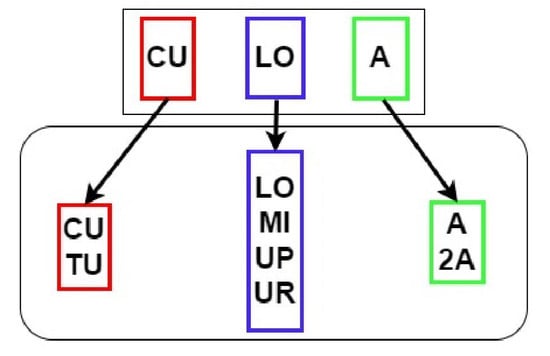
Figure 6.
Transfer learning for similar domains showing the transfer of knowledge for forecasting soil moisture under 15 different conditions. The codes refer to different types of vegetation cover (CU = cushion-forming plants; TU = tussock grasses), topographic position (LO = footslope; MI = mid-slope; UP = top slope; UPR = replica at top slope position) and soil horizon (A and 2A).
3.5. Training of the Network Hyperparameters
During the training process, the following adjustments were made to crucial hyperparameters to ensure optimal performance of the neural network. With regard to the activation functions, the rectifier linear unit function, hyperbolic tangent, and sigmoid or logistic functions were used.
The rectifier linear unit function (ReLU)
was chosen for its capability to allow output of positive values, effectively mitigating the vanishing gradient problem and facilitating quicker convergence during training. To confine the output between −1 and 1, the hyperbolic tangent function (tanh) was used, as the tanh function
offers smooth gradients and aids convergence, which is particularly suitable for the data distributions of our hydrometeorological data.The sigmoid or logistic function,
operating within a range of 0 to 1 is commonly employed for binary classification tasks and allowed us to squash the input values to a probabilistic range.
For the loss function and the evaluation of the model’s performance, mean squared error (MSE) was employed. The MSE
quantifies the average squared difference between predicted () and observed () values and provides a comprehensive measure of model performance.
The adaptive learning rate optimization algorithm (ADAM) was employed to optimize network weights with the following parameters:
where and represent exponential decay rates for the first and second moment estimates, and ensures numerical stability.
In addition, the model uniformly applied padding around the input data to maintain the spatial dimensions of the convolutional layers. Ensuring consistent output dimensions is particularly vital in preserving the feature map size post-convolution. The stride represents the movement of the filter window across the input data during convolution. A stride of (3, 3) was used here as to allow a three-pixel horizontal and vertical movement, influencing subsequent layer output dimensions.
To reduce computational complexity while retaining the essential information, feature maps were downsampled using pooling. Here, we applied a pooling size of (2, 2), implying a downsampling by a 2 × 2 window, with the maximum or average value being selected so as to reduce spatial dimensions but preserve the significant features.
3.6. Model Performance Measures
To assess the performance of the forecasting models for soil moisture (), we used five evaluation metrics to gain insights into the accuracy and reliability of the model predictions. Here, we list five widely adopted performance measures with their descriptions:
- Mean absolute error (MAE): Measures the average absolute difference between predicted () and observed () values.
- Root mean squared error (RMSE): Provides an estimate of the standard deviation of the residuals, indicating the average magnitude of error.
- Mean squared logarithmic error (MSLE): Similar to MSE but particularly useful when target variables vary over several orders of magnitude.
- Nash–Sutcliffe efficiency (NSE): Measures the predictive power of the model by comparing the squared differences between the observed and predicted values with the squared differences between the observed and mean values.
- Kling–Gupta Efficiency (KGE): An index that combines correlation, bias ratio, and variability ratio to evaluate overall model performance.where r is the correlation coefficient, s is the ratio of the standard deviation of simulated to observed values, and b is the ratio of the mean of simulated to observed values.
These metrics and their corresponding equations offered a comprehensive means of assessing model performance in predicting soil moisture levels.
4. Results
4.1. Observational Data on Weather, Soil Temperature, and Moisture
4.1.1. Descriptive Analysis in Weather Data
The automatic weather station JTU_AWS (see Figure 1) has been collecting meteorological data at a five-minute frequency since 2018 for the following variables: precipitation, air temperature, relative humidity, solar radiation, barometric pressure, wind speed, and wind direction. In Figure 7, the violin plots provide insight into the frequency distribution of the analyzed variables.
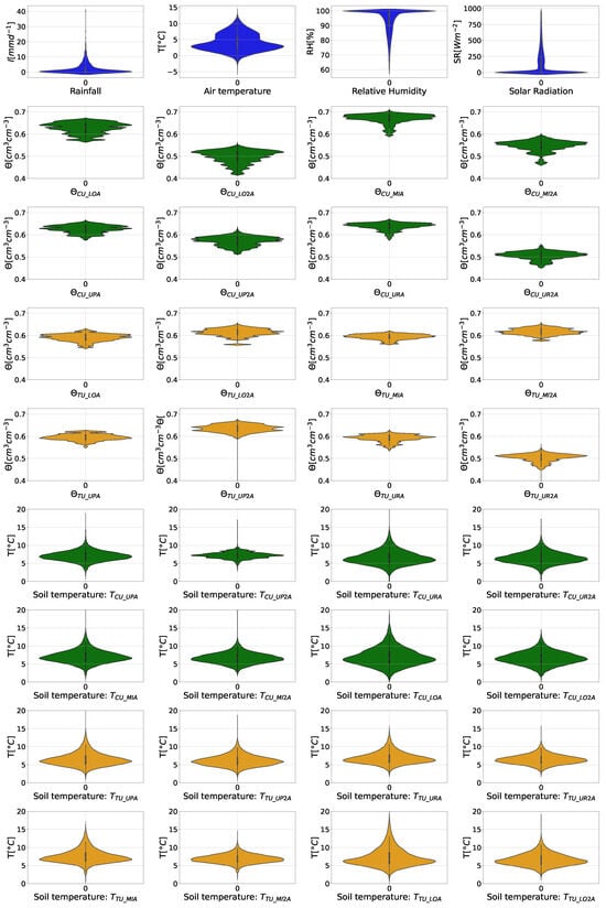
Figure 7.
Violin plots of meteorological variables at the JTU_AWS station and soil variables at Jatunhuayco JTU_01.
4.1.2. Descriptive Analysis of Soil Temperature
For a brief description of the soil temperature in horizons A and of the two soil types, Azorella pedunculata and Calamagrostis intermedia, in the analyzed profiles of UP, UR, MI, and LOm Table 3 and Table 4 are presented, along with violin plots in rows 6 to 9 of Figure 7, illustrating the behavior of this variable.

Table 3.
Statistical description of soil temperature (°C) in profiles A and 2A, for the cushion vegetation.

Table 4.
Statistical description of soil temperature (°C) in profiles A and 2A, in tussock vegetation.
Under cushion-forming vegetation, the average temperature of the uppermost soil horizon A had a range of °C, while for the underlying horizon , it had a range of °C. Under tussock grasses, the average temperature in horizon A fluctuated between °C, while for horizon , it had a range of °C. Independent of vegetation cover and topographic position, the average temperature in horizon A was higher than that in horizon , with the only exception being the A horizon of the soil in the top slope position under cushion-forming vegetation, where the average temperature in horizon A was 7 °C, while in , it reached 7.21 °C. This outcome can be ascribed to the site’s exposure, given its location at a wind-swept summit where wind speeds are elevated.
In all profiles, the difference between the temperature values at the 25th percentile and their corresponding 75th percentile, defined as , were higher for the uppermost horizon A than for the underlying horizon . For example, the difference for was 1.67 °C, and for the underlying horizon , it was only 1.07 °C. This indicates that there is a greater variation in temperature values in the upper soil horizon A compared to , and this pattern held true for all cases. This confirms that with increasing soil depth, the soil is prone to less external factors influencing temperature variation. Additionally, the standard deviation () followed a similar pattern, confirming this observation.
4.1.3. Descriptive Analysis of Soil Moisture
A description of the soil moisture can be observed in Table 5 and Table 6 and the violin plots in rows 2 to 5 of Figure 7. The average soil moisture values under the cushion-forming vegetation in the uppermost horizons A were always higher than those of underlying horizon . Additionally, the former values were higher than the average soil moisture values under tussock vegetation in both horizons A and . Under tussock grasses, there was no clear overall trend in soil moisture with depth, although the A horizons were dryer than the horizons at the mid-slope and footslope positions, and the opposite pattern occurred at the top slope positions.

Table 5.
Statistical description of soil moisture (%) in profiles A and 2A, for the cushion vegetation.

Table 6.
Statistical description of soil moisture (%) in profiles A and 2A, for the tussock vegetation.
4.2. Soil Moisture Forecasting with Neural Network Techniques
4.2.1. Development of the Base Neural Network
The transfer-learning technique, which leveraged the knowledge from a pre-trained model to a model with a similar domain, yielded results with errors on the order of . For the training data, the forecast of the base network demonstrated excellent results, with the lowest magnitude error metric RMSE equal to , and NSE and KGE both equal to 0.97.
During the training of the base neural network used to forecast the soil moisture values for the next 48 h based on the preceding seven days of information, the loss function found a local minimum between epochs 100 and 150, as shown in Figure 8a. However, being a deep network, it continued to optimize slowly until epoch 300, as depicted in Figure 8b.

Figure 8.
Loss function of the network forecasting 48 h of given hourly information of P, T, , , and for seven days. (a) Loss function value during training. (b) Zoom of the loss function value after 127 epochs.
4.2.2. Base Network for Forecasting Soil Moisture of the A Horizon at the Foot Slope Topographic Position
Here, we present the results of the base network that forecasted the soil moisture of horizon A in the lower zone (LO) under cushion-forming plants (). The input variables for the prediction included hourly data of precipitation, air temperature, relative humidity, and solar radiation, along with soil moisture and temperature data of the site of the preceding 7 days. Additionally, we provide an evaluation of the base network, considering the training, validation, and evaluation datasets.
In Figure 9a, the 48 h forecast of is presented for the network that took as input seven days of hourly environmental variables including P, T, , , , and for the evaluation dataset. Figure 9b provides a detailed view of the forecasting included in Figure 9a with information from 22 January 2022 to 4 March 2022. Figure 10a–d depict the forecasts for four different time points of the evaluation series .
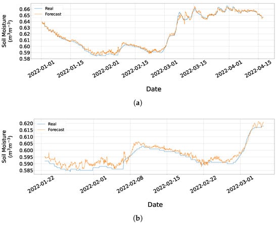
Figure 9.
Forecast of 48 h of for the evaluation dataset consisting of 7-day hourly data of P, T, , , , and . (a) Forecast for the evaluation dataset. (b) Zoom of subfigure (a) from 22 January 2022 to 4 March 2022.
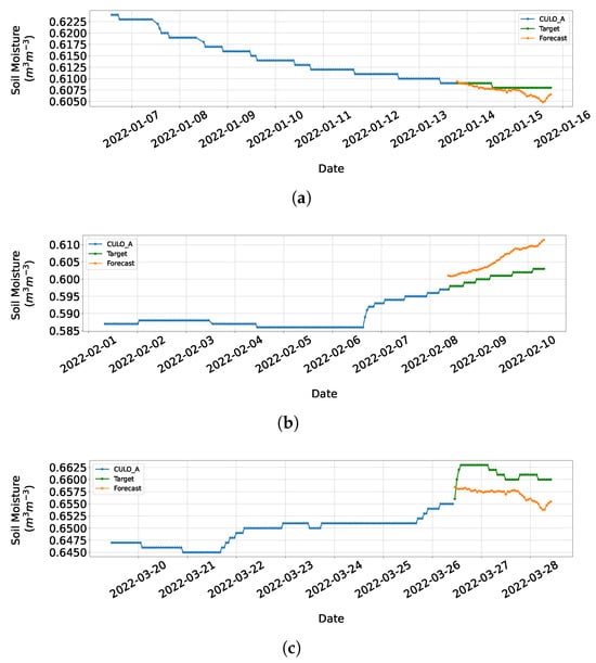
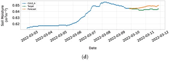
Figure 10.
Forecast for different time points of the evaluation series . (a) Forecast of the evaluation series as of 14 January 2022. (b) Forecast of the evaluation series as of 8 February 2022. (c) Forecast of the evaluation series as of 26 March 2022. (d). Forecast of the evaluation series as of 9 March 2022.
The evaluated base network was capable of predicting for the next 48 h, using the environmental variables P, T, , , , and from the previous seven days. Regarding the performance evaluation metrics, as shown in Table 7, the loss function used during the network training achieved a minimum value of in the training set. In terms of prediction accuracy, the base network showed a mean absolute error (MAE) of 0.0025, a root mean squared error (RMSE) of 0.0036, and a mean squared logarithmic error (MSLE) of in the training set. Overall, these results indicate that the evaluated base network performed well in the training set but not as well in the validation and evaluation sets, suggesting a slight degree of overfitting to the training data. Additionally, it was found that the network’s ability to fit to the actual values varied depending on the metric used and the evaluated dataset.

Table 7.
Metric results obtained for the base network predicting 48 h of , given P, T, , , , and data from seven days.
4.2.3. Application of the Base Network for Soil Moisture Forecasting under Tussock Grass Using Transfer Learning
In this section, the results of applying transfer-learning techniques in similar domains are presented, including forecasts and the evaluation of the results with the established metrics in the methodology. Based on the knowledge acquired from the base network and through use of transfer-learning techniques, 48 h soil moisture forecasts were made for , , , , , , , , and Figure 11a–h. The models used hourly information from the previous 7 days as input, using the same domain as the base network: P, T, , , , and .

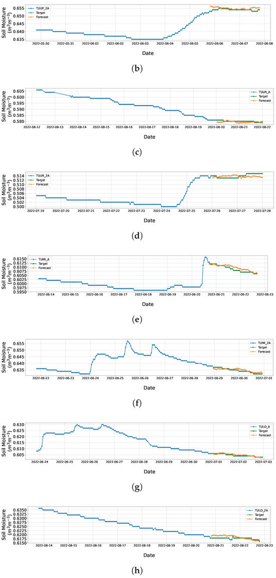
Figure 11.
Forecasts of soil moisture under tussock grasses for different topographic positions and soil horizons. (a) Forecast of using transfer learning from base network . (b) Forecast of using transfer learning from base network . (c) Forecast of using transfer learning from base network . (d) Forecast of using transfer learning from base network . (e) Forecast of using transfer learning from base network . (f) Forecast of using transfer learning from base network . (g) Forecast of using transfer learning from base network . (h) Forecast of using transfer learning from base network .
Table 8 shows the performance metrics for deep networks forecasting 48 h using the variables P, T, , , , and . The metrics include statistics such as loss, MAE, RMSE, and MSLE for the training, validation, and evaluation datasets. Remarkably promising results are observed in this table. The bold-highlighted values indicate particularly outstanding performance. For instance, a loss of for in the training set denotes an excellent model capacity to fit the training data.

Table 8.
Metrics obtained for deep networks forecasting 48 h of using information from the variables: P, T, , , , and .
MAE and RMSE are also notable, with values as low as and , respectively. These numbers suggest that the models have outstanding accuracy in predicting under diverse conditions. The MSLE, with values on the scale of , indicates that the models are particularly effective in predicting within a logarithmic environment, crucial in many applications.
4.2.4. Application of the Base Network for Soil Moisture Forecasting under Cushion-Forming Plants Using Transfer-Learning
In this section, we present the results of the application of the transfer-learning techniques in similar domains, presenting the forecasts and evaluation of the results for cushion plants with the metrics established in the methodology. Figure 12 shows the forecast of 48 h of soil moisture for all the profiles and horizons of cushion plants, where we used 7 days of hourly information as input, with the same domain as the base network: P, T, , , , and . Figure 12a–g show forecasts for different moments of the evaluation series: , , , , , , , and .
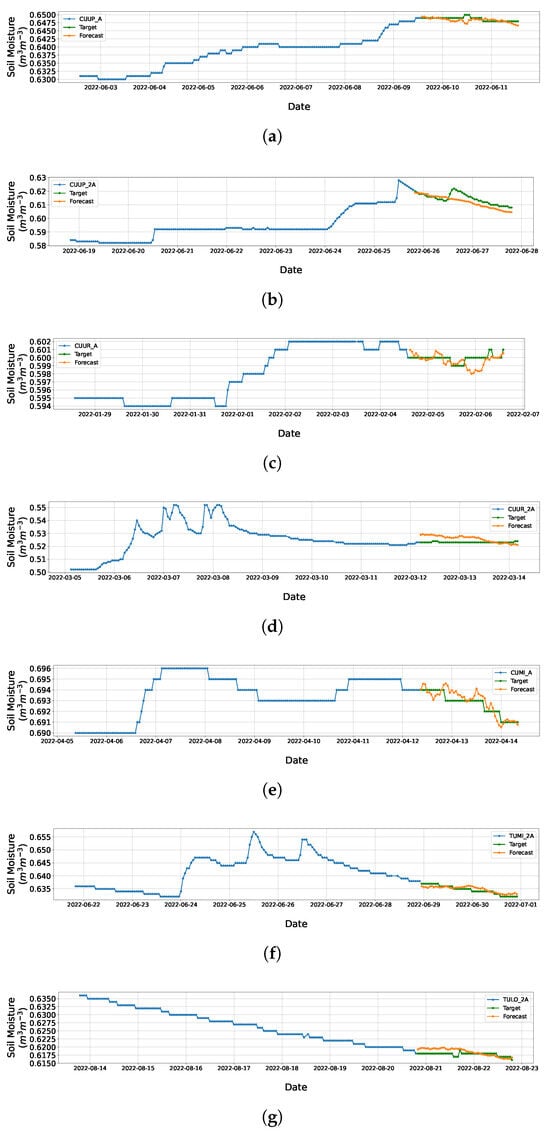
Figure 12.
Forecasts at different moments of soil moisture in tussock grass across all profiles and horizons analyzed. (a) Forecast of using transfer learning from the base network . (b) Forecast of using transfer learning from the base network . (c) Forecast of using transfer learning from the base network . (d) Forecast of using transfer learning from the base network . (e) Forecast of using transfer learning from the base network . (f) Forecast of using transfer learning from the base network . (g) Forecast of using transfer learning from the base network .
Table 9 presents the performance metrics for the deep learning models. A notable feature of this table is the values highlighted in bold. For instance, in the case of in the training set, an extraordinarily low loss of is observed, reflecting the exceptional capacity of the model to fit the training data. This level of precision is reinforced by an MAE and RMSE of and , respectively, indicating outstanding performance in predicting . The MSLE values are also noteworthy, with figures in the order of , suggesting that the models are highly effective in predicting in a logarithmic environment. Overall, the performance metrics illustrate the potential of deep learning models in predicting , demonstrating exceptional accuracy across various datasets. These results support the potential utility of these models in practical applications requiring precise forecasts based on multiple inputs.

Table 9.
Metrics obtained for deep learning models predicting 48 h of using information from variables P, T, , , , and .
5. Discussion
The present study has demonstrated the effectiveness of utilizing neural networks and transfer-learning techniques in soil-moisture forecasting in the high-elevation Ecuadorian Andes. However, numerous opportunities exist to expand and apply these findings in different areas of interest.
One potential avenue for future research is the application of the developed models in landslide or mass movement prediction. Soil moisture plays a crucial role in slope and hillside stability, and its accurate prediction could provide a valuable tool for landslide forecasting using, e.g., hydrometeorological threshold approaches. Integrating precipitation, temperature, and soil moisture data into landslide prediction models could help identify critical thresholds and generate early warnings to mitigate risks associated with these events.
Another area of potential application is wildfire forecasting. Precise soil moisture information can aid in assessing the level of wildfire risk. By combining soil moisture data with relevant climatic variables, such as precipitation, temperature, relative humidity, and solar radiation, predictive models could be developed to identify favorable conditions for fire propagation. These forecasts could contribute to risk management planning and decision-making, enabling a more effective and timely response.
Furthermore, the results of this research offer the possibility of using them as input to estimate the amount of available water in a watershed. Soil moisture is a key indicator of water availability for vegetation and overall water resources. By combining soil moisture data obtained through forecasting models with additional information about the hydrological characteristics of a watershed, reliable estimates of stored water quantity and its availability for various purposes, such as agriculture, drinking water supply, and hydroelectric power generation, could be developed.
These possibilities are only a few of the potential applications that arise from the results obtained in this study. Exploring and expanding these applications, as well as considering other areas where accurate soil moisture forecasting could have a significant impact, represent promising avenues for future research. Developing more complex models, optimizing the number of variables that best contribute to soil moisture forecasting, and refining transfer-learning techniques are exciting challenges for future investigations in this field.
Our study faces significant limitations concerning the generalizability of the results, as transfer learning can be challenging when there are environmental differences between training and prediction areas. The limited availability of locations with similar measurement capabilities can also affect the generalization of our methodology. Additionally, the analysis was based on a period of nearly four years of data, which may not fully capture soil moisture variability; this could bias our results towards the specific conditions of the northern Ecuadorian páramo and fail to reflect natural variability over time. Therefore, it is important to interpret our findings with caution.
In the research conducted by Páez-Bimos et al. [33], where the dynamic model HYDRUS-1D was employed, a precision in soil moisture forecasts was achieved, with values ranging from 0.49 to 0.91 and RMSE ≤ 0.02 cm3 cm−3. In contrast, our implementation of neural networks showed minimal losses of and a minimum RMSE of 0.0036, with high efficiency coefficients such as an NSE and KGE of 0.97. Both approaches provide effective representations of hydrological processes, with specific strengths in accuracy and applicability.
6. Conclusions
State-of-the-art models employing neural networks, specifically CNN–LSTM–ANN, were utilized to forecast 48 h soil moisture at various depths and locations using seven days of hourly information. The neural network employed in this study is a deep architecture with optimized hyperparameters, enabling the neurons to effectively capture the relationship between hydrometeorological variables and soil moisture. The forecast evaluation metrics indicate promising results, with an error range of .
The employed transfer-learning technique with network-based transfer learning served a dual purpose: firstly, it demonstrated the ability to transfer knowledge from one specific domain, i.e., a soil profile, to another related domain, i.e., a different soil profile located in a different site; secondly, it indirectly optimized the training time of the neural networks that utilized the pre-trained base network.
Author Contributions
Conceptualization, V.V., M.V., D.E.-G. and S.P.-B.; experimental design, V.V. and S.P.-B.; data collection, S.P.-B. and M.V.; data validation, S.P.-B. and D.E.-G.; funding acquisition, V.V. and M.V.; project administration, V.V. and M.V.; writing—original draft, D.E.-G.; writing—review and editing, all the authors. All authors have read and agreed to the published version of the manuscript.
Funding
This research has been supported by the Académie de Recherche et Enseignement Supérieur de la Fédération Wallonie-Bruxelles (ARES CCD) through the PDR project páramoSUS (2017–2023) and was realized in collaboration with the Fondo para la Protección del Agua (FONAG), the Empresa Pública Metropolitana de Agua Potable y Saneamiento (EPMAPS), the Programa para el Manejo de Agua y Suelo (PROMAS) of the Facultad de Ingeniería Civil of the Universidad de Cuenca, the Empresa Pública Municipal de Telecomunicaciones, Agua Potable, Alcantarillado y Saneamiento de Cuenca (ETAPA-EP), and ElecAustro.
Data Availability Statement
Data will be made available by the authors upon reasonable request.
Acknowledgments
We thank Jordan Cruz, Isaías Quinatoa, and undergraduate students from the Escuela Politécnica Nacional (EPN) and Universidad Central del Ecuador (UCE) for their help in the preparation and sampling of the field campaigns in Antisana. This research has been supported by the research cooperation project “Linking Global Change with Soil and Water Conservation in the High Andes” (páramoSus). SPB was supported by EPN in the development of his doctoral program, and DEG would like to thank Viviana Velasteguí for her support in GIS. Additionally, DEG received continuous support from EPMAPS during his MSc program.
Conflicts of Interest
The authors declare no conflicts of interest.
References
- Oki, T.; Kanae, S. Global hydrological cycles and world water resources. Science 2006, 313, 1068–1072. [Google Scholar] [CrossRef] [PubMed]
- Trenberth, K.E.; Fasullo, J.T.; Kiehl, J. Earth’s global energy budget. Bull. Am. Meteorol. Soc. 2009, 90, 311–324. [Google Scholar] [CrossRef]
- Berg, A.; Sheffield, J. Climate Change and Drought: The Soil Moisture Perspective. Curr. Clim. Chang. Rep. 2018, 4, 180–191. [Google Scholar] [CrossRef]
- Seneviratne, S.I.; Corti, T.; Davin, E.L.; Hirschi, M.; Jaeger, E.B.; Lehner, I.; Orlowsky, B.; Teuling, A.J. Investigating soil moisture—Climate interactions in a changing climate: A review. Earth-Sci. Rev. 2010, 99, 125–161. [Google Scholar] [CrossRef]
- Mukhlisin, M.; Astuti, H.W.; Wardihani, E.D.; Matlan, S.J. Techniques for ground-based soil moisture measurement: A detailed overview. Arab. J. Geosci. 2021, 14, 2032. [Google Scholar] [CrossRef]
- Kelly, E.F.; Chadwick, O.A.; Hilinski, T.E. The effect of plants on mineral weathering. Biogeochemistry 1998, 42, 21–53. [Google Scholar] [CrossRef]
- Páez-Bimos, S.; Molina, A.; Calispa, M.; Delmelle, P.; Lahuatte, B.; Villacís, M.; Muñoz, T.; Vanacker, V. Soil-vegetation-water interactions controlling solute flow and chemical weathering in volcanic ash soils of the high Andes. Hydrol. Earth Syst. Sci. 2023, 27, 1507–1529. [Google Scholar] [CrossRef]
- Brück, S.A.; Torres, B.D.M.; de Lourdes Teixeira de Moraes Polizeli, M. The Ecuadorian páramo in danger: What we know and what might be learned from northern wetlands. Glob. Ecol. Conserv. 2023, 47, e02639. [Google Scholar] [CrossRef]
- Patiño, D.T.; Sánchez, P.C.; Rojas, G.M. Umbrales en la respuesta de humedad del suelo a condiciones meteorológicas en una ladera Altoandina. Maskana 2018, 9, 53–65. [Google Scholar] [CrossRef]
- Vanacker, V.; Molina, A.; Torres, R.; Calderon, E.; Cadilhac, L. Challenges for research on global change in mainland Ecuador. Neotrop. Biodivers. 2018, 4, 114–118. [Google Scholar] [CrossRef]
- Tenorio, G.E.; Vanacker, V.; Campforts, B.; Álvarez, L.; Zhiminaicela, S.; Vercruysse, K.; Molina, A.; Govers, G. Tracking spatial variation in river load from Andean highlands to inter-Andean valleys. Geomorphology 2018, 308, 175–189. [Google Scholar] [CrossRef]
- Ruiz-Hernández, J.C.; Condom, T.; Ribstein, P.; Le Moine, N.; Espinoza, J.C.; Junquas, C.; Villacís, M.; Vera, A.; Muñoz, T.; Maisincho, L.; et al. Spatial variability of diurnal to seasonal cycles of precipitation from a high-altitude equatorial Andean valley to the Amazon Basin. J. Hydrol. Reg. Stud. 2021, 38, 100924. [Google Scholar] [CrossRef]
- Molina, A.; Vanacker, V.; Corre, M.D.; Veldkamp, E. Patterns in Soil Chemical Weathering Related to Topographic Gradients and Vegetation Structure in a High Andean Tropical Ecosystem. J. Geophys. Res. Earth Surf. 2019, 124, 666–685. [Google Scholar] [CrossRef]
- Buytaert, W.; Cuesta-Camacho, F.; Tobón, C. Potential impacts of climate change on the environmental services of humid tropical alpine regions. Glob. Ecol. Biogeogr. 2011, 20, 19–33. [Google Scholar] [CrossRef]
- Buytaert, W.; Célleri, R.; De Bièvre, B.; Cisneros, F.; Wyseure, G.; Deckers, J.; Hofstede, R. Human impact on the hydrology of the Andean páramos. Earth-Sci. Rev. 2006, 79, 53–72. [Google Scholar] [CrossRef]
- Bonnesoeur, V.; Locatelli, B.; Guariguata, M.R.; Ochoa-Tocachi, B.F.; Vanacker, V.; Mao, Z.; Stokes, A.; Mathez-Stiefel, S.L. Impacts of forests and forestation on hydrological services in the Andes: A systematic review. For. Ecol. Manag. 2019, 433, 569–584. [Google Scholar] [CrossRef]
- Iñiguez, V.; Morales, O.; Cisneros, F.; Bauwens, W.; Wyseure, G. Analysis of the drought recovery of Andosols on southern Ecuadorian Andean páramos. Hydrol. Earth Syst. Sci. 2016, 20, 2421–2435. [Google Scholar] [CrossRef]
- Gonzalez-Zeas, D.; Erazo, B.; Lloret, P.; Steinschneider, S.; Dangles, O. Linking global climate change to local water availability: Limitations and prospects for a tropical mountain watershed. J. Sci. Tot. Env. 2019, 650, 2577–2586. [Google Scholar] [CrossRef]
- Molina, A.; Govers, G.; Vanacker, V.; Poesen, J.; Zeelmaekers, E.; Cisneros, F. Runoff generation in a degraded Andean ecosystem: Interaction of vegetation cover and land use. Catena 2007, 71, 357–370. [Google Scholar] [CrossRef]
- Molina, A.; Govers, G.; Cisneros, F.; Vanacker, V. Vegetation and topographic controls on sediment deposition and storage on gully beds in a degraded mountain area. Earth Surf. Processes Landforms 2009, 34, 755–767. [Google Scholar] [CrossRef]
- Mosquera, G.M.; Crespo, P.; Breuer, L.; Feyen, J.; Windhorst, D. Water transport and tracer mixing in volcanic ash soils at a tropical hillslope: A wet layered sloping sponge. Hydrol. Processes 2020, 34, 2032–2047. [Google Scholar] [CrossRef]
- Prasad, R.; Deo, R.C.; Li, Y.; Maraseni, T. Weekly soil moisture forecasting with multivariate sequential, ensemble empirical mode decomposition and Boruta-random forest hybridizer algorithm approach. Catena 2019, 177, 149–166. [Google Scholar] [CrossRef]
- Gao, P.; Qiu, H.; Lan, Y.; Wang, W.; Chen, W.; Han, X.; Lu, J. Modeling for the Prediction of Soil Moisture in Litchi Orchard with Deep Long Short-Term Memory. Agriculture 2021, 12, 25. [Google Scholar] [CrossRef]
- Han, H.; Choi, C.; Kim, J.; Morrison, R.R.; Jung, J.; Kim, H.S. Multiple-depth soil moisture estimates using artificial neural network and long short-term memory models. Water 2021, 13, 2584. [Google Scholar] [CrossRef]
- Suebsombut, P.; Sekhari, A.; Sureephong, P.; Belhi, A.; Bouras, A. Field data forecasting using LSTM and Bi-LSTM approaches. Appl. Sci. 2021, 11, 11820. [Google Scholar] [CrossRef]
- Sivasankaran, S.; Mohan, K.J.; Nazer, G.M. Soil Moisture Quantity Prediction using Optimized Deep Learning Supported model for Sustainable cultivation of Groundnut plant. Nat. Volatiles Essent. Oils J. NVEO 2021, 8, 13184–13205. [Google Scholar]
- Liu, D.; Liu, C.; Tang, Y.; Gong, C. A GA-BP Neural Network Regression Model for Predicting Soil Moisture in Slope Ecological Protection. Sustainability 2022, 14, 1386. [Google Scholar] [CrossRef]
- Zhang, L.; Xue, Z.; Zhang, Y.; Ma, J.; Li, H. Enhanced Generalized Regression Neural Network for Soil Moisture Estimation Over the Qinghai-Tibet Plateau. IEEE J. Sel. Top. Appl. Earth Obs. Remote Sens. 2022, 15, 3815–3829. [Google Scholar] [CrossRef]
- Prasad, R.; Deo, R.C.; Li, Y.; Maraseni, T. Soil moisture forecasting by a hybrid machine learning technique: ELM integrated with ensemble empirical mode decomposition. Geoderma 2018, 330, 136–161. [Google Scholar] [CrossRef]
- Rostami, S.; He, J.; Hassan, Q.K. Riverine water quality response to precipitation and its change. Environments 2018, 5, 8. [Google Scholar] [CrossRef]
- Vanacker, V.; Vanderschaeghe, M.; Govers, G.; Willems, E.; Poesen, J.; Deckers, J.; De Bievre, B. Linking hydrological, infinite slope stability and land-use change models through GIS for assessing the impact of deforestation on slope stability in high Andean watersheds. Geomorphology 2003, 52, 299–315. [Google Scholar] [CrossRef]
- Zhao, B.; Dai, Q.; Zhuo, L.; Zhu, S.; Shen, Q.; Han, D. Assessing the potential of different satellite soil moisture products in landslide hazard assessment. Remote Sens. Environ. 2021, 264, 112583. [Google Scholar] [CrossRef]
- Páez-Bimos, S.; Villacís, M.; Morales, O.; Calispa, M.; Molina, A.; Salgado, S.; de Bievre, B.; Delmelle, P.; Muñoz, T.; Vanacker, V. Vegetation effects on soil pore structure and hydraulic properties in volcanic ash soils of the high Andes. Hydrol. Processes 2022, 36, e14678. [Google Scholar] [CrossRef]
- Lahuatte, B.; Mosquera, G.M.; Páez-Bimos, S.; Calispa, M.; Vanacker, V.; Zapata-Ríos, X.; Muñoz, T.; Crespo, P. Delineation of water flow paths in a tropical Andean headwater catchment with deep soils and permeable bedrock. Hydrol. Processes 2022, 36, e14725. [Google Scholar] [CrossRef]
- Empresa Pública Metropolitana de Agua Potable y Saneamiento (EPMAPS) y Fideicomiso Mercantil Fondo Ambiental para la Protección de las Cuencas y Agua (FONAG). Actualización del Plan de Manejo del Área de Conservación Hídrica Antisana; EPMAPS-FONAG: Quito, Ecuador, 2018. [Google Scholar]
- Fideicomiso Mercantil Fondo Ambiental para la Protección de las Cuencas y Agua (FONAG). Plan estrategico 2021-2025; FONAG: Quito, Ecuador, 2020. [Google Scholar]
- Espinosa, J.; Moreno, J.; Bernal, G. The Soils of Ecuador; World Soils Book Series; Springer International: Cham, Switzerland, 2017. [Google Scholar]
- Hall, M.L.; Mothes, P.A.; Samaniego, P.; Militzer, A.; Beate, B.; Ramón, P.; Robin, C. Antisana volcano: A representative andesitic volcano of the eastern cordillera of Ecuador: Petrography, chemistry, tephra and glacial stratigraphy. J. South Am. Earth Sci. 2017, 73, 50–64. [Google Scholar] [CrossRef]
- Zhuang, F.; Qi, Z.; Duan, K.; Xi, D.; Zhu, Y.; Zhu, H.; Xiong, H.; He, Q. A comprehensive survey on transfer learning. Proc. IEEE 2020, 109, 43–76. [Google Scholar] [CrossRef]
- Alpaydin, E. Machine Learning: The New AI; MIT Press: Cambridge, MA, USA, 2016. [Google Scholar]
- Kelleher, J.D.; Tierney, B.; Tierney, B. Data Science; MIT Press: Cambridge, MA, USA, 2018. [Google Scholar]
- Goodfellow, I.; Bengio, Y.; Courville, A. Deep Learning; MIT Press: Cambridge, MA, USA, 2016. [Google Scholar]
- Sit, M.; Demiray, B.Z.; Xiang, Z.; Ewing, G.J.; Sermet, Y.; Demir, I. A comprehensive review of deep learning applications in hydrology and water resources. Water Sci. Technol. 2020, 82, 2635–2670. [Google Scholar] [CrossRef]
- Tan, C.; Sun, F.; Kong, T.; Zhang, W.; Yang, C.; Liu, C. A survey on deep transfer learning. In Proceedings of the International Conference on Artificial Neural Networks, Rhodes, Greece, 4–7 October 2018; Springer: Cham, Switzerland, 2018; pp. 270–279. [Google Scholar]
Disclaimer/Publisher’s Note: The statements, opinions and data contained in all publications are solely those of the individual author(s) and contributor(s) and not of MDPI and/or the editor(s). MDPI and/or the editor(s) disclaim responsibility for any injury to people or property resulting from any ideas, methods, instructions or products referred to in the content. |
© 2024 by the authors. Licensee MDPI, Basel, Switzerland. This article is an open access article distributed under the terms and conditions of the Creative Commons Attribution (CC BY) license (https://creativecommons.org/licenses/by/4.0/).