Urban Water Demand Prediction Based on Attention Mechanism Graph Convolutional Network-Long Short-Term Memory

Abstract

Predicting short-term urban water demand is essential for water resource management and directly impacts urban water resource planning and supply–demand balance. As numerous factors impact the prediction of short-term urban water demand and present complex nonlinear dynamic characteristics, the current water demand prediction methods mainly focus on the time dimension characteristics of the variables, while ignoring the potential influence of spatial characteristics on the temporal characteristics of the variables. This leads to low prediction accuracy. To address this problem, a short-term urban water demand prediction model which integrates both spatial and temporal characteristics is proposed in this paper. Firstly, anomaly detection and correction are conducted using the Prophet model. Secondly, the maximum information coefficient (MIC) is used to construct an adjacency matrix among variables, which is combined with a graph convolutional neural network (GCN) to extract spatial characteristics among variables, while a multi-head attention mechanism is applied to enhance key features related to water use data, reducing the influence of unnecessary factors. Finally, the prediction of short-term urban water demand is made through a three-layer long short-term memory (LSTM) network. Compared with existing prediction models, the hybrid model proposed in this study reduces the average absolute percentage error by 1.868–2.718%, showing better prediction accuracy and prediction effectiveness. This study can assist cities in rationally allocating water resources and lay a foundation for future research.

1. Introduction

Despite China’s abundant total freshwater resources, the freshwater available per capita remains relatively low [1]. Accelerated urbanization has led most Chinese cities to face the challenges of water scarcity, making the rational planning of urban residential water use crucial in resolving the supply–demand conundrum of water resources [2]. Urban residential water consumption, influenced by a myriad of factors, exhibits complex nonlinear dynamic characteristics [3,4]. Traditional methods based on human experience are inadequate for predicting intricate water usage trends, whereas urban water demand prediction can effectively reveal consumption trends and inform the effective distribution and usage of water resources. Urban water demand prediction is categorized into short-term, medium-term, and long-term prediction [5], with short-term prediction being particularly crucial for water resource management due to its immediacy and urgency. Through accurate short-term water demand prediction, cities can adjust their water supply strategies over time, effectively reduce energy consumption and costs, and improve the overall efficiency of the water supply system [6,7,8].

Current short-term water demand prediction methods include traditional back propagation (BP) neural networks [9,10,11], grey models [12,13], support vector machines (SVMs) [14,15], random forests [16], and regression analysis models [17,18]. While effective under certain conditions, these methods generally face limitations in their generalization ability and predictive accuracy. With the advances in deep learning and neural network technologies, these methods have been extensively applied to urban water demand prediction. Particularly, the long short-term memory (LSTM) model [19,20] has demonstrated exceptional performance in water demand forecasting, adeptly handling data with high temporal resolution, abrupt changes, and uncertainties, as well as incorporating additional information such as the day of the week or national holidays. Nonetheless, the impacts of climatic conditions and data noise on prediction accuracy remain significant challenges. To address this, Du et al. [7] developed a model capable of managing complex data patterns and capturing peaks in time series, employing discrete wavelet transform (DWT) and principal component analysis (PCA) to generate variance-stabilized, low-dimensional, high-quality input variables. Al-Ghamdi et al. [21] utilized artificial neural networks (ANNs) to predict daily water demand under climatic conditions, adjusting the ANN hyperparameters with particle swarm optimization (PSO), and identified the dew point as the climatic condition with the most significant impact on water demand. Zubaidi et al. [22] employed a combination of data preprocessing and an ANN optimized with the backtracking search algorithm (BSA-ANN) to estimate monthly water demand related to previous usage, proving the model’s capability for high-accuracy water demand forecasting in cities severely affected by climate change and population growth. These models have enhanced the ability to process complex data by integrating various techniques, yet have not fully considered non-stationarity and nonlinearity under multi-variable influences. To overcome this issue, Li et al. [23] proposed a composite prediction model for urban water usage based on the new information priority theory (CPMBNIP), which more effectively utilizes new data to improve predictions for certain non-stationary time series. Hu et al. [24] and Zhou et al. [4] employed a hybrid model combining convolutional neural networks and bidirectional long short-term memory networks, considering the correlations among multiple variables to predict water demand under a range of nonlinear and uncertain temporal patterns.

Despite significant advancements, the current approaches predominantly rely on extracting the temporal features of time series data, overlooking the influence of spatial characteristics on these temporal characteristics. Current studies on spatiotemporal features primarily focus on multi-site analysis. For instance, Zheng et al. [25] predicted daily variations in water quality parameters across 138 watersheds in southern China using variables such as meteorology, land use, and socioeconomic factors, employing the SHapley Additive exPlanations method to identify significant variables and infer the direction of their impact on water quality changes, effectively explaining the prediction results. Wang et al. [26] identified complex relationships between various meteorological factors at different sites and dissolved oxygen (DO) concentration levels, demonstrating that the integration of graph-based learning and time transformers in environmental modeling is a promising direction for future research. Zanfei et al. [27] developed a novel graph convolutional recurrent neural network (GCRNN) to analyze the spatial and temporal dependencies among different water-demand time series within the same geographical area. Wang et al. [28] presented an LSTM model integrating spatiotemporal attention, focusing on more valuable time and spatial features, to predict water levels in the middle and lower reaches of the Han River. However, these studies have focused on correlations between spatial features at multiple observation sites rather than between the spatial features of different variables, which also affect the temporal features of the water use data, an aspect that has not been adequately considered in previous studies.

Based on this background, this paper combines the spatial and temporal features of variables and proposes an attention mechanism graph convolutional neural network–long short-term memory model (GCN-Att-LSTM). Compared with other approaches, this method exhibits a similar level of complexity, and yet it excels in achieving more precise short-term urban water demand predictions. Initially, the principles of the Prophet model are utilized for anomaly detection and correction in water data to enhance data quality. Subsequently, the maximal information coefficient (MIC) calculates the correlation between meteorological and water usage data. Building on this, the graph convolutional network (GCN) extracts spatial features between water consumption and meteorological data, with a multi-head attention mechanism applied to weigh these spatial features. Finally, the processed data are input into a three-layer LSTM with residual connections added to improve water demand prediction accuracy.

The structure of this paper is as follows: Section 2 details the sources and data processing of urban water data. Section 3 introduces the methods employed in the GCN-Att-LSTM model. Section 4 analyzes the experimental results to verify the model’s performance. Finally, Section 5 concludes and presents the research findings.

2. Materials

2.1. Data Source

This study selected Beijing, located in the northern part of China on the east side of the Yellow River, as the research subject. Beijing is situated between longitudes 115°25′ E and 117°30′ E, and latitudes 39°28′ N and 41°05′ N. It is characterized by a temperate semi-humid continental climate with distinct seasons and relatively low precipitation. In such a climatic context, the rational allocation of water resources is of vital significance for socio-economic and sustainable urban development.

The data employed in this study consist of daily water usage records provided by the Beijing Water Authority from 1 September 2016 to 1 August 2023. Of these data, 80% are allocated for training, while the remaining 20% are reserved for testing. The date for the training and test set splits is 13 March 2022. Additionally, the meteorological data for Beijing from the National Meteorological Information Center are incorporated, covering 15 meteorological elements, including maximum temperature (f₀), minimum temperature (f₁), average temperature (f₂), maximum dew point (f₃), minimum dew point (f₄), average dew point (f₅), average rainfall (f₆), maximum humidity (f₇), minimum humidity (f₈), average humidity (f₉), average sea-level atmospheric pressure (f₁₀), average meteorological station atmospheric pressure (f₁₁), average horizontal visibility (f₁₂), average wind speed (f₁₃), and maximum rainfall (f₁₄), as shown in

Table 1. Influencing factors of urban water demand.

Category	Physical Meaning	Parameter
Temperature	Maximum Temperature (°C)	f0
	Minimum Temperature (°C)	f1
	Average Temperature (°C)	f2
Dew Point	Maximum Dew Point (°C)	f3
	Minimum Dew Point (°C)	f4
	Average Dew Point (°C)	f5
Rainfall	Average Rainfall (mm)	f6
	Maximum Rainfall (mm)	f14
Humidity	Maximum Humidity (%)	f7
	Minimum Humidity (%)	f8
	Average Humidity (%)	f9
Atmospheric Pressure	Average Sea-Level Atmospheric Pressure (mmHg)	f10
	Average Meteorological Station Atmospheric Pressure (mmHg)	f11
Visibility	Average Horizontal Visibility (km)	f12
Wind Speed	Average Wind Speed (m·s−1)	f13

.

2.2. Data Analysis

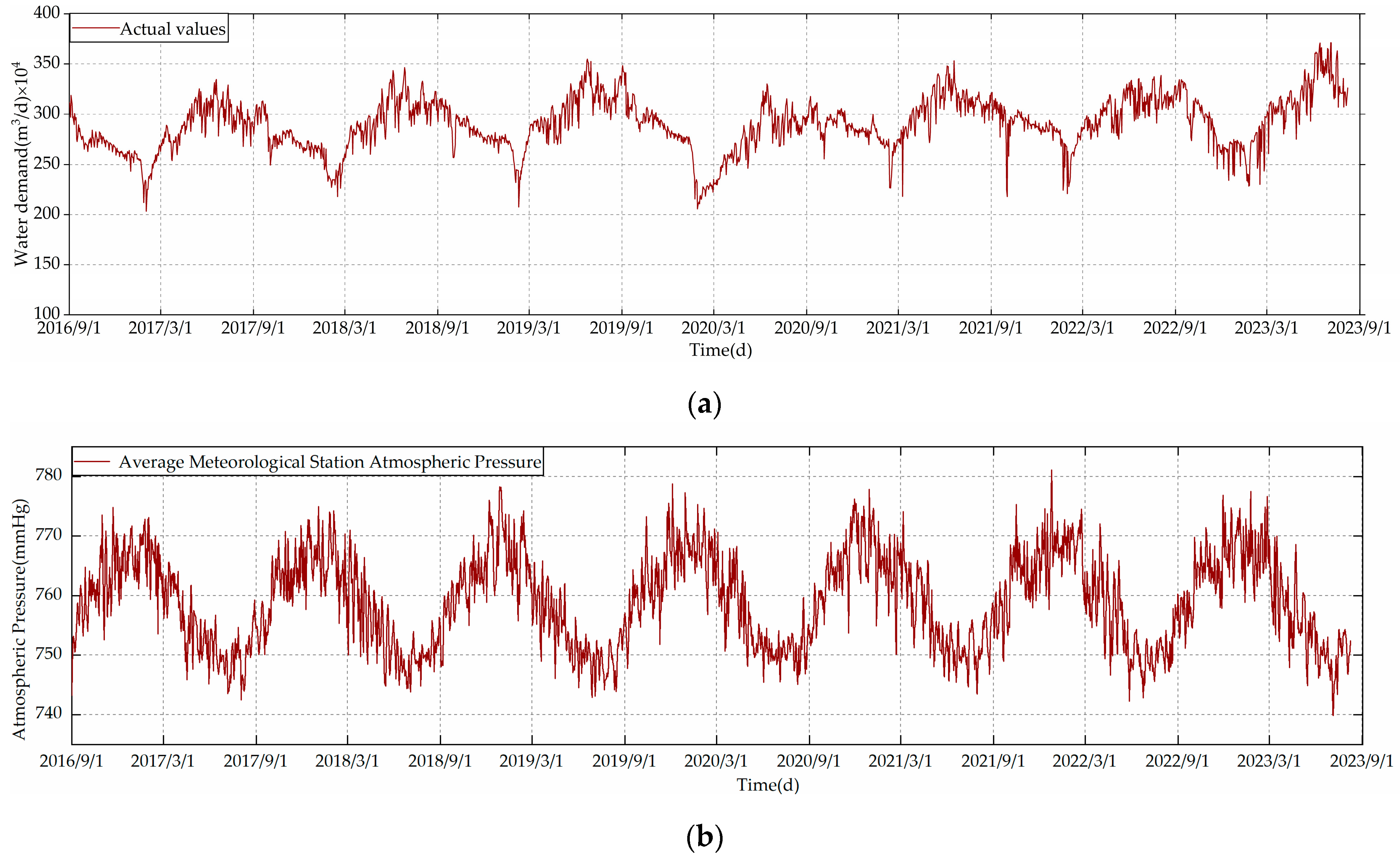
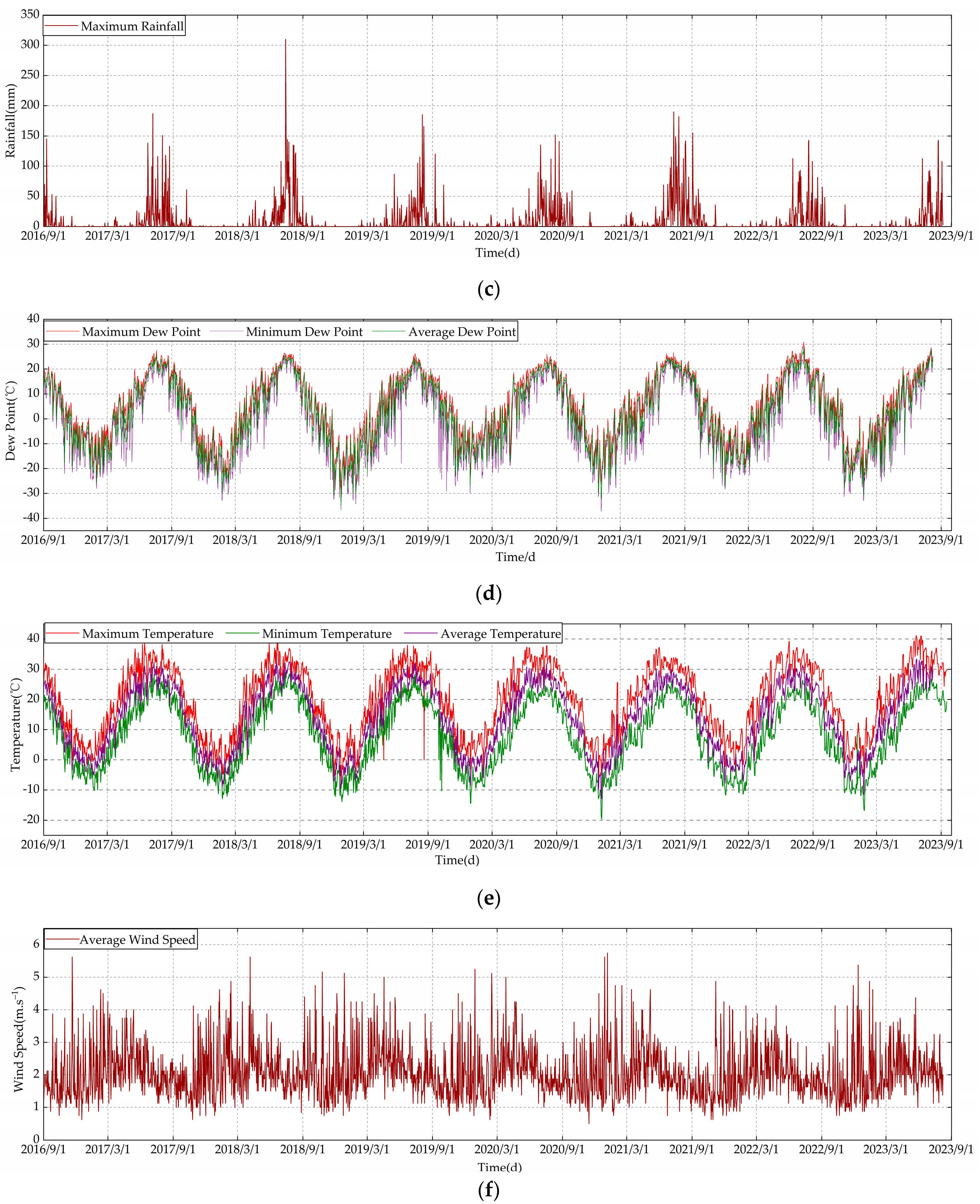
To explore the dynamic fluctuations in residential urban water demand, this study meticulously selected water demand and closely associated climatic factors, including variables f₀ through f₅, f₁₁, f₁₃, and f₁₄. The criteria for the selection of these variables are detailed in Section 4.3. Following the selection process, visualizations for each variable were conducted, as depicted in Figure 1. Among these, the highest temperature reaches 41 °C, with the maximum daily water demand at 3.758 million cubic meters. The lowest temperature is −19 °C, with the minimum daily water demand at 2.034 million cubic meters. The annual average precipitation is only 577 mm. The graph also indicates that these variables exhibit certain trends of change. To quantitatively assess the trend changes in urban water demand (y) relative to various meteorological factors, the Mann–Kendall trend test was employed. This method is used to evaluate trend changes in time series data, where a positive Z-value indicates an upward trend, and a negative Z-value signifies a downward trend. Trends were deemed statistically significant at the 95% confidence level when p-values were less than 0.05. The outcomes of this analysis are succinctly presented in

Table 2. Trend analysis of climate factors and water use data.

Category	p	Z
f0	1.7119 × 10−12	7.0561
f1	0.9435	0.0708
f2	0.0077	2.6608
f3	0.0023	3.0373
f4	0.0224	2.2831
f5	0.0088	2.6160
f11	0.83264	0.2113
f13	0.0727	−1.7941
f14	7.9589 × 10−12	−6.8392
y	0.0	14.0557

, revealing significant trend changes for variables f₀, f₂, f₃, f₄, f₅, f₁₄, and y. Conversely, the trends for variables f₁, f₁₁, and f₁₃ did not reach statistical significance, which may be related to the quality of the data, the size of the sample, and the range of the data.

To further dissect the seasonality of water resources on an annual basis (according to the solar calendar, spring is March–May, summer is June–August, autumn is September–November, and winter is December–February), this investigation selected data segments from 2017 to 2022 for analysis, encompassing complete yearly records. Figure 2 illustrates the annual water usage data for this period, highlighting a pattern of comparatively lower water consumption during the winter and spring months, followed by a notable increase during the summer. To elucidate the annual trends in water consumption with greater clarity, the Mann–Kendall trend test was applied to the water usage data spanning from 2017 to 2022. As summarized in

Table 3. Trend analysis of water use data, 2017–2022.

Year	p	Z
2017	0.0	9.2061
2018	1.9539 × 10−5	4.2700
2019	1.4035 × 10−6	4.8244
2020	0.0	11.8820
2021	0.0003	3.0412
2022	0.0002	3.6244

, the analysis revealed that the p-values for each year were below 0.05, affirming the presence of significant trend variations in the annual water consumption data.

2.3. Data Processing

In response to the characteristics of seasonality, cyclicity, and holidays within the chronological dataset of Beijing’s water usage, this study employs the Prophet model for anomaly detection and correction. The Prophet [29] model is an efficient prediction tool specifically designed for time series data with pronounced seasonal and holiday effects. The core of the model resides in decomposing the time series into four main components: trend, seasonality, holidays, and residual, to deeply analyze and simulate the inherent patterns of the data. Specifically, the time series decomposition formula is as follows:

$$y(t)=g(t)+s(t)+h(t)+\epsilon (t)$$

(1)

where t signifies the time; $y(t)$ is the daily urban water demand chronology; $g(t)$ represents the trend aspect, indicating the non-cyclical trend of the chronology. It is usually set as a piecewise linear or logistic growth curve to capture the overall direction of the time series data over time; $s(t)$ is the seasonal aspect, reflecting the impact with a fixed cyclicity. Prophet fits seasonal effects with Fourier series to model the cyclical nature of these patterns; $h(t)$ is the holiday component, denoting the influence on the time series on specific dates. Prophet allows users to explicitly include these events by providing a custom list of holidays. The model then estimates the effect of these holidays on the time series data; $\epsilon (t)$ is the error term, representing fluctuations not predicted by the model. It is assumed to be normally distributed, capturing random variations in the time series data that the model’s components (trend, seasonality, and holidays) do not explain.

The Prophet model predicts each component of the time series separately and then sums them to obtain the forecast. Anomaly detection within the Prophet model relies on establishing confidence intervals for the forecasting values. Points that fall outside the confidence interval in the original data are considered anomalies in the time series. The model uses forecasting results to backfill anomalies and missing values, eliminating the need for interpolation of missing values.

Figure 3 illustrates the prediction plot of the Prophet model and the outlier detection results, displaying black dots as the original data points. The forecasting trend is denoted by a dark blue line and the confidence interval is presented by a light blue band. Anomalies are distinctly marked in red.

From the figure, it is evident that the anomalies are primarily distributed in the latter part, and the forecasting trend closely matches the original data. This alignment allows for the utilization of forecasting values to fill in anomalies and missing values. The comparison chart, illustrating the data after processing and the original data, is shown in Figure 4. This comparison reveals that missing values have been imputed and anomalies have been corrected. The specific parameters related to the Prophet model are listed in

Table 4. Prophet model parameter settings.

Parameter	Parameter Value	Description
Growth	Linear	Linear trend
Yearly_seasonality	True	Yearly seasonal component
Weekly_seasonality	True	Weekly seasonal component
Daily_seasonality	False	Daily seasonal component
Seasonality_prior_scale	10	Flexibility of the seasonal component
Holidays_prior_scale	10	Flexibility of the holiday component
Changepoint_range	0.9	Range of trend change points
Changepoint_prior_scale	0.08	Controls the flexibility of the model
Interval_width	0.85	Confidence interval

.

Moreover, to eliminate scale differences among various features, all data were normalized using min–max normalization. This method scales the data to a range of [0–1], thereby preserving the original data’s distribution. The formula is as follows:

$${\widehat{X}}_{ik}=\frac{x_{ik}-\min (x_{\mathrm{k}})}{\max (x_{\mathrm{k}})-\min (x_{\mathrm{k}})},$$

(2)

where ${\widehat{X}}_{ik}$ is the normalized value of the ith of the kth feature; $x_{ik}$ is the original value of the ith of the kth feature; $\min (x_k)$ and $\max (x_k)$ are the minimum and maximum values of all the values in the kth feature, respectively.

3. Methods

3.1. GCN-Att-LSTM Model Construction

To merge spatial and temporal characteristics effectively, a GCN-Att-LSTM model was proposed for predicting short-term urban water demand.

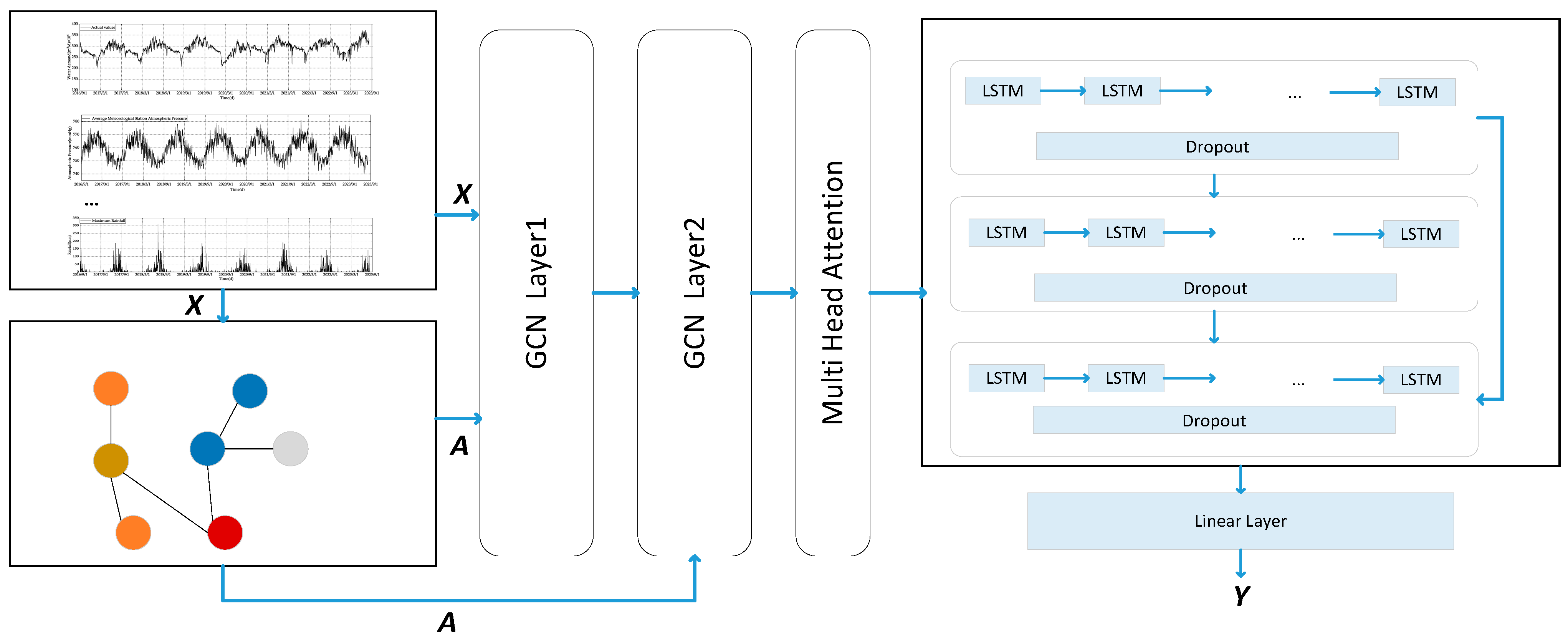
During data processing, the model initially applied the Prophet model to decompose water consumption data into four elements and then conducted anomaly detection and correction based on forecasting values. Additionally, min–max normalization was applied to the data to prevent overflow during computations, thus enhancing the prediction efficiency.

For spatial feature processing, this study input a total of 16 variables into the GCN and MIC analyses. These variables comprised climate data variables f₀–f₁₄ and water data variable y, collectively, designated as parameter X in the graph structure. Subsequently, the MIC was employed to uncover and visualize the indirect spatial relationships between meteorological data and water data. Furthermore, an adjacency matrix A was constructed to represent the similarity among features, with the dimension of matrix A being 16 × 16. To reduce complexity, a threshold τ was set to sparsify the adjacency matrix, zeroing out similarity values below τ. The GCN aggregates information from adjacent nodes into the water consumption node, providing spatially relevant features for water demand prediction. Considering the data’s scale and complexity, along with computational resources, the model limited the GCN layers to two [30]. The multi-head attention mechanism was applied to spatial features, dynamically calculating the importance of each position and executing weighted aggregation on the more significant parts.

For temporal feature processing, the extracted spatial features were input into a three-layer LSTM for water demand prediction. Considering that adding multiple LSTM layers could complicate the model and increase the risk of neural network degradation and overfitting, a residual connection was added between the first and third LSTM layers to mitigate the vanishing gradient problem. Additionally, dropout regularization was applied after each LSTM layer to decrease neuron interdependence; thereby, model complexity and the risk of overfitting were reduced. The final output was the water demand prediction result Y. Figure 5 outlines the complete model’s workflow.

3.1.1. Graph Convolutional Network (GCN)

The graph convolutional network [31] was introduced in 2017 by Kipf and Welling as a deep learning model specifically designed for processing graph data. The core advantage of GCN lies in its ability to adaptively adjust the representation of nodes, ensuring that each node sufficiently considers information from its neighboring nodes [32]. Due to its efficiency and flexibility in processing graph data, it has been applied in several domains, including traffic networks and urban planning [33,34], recommendation systems [35,36], and natural language processing [37]. The architecture of a GCN includes input, hidden, and output layers, as illustrated in Figure 6. In this architecture, each node’s features transform from $X$ to $Z$, while $Y$ represents the output result. The corresponding computation formulas are shown in Equations (3) and (4):

$$f({\mathrm{X}}_t^n,A)=Y,$$

(3)

$$A=\left[\begin{array}{cccc}1& a_{12}& \cdots & a_{1n}\\ a_{21}& 1& \ddots & ⋮\\ ⋮& \ddots & \ddots & a_{n-1n}\\ a_{n1}& \cdots & a_{nn-1}& 1\end{array}\right],$$

(4)

where ${\mathrm{X}}_t^n$ represents the input time series; n is the number of features in the meteorological and water consumption data; t is the length of the data; $Y$ is the output result; and $A$ denotes the adjacency matrix that represents the relationships among nodes.

3.1.2. Multi-Head Attention

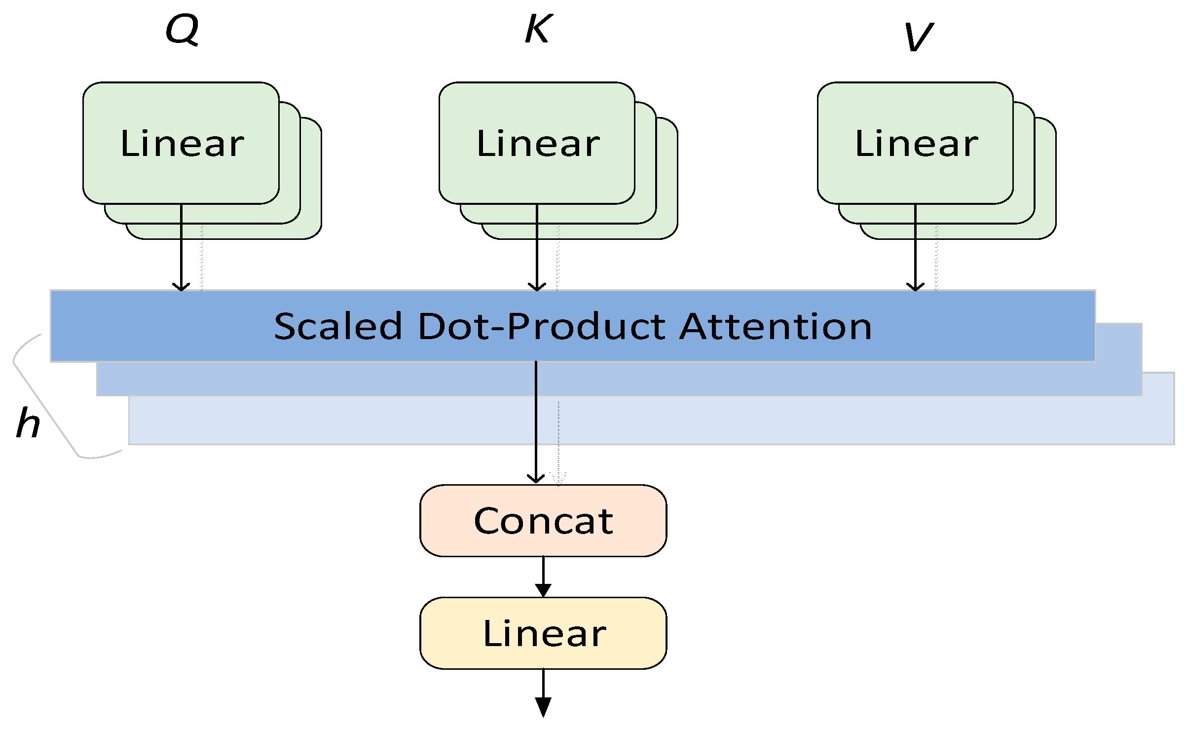
The multi-head attention mechanism is an advanced extension of the attention mechanism in the field of deep learning [38], effectively enhancing the extraction of key information from sequential data. In traditional attention mechanisms, there is usually only one weighted context vector to represent the information of the input sequence. In the multi-head attention, multiple sets of independent attention weights are employed. These independent sets can learn and capture semantic information at different levels, each generating a distinct context vector. These context vectors are then concatenated and subjected to a linear transformation to produce the final output. Figure 7 illustrates the structure of the multi-head attention mechanism, where $Q$, $K$, and $V$ represent the query, key, and value, respectively.

The processing procedure of the multi-head attention mechanism is depicted in Formulas (5) and (6):

$$MultiHead\left(Q,V,K\right)=Concat\left({\mathrm{head}}_1,\dots ,hea{d}_h\right)W^H,$$

(5)

$$hea{d}_i=Attention\left(Q{W}_i^Q,K{W}_i^K,V{W}_i^V\right),$$

(6)

where $W_i^Q$, $W_i^K$, $W_i^V$, and $W^H$ represent the parameter matrix and $hea{d}_i$ denotes the different head spaces. The $Concat$ operation is responsible for concatenating the computational results from different heads, followed by a linear transformation of the concatenated result.

3.1.3. Long Short-Term Memory (LSTM)

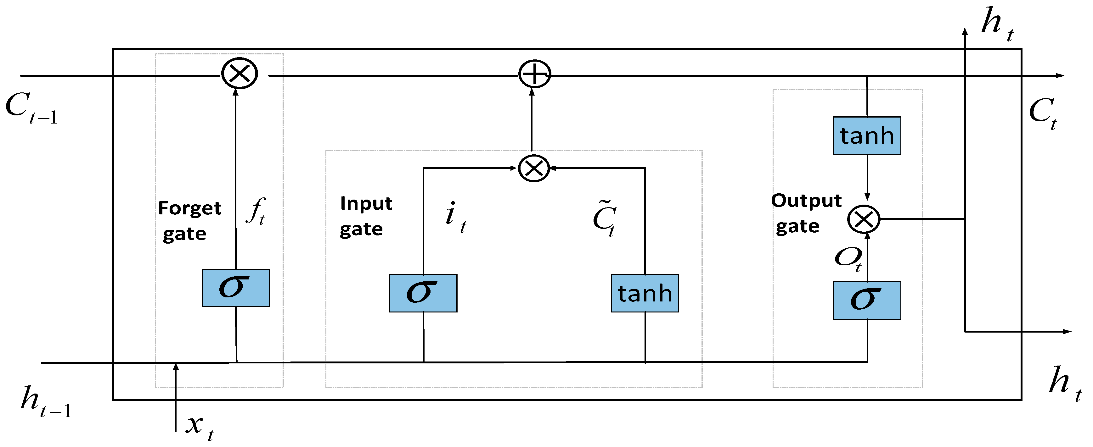
The LSTM [19,20] is designed to overcome problems of gradient vanishing and explosion encountered in traditional RNNs, making it more suitable for processing and predicting long-term dependencies in time series data. Unlike traditional RNNs, LSTM networks enhance their performance through the introduction of three gated structures, as depicted in Figure 8.

In Figure 8, the forget gate is responsible for deciding what information in the cell state should be retained or discarded. The input gate is responsible for deciding how much new input information should be stored into the cell state, and the output gate serves to decide the final output of the cell state.

The core operations of an LSTM network can be represented by the following equations:

$$f_t=\sigma \left(W_f\cdot \left[{\mathrm{h}}_{t-1},x_t\right]+b_f\right),$$

(7)

$$i_t=\sigma \left(W_i\cdot \left[{\mathrm{h}}_{t-1},x_t\right]+b_i\right),$$

(8)

$$\tilde{C}=\tanh (W_c\cdot \left[h_{t-1},x_t+b_c\right]),$$

(9)

$$C_t=f_t\ast C_{t-1}+i_t\ast {\tilde{C}}_t,$$

(10)

$$O_t=\sigma \left(W_o\cdot \left[{\mathrm{h}}_{t-1},x_t\right]+b_o\right),$$

(11)

$$h_t=O_t\ast \tanh (C_t),$$

(12)

where $C_{t-1}$ and $h_{t-1}$ are the cell state and output from the previous time step, respectively; $x_t$ is the input information at the current time step; $C_t$ and $h_t$ are the cell state and output at the present moment; $W$ represents the weight vectors for the gated structures, with $b$ as the bias vector.

3.2. Evaluation Criteria

In the comprehensive evaluation of predictive model performance, this study employed five key performance metrics. The root-mean-square error (RMSE) accentuates the impact of large errors, making it suitable for applications where significant deviations are of concern. The mean absolute error (MAE) applies to scenarios that are insensitive to outliers. The root-mean-square logarithmic error (RMSLE) focuses on the accuracy of the ratio between predicted and actual values, ideal for instances where precision in prediction outweighs the absolute magnitude. The mean absolute percentage error (MAPE) reflects the accuracy of predictions in percentage terms, suitable for evaluating relative errors. The coefficient of determination (R²) measures the variability in model predictions as it corresponds to the actual data, serving to assess the explanatory power of the model. Utilizing these metrics collectively offers a comprehensive perspective on model performance, with each metric highlighting different aspects of performance evaluation. The formulas for these indicators are as follows:

$$RMSE=\sqrt{\frac{{\displaystyle \sum _{i=1}^n{(y_i-{\widehat{y}}_i)}^2}}{n}},$$

(13)

$$MAE=\frac{1}{n}{\displaystyle \sum _{i=1}^n\left|{\widehat{y}}_i-y_i\right|},$$

(14)

$$RMSLE=\sqrt{\frac{1}{n}{\displaystyle \sum _{i=1}^n{(\ln ({\widehat{y}}_i+1)-\ln (y_i+1))}^2}},$$

(15)

$$MAPE=\frac{100\%}{n}{\displaystyle \sum _{i=1}^n\left|\frac{y_i-{\widehat{y}}_i}{y_i}\right|},$$

(16)

$$R^2=1-\frac{{\displaystyle {\sum }_i{({\widehat{y}}_i-y_i)}^2}}{{\displaystyle {\sum }_i{({\overline{y}}_i-y_i)}^2}},$$

(17)

where $n$ represents the entire count of data points; ${\widehat{y}}_i$ denotes the predicted value for the $i\text{-}\mathrm{th}$ data point; y_i matches the actual value; and ${\overline{y}}_i$ is the mean of all true observed values.

4. Results and Discussion

To verify the efficacy of the proposed model, this study conducted a sequence of comparative experiments. Section 4.1 details the parameter settings of all models, aiming to ensure consistency in experimental conditions. Section 4.2 presents a comparison of data processing outcomes. In Section 4.3, the methods of constructing the adjacency matrix are compared. Finally, in Section 4.4, the predictive performance of the proposed model is demonstrated through ablation experiments and comparisons with other prediction models. The experimental findings confirm the efficacy of the suggested model in predicting water demand.

4.1. Model Parameter Settings

To validate the performance of the proposed model, LSTM and convolutional neural network–long short-term memory network (CNN-LSTM) [4] were selected for comparison. In the domain of water demand forecasting, the LSTM network is capable of recognizing the long-term trends and cyclical changes in time series, serving as a powerful baseline model. The CNN-LSTM combines the advantages of CNN and LSTM networks, targeting the integrated processing of both spatial and temporal features within sequential data. The CNN layers autonomously extract spatial features from the input data, which are subsequently fed into the LSTM layer to capture temporal dependencies. All models developed for this study, including the comparative LSTM and CNN-LSTM models, were implemented within the Pytorch framework to ensure uniform experimental conditions.

The training process of the GCN-Att-LSTM model uses Adam’s optimizer [39] and mean-square-error (MSE) loss function to iteratively update the network parameters, thereby optimizing training efficiency. Since there are 15 climate data variables and water demand y in this paper, the input dimension is set to 16. In setting the lookback window, it is imperative to furnish each model with an equivalent volume of historical data for the learning process. Subsequently, through experimental assessment of each model’s predictive performance and complexity, it was determined that data from the preceding 10 days should be employed to forecast the subsequent day’s water demand. The detailed parameter settings for the GCN-Att-LSTM model, alongside the comparative LSTM and CNN-LSTM models, are listed in

Table 5. Model parameter settings.

Model	Parameter	Range	Result
CNN-LSTM	Out_channels	(32,64,128)	64
	Kernel_size	(2,3,5)	3
	LSTM_num_layers	(1,2,3)	1
	LSTM_hidden_size	(32,64,128,256)	64
	Batch_size	(16,32,64)	32
	Learning rate	[10−5,10−2]	10−3
	Lookback window	[7,10,14,20,30]	10
GCN-Att-LSTM	GCN_hidden_size	(132,64,128,256)	128
	GCN_out_size	(16,32,64)	16
	Num_heads	(4,8,16)	8
	LSTM_num_layer	(2,3)	2
	LSTM_hidden_size	(32,64,128)	128
	Dropout	(0.2,0.3,0.4)	0.3
	Learning rate	[10−5,10−2]	10−3
	Lookback window	[7,10,14,20,30]	10
LSTM	Hidden_size	(32,64,128)	64
	Num_layers	(1,2,3)	1
	Batch_size	(16,32,64)	16
	Learning rate	[10−5,10−2]	10−3
	Lookback window	[7,10,14,20,30]	10

. The optimal model parameter configuration was determined through cross-validation.

4.2. Data Processing Comparison

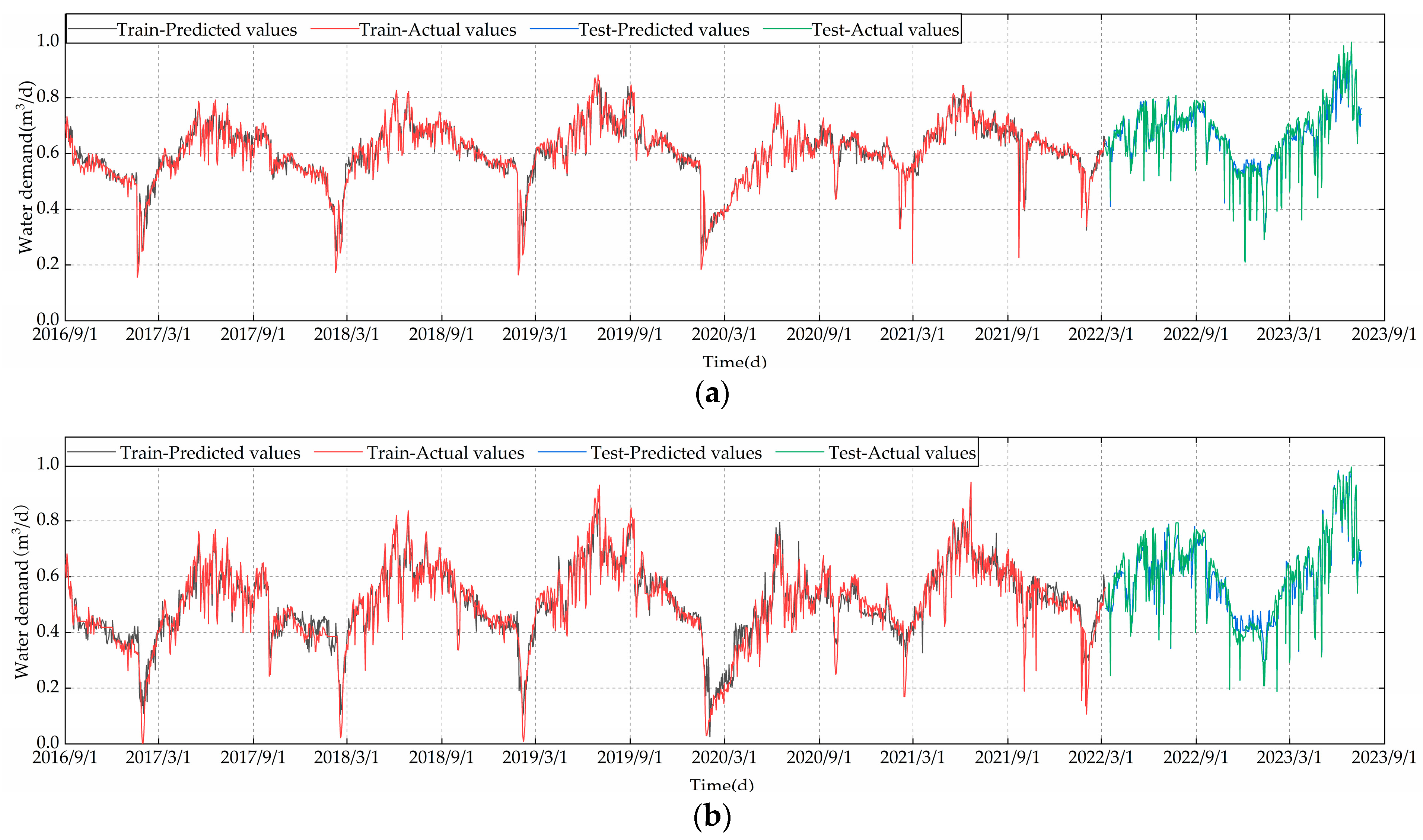
To demonstrate the effectiveness of data preprocessing with the Prophet model, this study implemented a comparative analysis, employing the 3σ [7] principle for detecting outliers and using the mean values of neighboring time points as fillers. The results of both processing were input into the constructed GCN-Att-LSTM model for training and testing, ensuring that all experiments were performed in the same computing environment. According to the prediction performance metrics presented in

Table 6. Comparison of results using different anomaly correction methods.

Performance Indicator	RMSE	MAE	RMSLE	MAPE (%)	R2
Prophet	0.03234	0.02231	0.02001	3.5652	0.92965
3σ	0.04886	0.03342	0.03211	6.70743	0.90239

, compared to the 3σ principle, the processing method of Prophet’s model reduced the RMSE, MAE, RMSLE, and MAPE by 1.652%, 1.111%, 1.21%, and 3.1409%, respectively, while increasing the R² value by 2.726%. These results highlight the superiority of the Prophet model in data processing. Figure 9a displays the results of data processing using the Prophet model, whereas Figure 9b shows the results of using the 3σ principle.

4.3. Comparison of Constructing Adjacency Matrices

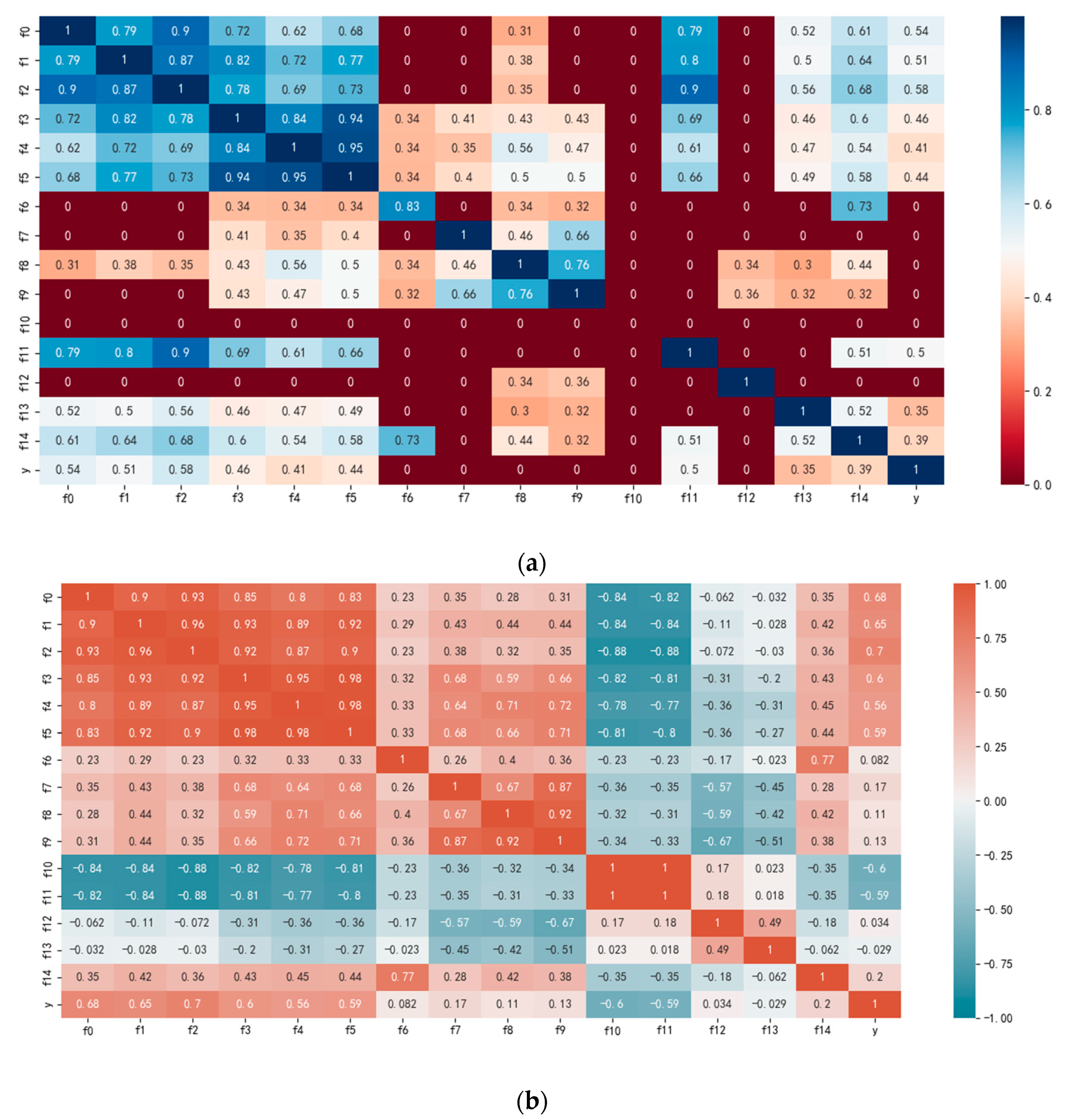
When constructing adjacency matrices to represent the similarity among input variables, conventional methods like Pearson correlation analysis are primarily suitable for detecting linear relationships. However, to capture complex functional relationships, especially nonlinear form, this paper used a grid-based information theory method—the maximal information coefficient (MIC) [40]. The MIC aims to reveal the full-range correlation between two variables. Compared to traditional Pearson correlation analysis, MIC exhibits significant advantages in computational complexity and robustness. To simplify model complexity, this study set a threshold τ, zeroing values in the adjacency matrix that are less than τ, thereby reducing unnecessary computational overhead. When the correlation score exceeds 0.3, it is considered that there is a significant temporal complex association between two variables, and hence τ is set to 0.3. The correlation results are shown in Figure 10, where f₀ to f₁₄ represent different meteorological data and y represents water usage. As seen in Figure 10a, f₀ to f₅, f₁₁, f₁₃, and f₁₄ have a higher correlation with water usage. To further validate the effectiveness of the MIC method, it was compared with Pearson correlation analysis, and the corresponding adjacency matrices were constructed, as shown in Figure 10b, displaying the positive and negative correlations between each variable and water usage.

In order to evaluate the effectiveness of the MIC in constructing the neighborhood matrix, matrices generated by two different methods were applied to the GCN-Att-LSTM model, with all training and testing executed in a unified computing environment. From the prediction results in

Table 7. Comparison of methods for constructing adjacency matrices.

Performance Indicator	RMSE	MAE	RMSLE	MAPE (%)	R2
MIC	0.03234	0.02231	0.02001	3.5652	0.92965
Pearson	0.04001	0.03324	0.02443	5.31143	0.89316

, the adjacency matrix constructed using the MIC method has reduced the RMSE, MAE, RMSLE, and MAPE by 0.767%, 1.093%, 0.442%, and 1.74623%, respectively, and has increased the R² by 3.649%. These results demonstrate the relative advantage of MIC in constructing the adjacency matrix. The prediction effect graph utilizing the MIC-constructed adjacency matrix is shown in Figure 9a. The prediction effect of constructing the adjacency matrix using Pearson correlation coefficient is shown in Figure 11.

4.4. Water Demand Model Comparison

To confirm the efficacy of the present model, LSTM and CNN-LSTM models were selected for comparative analysis. Additionally, a series of ablation experiments were executed to evaluate the contribution of each component within the present model. The model obtained by removing the multi-head attention mechanism from the complete GCN-Att-LSTM model was named GCN-LSTM, while simplifying the three-layer LSTM to a single-layer LSTM resulted in the GCN-Att-OneLSTM model. All models in this paper are designed to forecast water demand for the next day, with training and testing conducted in the same computing environment. Furthermore, an early stopping mechanism based on mean-square-error (MSE) was integrated into the model framework, with the patience parameter set to [5,10,15,20] and a significance threshold ranging from 1% to 0.01%. Through a series of experimental adjustments and cross-validation processes, it was determined that training should be halted if there is no more than a 0.1% decrease in MSE across 15 consecutive training epochs, as a measure to prevent overfitting.

Table 8. Comparison of different prediction model results.

Model	RMSE	MAE	RMSLE	MAPE (%)	R2	Epoch	Run Time for Each Epoch(s)
LSTM	0.05281	0.03966	0.03224	6.2832	0.85126	100	1.246
CNN-LSTM	0.04345	0.03304	0.02671	5.43400	0.87479	210	0.830
GCN-LSTM	0.04207	0.02890	0.02642	4.9185	0.88130	125	0.955
GCN-Att-OneLSTM	0.03724	0.02791	0.02310	4.5651	0.90614	125	1.102
GCN-Att-LSTM	0.03234	0.02231	0.02001	3.5652	0.92965	110	1.467

lists the detailed comparative data on the five performance indicators, training epochs, and the duration of each model’s training round.

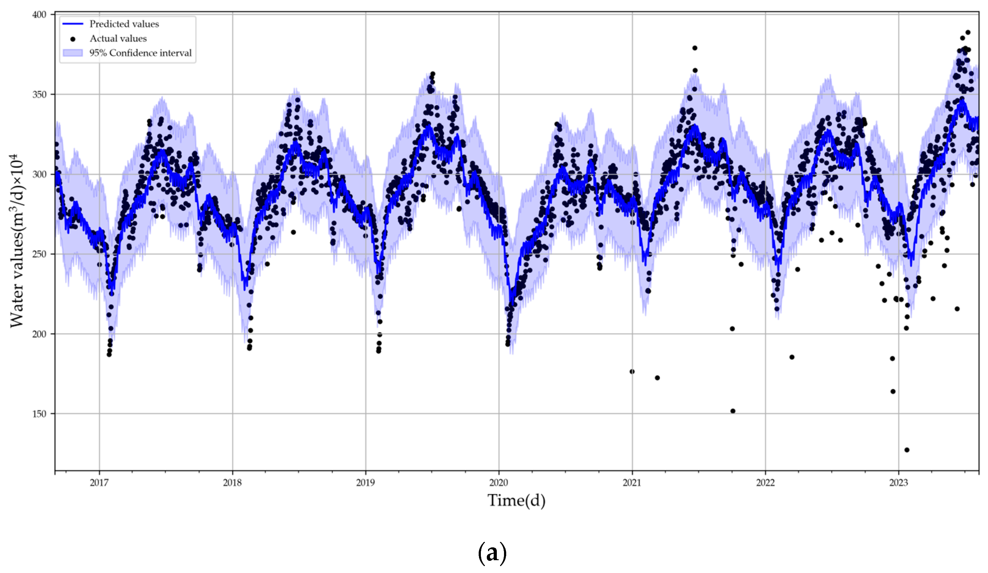
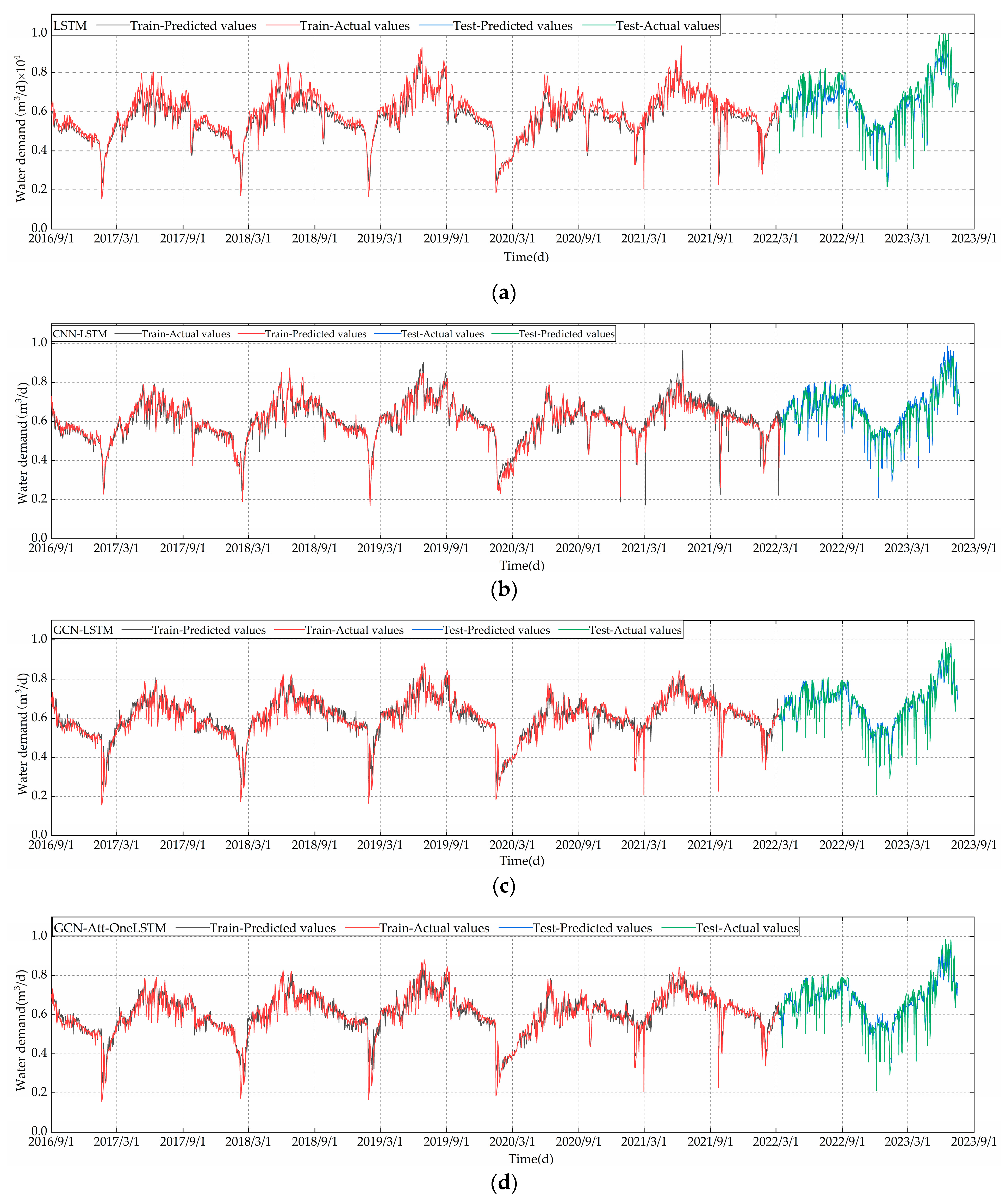
The data presented in Table 8 clearly indicate that the training times of the five models do not vary significantly. However, the predictive capability of the GCN-Att-LSTM model introduced in this study surpasses that of both the LSTM and CNN-LSTM models. This improvement is primarily attributed to the consideration of both temporal and spatial features among variables. This not only utilizes temporal information but also accounts for interactions within the spatial dimension of variables, thereby enhancing prediction accuracy. The outcomes of the ablation study further verify the contribution of each component to the model’s effectiveness, working together to accurately predict water demand. Additionally, to visually demonstrate the predictive efficacy of the models, the effect charts for each model are presented in Figure 12. The variation in MAE during the test is plotted in Figure 13, where the changes in prediction error for approximately 100 rounds are plotted in a single model, and the CNN-LSTM is plotted separately for ease of comparison. These visualizations aid in understanding the performance of the models.

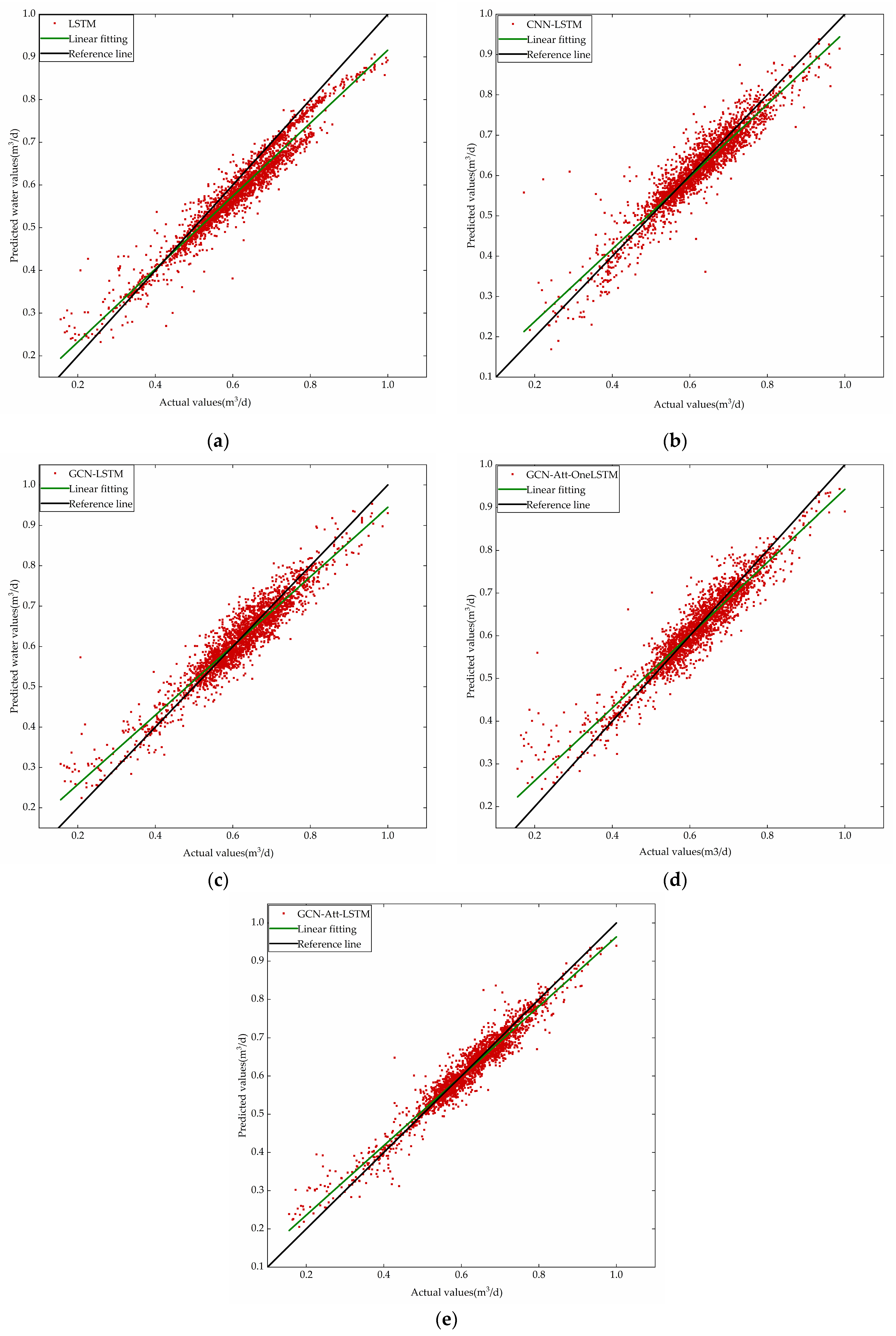
As observed from the figures above, the predictive trends of all models align with the actual data trends; however, the overall performance of our model is superior. Figure 12a demonstrates the efficacy of the LSTM model in forecasting short-term urban water usage. The LSTM model is capable of approximately following the water usage trends, indicating a certain level of predictive ability, but it may exhibit some deviations in capturing peak and trough values. As illustrated in Figure 12b, the CNN-LSTM model combines the feature extraction capabilities of convolutional neural networks with the sequential data processing advantages of LSTM. Comparison of the prediction curve with the real water consumption curve reveals the role of CNN in processing time series. Figure 12c shows the predictive effectiveness of the GCN-LSTM model, which integrates the spatial feature extraction capabilities of GCNs with the deep temporal feature processing of a three-layer LSTM. This model considers more profound correlations in the time series for prediction. The GCN-Att-OneLSTM model in Figure 12d integrates features from graph convolutional networks with the attention mechanism. It is observed that this model’s prediction curves show improvement over previous models, suggesting that the incorporation of the attention mechanism may have enhanced the model’s ability to capture the dynamic changes in water consumption. The GCN-Att-LSTM model, illustrated in Figure 12e, combines the attention mechanism with the three-layer LSTM, aiming to strengthen the model’s focus on key time points. The prediction curves more accurately simulate the fluctuations in actual water use than the previous models, especially in capturing peaks and sudden change points, potentially exhibiting higher accuracy and response sensitivity. It can also be seen from Figure 13 that the model achieves relatively good predictions. For a better assessment of each model’s capability in predicting short-term urban water demand, scatter plots for the five models are provided in Figure 14.

In these scatter plots, predicted values are represented by red dots, fitting curves by green lines, and black reference lines are utilized to assess the consistency between predicted and actual values. Comparative analysis reveals that the GCN-Att-LSTM model exhibits the highest consistency between predictions and actual values. The scatter distribution of the GCN-Att-LSTM model is more tightly clustered around the reference line, indicating its superior predictive accuracy compared to other models. This finding highlights the efficacy of the LSTM model combining GCN and attention mechanisms in addressing urban water demand prediction problems.

To comprehensively assess the performance of various models, this study further constructed violin plots for each model, as depicted in Figure 15. The height of the violin plots represents the full range of data distribution, while the width indicates the density of data points around specific values. The thick black line in the center of the plot marks the interquartile range of the data, with the white dot signifying the median. Comparative analysis demonstrates that the GCN-Att-LSTM and GCN-Att-OneLSTM models achieve the highest congruence with the actual data, as evidenced by their alignment in both the height and width with the actual data distribution. Although it is not easy to distinguish the significant difference between these two models from the violin plot, the data analyzed above confirm that the GCN-Att-LSTM model performs best.

5. Conclusions

Forecasting urban water demand is a critical aspect of environmental sustainability and urban infrastructure planning. Accurate short-term predictions are essential for optimizing water distribution, enhancing resource efficiency, and mitigating shortages. Traditional models often only consider the temporal features among variables, neglecting the spatial features that also impact urban water demand prediction. This study addresses the challenge of short-term urban water demand forecasting by proposing the GCN-Att-LSTM model. This model integrates spatial and temporal features among variables to improve the accuracy of urban water demand forecasts.

The quality of data directly influences the performance and generalization capability of predictive models. This study employs the Prophet model for anomaly detection and correction, which effectively captures the seasonality and cyclicality of water usage series, thus enhancing data quality. Moreover, the model integrates spatial and temporal features, analyzes the relationship between water usage and climate data using the maximum information coefficient (MIC), extracts spatial features with the graph convolutional network (GCN), and strengthens features related to water data with the multi-head attention mechanism. Lastly, a long short-term memory (LSTM) model is utilized to comprehensively explore the intrinsic features of time series data. The experiments demonstrated that the GCN-Att-LSTM model surpassed traditional LSTM and CNN-LSTM models in accuracy, reducing the MAPE by 1.868–2.718%. Ablation studies further clarified the contribution of each component within the model, confirming the significance of integrating spatial and temporal features.

The GCN-Att-LSTM model presented in this paper not only demonstrates the effectiveness of integrating multiple advanced techniques, but also introduces novel concepts and approaches for future urban water usage forecasting. By fusing spatial and temporal features among variables, it can more accurately decipher complex patterns in water use data, thus improving the accuracy of water demand prediction. However, like many complex models, the GCN-Att-LSTM possesses a black-box nature, limiting its interpretability. Future research should further explore this model, incorporating additional influencing factors to improve its robustness, accuracy, and predictive capability.

References

1. Chen, F. Study on the Circular Utilization Patterns of City Water Resources. In Proceedings of the 2015 International Conference on Applied Science and Engineering Innovation, Jinan, China, 30–31 August 2015; pp. 1664–1669. [Google Scholar]
2. Chen, X.; Xu, Q.; Cai, J. Research on the urban water resources carrying capacity by using system dynamics simulation. Hydrol. Res. 2023, 54, 418–434. [Google Scholar] [CrossRef]
3. Guo, J.; Sun, H.; Du, B. Multivariable time series forecasting for urban water demand based on temporal convolutional network combining random forest feature selection and discrete wavelet transform. Water Resour. Manag. 2022, 36, 3385–3400. [Google Scholar] [CrossRef]
4. Zhou, S.; Guo, S.; Du, B.; Huang, S.; Guo, J. A Hybrid Framework for Multivariate Time Series Forecasting of Daily Urban Water Demand Using Attention-Based Convolutional Neural Network and Long Short-Term Memory Network. Sustainability 2022, 14, 11086. [Google Scholar] [CrossRef]
5. Hu, S.; Gao, J.; Zhong, D.; Deng, L.; Ou, C.; Xin, P. An innovative hourly water demand forecasting preprocessing framework with local outlier correction and adaptive decomposition techniques. Water 2021, 13, 582. [Google Scholar] [CrossRef]
6. Ghannam, S.; Hussain, F. Comparison of deep learning approaches for forecasting urban short-term water demand a Greater Sydney Region case study. Knowl.-Based Syst. 2023, 275, 110660. [Google Scholar] [CrossRef]
7. Du, B.; Zhou, Q.; Guo, J.; Guo, S.; Wang, L. Deep learning with long short-term memory neural networks combining wavelet transform and principal component analysis for daily urban water demand forecasting. Expert Syst. Appl. 2021, 171, 114571. [Google Scholar] [CrossRef]
8. Pu, Z.; Yan, J.; Chen, L.; Li, Z.; Tian, W.; Tao, T.; Xin, K. A hybrid Wavelet-CNN-LSTM deep learning model for short-term urban water demand forecasting. Front. Environ. Sci. Eng. 2023, 17, 22. [Google Scholar] [CrossRef]
9. Peng, Y.; Xiao, Y.; Fu, Z.; Dong, Y.; Zheng, Y.; Yan, H.; Li, X. Precision irrigation perspectives on the sustainable water-saving of field crop production in China: Water demand prediction and irrigation scheme optimization. J. Clean. Prod. 2019, 230, 365–377. [Google Scholar] [CrossRef]
10. Anele, A.O.; Hamam, Y.; Abu-Mahfouz, A.M.; Todini, E. Overview, comparative assessment and recommendations of forecasting models for short-term water demand prediction. Water 2017, 9, 887. [Google Scholar] [CrossRef]
11. Peng, H.; Wu, H.; Wang, J.; Dede, T. Research on the prediction of the water demand of construction engineering based on the BP neural network. Adv. Civ. Eng. 2020, 2020, 8868817. [Google Scholar] [CrossRef]
12. Li, H.; Zhang, C.; Miao, D.; Wang, T.; Feng, Y.; Fu, H.; Zhao, M. Water demand prediction of grey markov model based on GM (1, 1). In Proceedings of the 2016 3rd International Conference on Mechatronics and Information Technology, Toronto, ON, Canada, 2–3 August 2016; pp. 524–529. [Google Scholar]
13. Yang, B.; Zheng, W.; Ke, X. Forecasting of industrial water demand using case-based reasoning—A case study in Zhangye City, China. Water 2017, 9, 626. [Google Scholar] [CrossRef]
14. Jiang, B.; Mu, T.; Zhao, M.; Shen, D.; Wang, L. Study of PSO-SVM model for daily water demand prediction. In Proceedings of the 2017 5th International Conference on Mechatronics, Materials, Chemistry and Computer Engineering (ICMMCCE 2017), Chongqing, China, 24–25 July 2017; pp. 408–413. [Google Scholar]
15. Mensik, P.; Marton, D. Hybrid optimization method for strategic control of water withdrawal from water reservoir with using support vector machines. Procedia Eng. 2017, 186, 491–498. [Google Scholar] [CrossRef]
16. Villarin, M.C.; Rodriguez-Galiano, V.F. Machine learning for modeling water demand. J. Water Resour. Plan. Manag. 2019, 145, 04019017. [Google Scholar] [CrossRef]
17. Brentan, B.M.; Luvizotto, E., Jr.; Herrera, M.; Izquierdo, J.; Pérez-García, R. Hybrid regression model for near real-time urban water demand forecasting. J. Comput. Appl. Math. 2017, 309, 532–541. [Google Scholar] [CrossRef]
18. Eslamian, S.A.; Li, S.S.; Haghighat, F. A new multiple regression model for predictions of urban water use. Sustain. Cities Soc. 2016, 27, 419–429. [Google Scholar] [CrossRef]
19. Mu, L.; Zheng, F.; Tao, R.; Zhang, Q.; Kapelan, Z. Hourly and daily urban water demand predictions using a long short-term memory based model. J. Water Resour. Plan. Manag. 2020, 146, 05020017. [Google Scholar] [CrossRef]
20. Kühnert, C.; Gonuguntla, N.M.; Krieg, H.; Nowak, D.; Thomas, J.A. Application of LSTM networks for water demand prediction in optimal pump control. Water 2021, 13, 644. [Google Scholar] [CrossRef]
21. Al-Ghamdi, A.B.; Kamel, S.; Khayyat, M. A Hybrid Neural Network-based Approach for Forecasting Water Demand. Comput. Mater. Contin. 2022, 73, 1366–1383. [Google Scholar] [CrossRef]
22. Zubaidi, S.L.; Ortega-Martorell, S.; Al-Bugharbee, H.; Olier, I.; Hashim, K.S.; Gharghan, S.K.; Al-Khaddar, R. Urban water demand prediction for a city that suffers from climate change and population growth: Gauteng province case study. Water 2020, 12, 1885. [Google Scholar] [CrossRef]
23. Li, J.; Song, S. Urban Water Consumption Prediction Based on CPMBNIP. Water Resour. Manag. 2023, 37, 5189–5213. [Google Scholar] [CrossRef]
24. Hu, P.; Tong, J.; Wang, J.; Yang, Y.; de Oliveira Turci, L. A hybrid model based on CNN and Bi-LSTM for urban water demand prediction. In Proceedings of the 2019 IEEE Congress on evolutionary computation (CEC), Museum of New Zealand Te Papa Tongarewa, Wellington, New Zealand, 10–13 June 2019; pp. 1088–1094. [Google Scholar]
25. Zheng, H.; Liu, Y.; Wan, W.; Zhao, J.; Xie, G. Large-scale prediction of stream water quality using an interpretable deep learning approach. J. Environ. Manag. 2023, 331, 117309. [Google Scholar] [CrossRef]
26. Wang, H.; Zhang, L.; Wu, R.; Zhao, H. Enhancing Dissolved Oxygen Concentrations Prediction in Water Bodies: A Temporal Transformer Approach with Multi-Site Meteorological Data Graph Embedding. Water 2023, 15, 3029. [Google Scholar] [CrossRef]
27. Zanfei, A.; Brentan, B.M.; Menapace, A.; Righetti, M.; Herrera, M. Graph convolutional recurrent neural networks for water demand forecasting. Water Resour. Res. 2022, 58, e2022WR032299. [Google Scholar] [CrossRef]
28. Wang, Y.; Huang, Y.; Xiao, M.; Zhou, S.; Xiong, B.; Jin, Z. Medium-long-term prediction of water level based on an improved spatio-temporal attention mechanism for long short-term memory networks. J. Hydrol. 2023, 618, 129163. [Google Scholar] [CrossRef]
29. Fronzi, D.; Narang, G.; Galdelli, A.; Pepi, A.; Mancini, A.; Tazioli, A. Towards Groundwater-Level Prediction Using Prophet Forecasting Method by Exploiting a High-Resolution Hydrogeological Monitoring System. Water 2024, 16, 152. [Google Scholar] [CrossRef]
30. Chen, Z.; Xu, J.; Peng, T.; Yang, C. Graph convolutional network-based method for fault diagnosis using a hybrid of measurement and prior knowledge. IEEE Trans. Cybern. 2021, 52, 9157–9169. [Google Scholar] [CrossRef] [PubMed]
31. Kipf, T.N.; Welling, M. Semi-supervised classification with graph convolutional networks. arXiv 2016, arXiv:1609.02907. [Google Scholar]
32. Zhou, J.; Cui, G.; Hu, S.; Zhang, Z.; Yang, C.; Liu, Z.; Wang, L.; Li, C.; Sun, M. Graph neural networks: A review of methods and applications. AI Open 2020, 1, 57–81. [Google Scholar] [CrossRef]
33. Peng, D.; Zhang, Y. MA-GCN: A Memory Augmented Graph Convolutional Network for traffic prediction. Eng. Appl. Artif. Intell. 2023, 121, 106046. [Google Scholar] [CrossRef]
34. Feng, R.; Cui, H.; Feng, Q.; Chen, S.; Gu, X.; Yao, B. Urban Traffic Congestion Level Prediction Using a Fusion-Based Graph Convolutional Network. IEEE Trans. Intell. Transp. Syst. 2023, 24, 14695–14705. [Google Scholar] [CrossRef]
35. Chang, Y.; Zhou, W.; Wen, J. IHG4MR: Interest-oriented heterogeneous graph for multirelational recommendation. Expert Syst. Appl. 2023, 228, 120321. [Google Scholar] [CrossRef]
36. Yin, Y.; Li, Y.; Gao, H.; Liang, T.; Pan, Q. FGC: GCN-Based Federated Learning Approach for Trust Industrial Service Recommendation. IEEE Trans. Ind. Inform. 2022, 19, 3240–3250. [Google Scholar] [CrossRef]
37. Yang, X.; Wang, X.; Wang, N.; Gao, X. Address the unseen relationships: Attribute correlations in text attribute person search. IEEE Trans. Neural Netw. Learn. Syst. 2023, 1–11. [Google Scholar] [CrossRef]
38. Zhang, Y.M.; Wang, H. Multi-head attention-based probabilistic CNN-BiLSTM for day-ahead wind speed forecasting. Energy 2023, 278, 127865. [Google Scholar] [CrossRef]
39. Kingma, D.P.; Ba, J. Adam: A method for stochastic optimization. arXiv 2014, arXiv:1412.6980. [Google Scholar]
40. Reshef, D.N.; Reshef, Y.A.; Finucane, H.K.; Grossman, S.R.; McVean, G.; Turnbaugh, P.J.; Sabeti, P.C. Detecting novel associations in large data sets. Science 2011, 334, 1518–1524. [Google Scholar] [CrossRef] [PubMed]
Figure 1. (a) Water usage data; (b) meteorological station atmospheric pressure; (c) maximum rainfall; (d) dew point; (e) temperature; (f) average wind speed.
Water 16 00831 g001aWater 16 00831 g001b
Figure 2. Annual water usage data from 2017 to 2022.
Water 16 00831 g002
Figure 3. Prophet model effect plots: (a) prediction plot; (b) outlier detection plot.
Water 16 00831 g003aWater 16 00831 g003b
Figure 4. Data processing result.
Water 16 00831 g004
Figure 5. GCN-Att-LSTM model structure.
Water 16 00831 g005
Figure 6. Graph convolutional network.
Water 16 00831 g006
Figure 7. Structure of the multi-head attention.
Water 16 00831 g007
Figure 8. LSTM neural network structure.
Water 16 00831 g008
Figure 9. Predicted results: (a) Prophet data processing; (b) 3σ rule data processing.
Water 16 00831 g009
Figure 10. Constructing adjacency matrix: (a) MIC correlation among variables; (b) Pearson correlation among variables.
Water 16 00831 g010
Figure 11. Prediction result of Pearson adjacency matrix.
Water 16 00831 g011
Figure 12. Predicted effects of each model: (a) LSTM prediction result; (b) CNN-LSTM prediction result; (c) GCN-LSTM prediction result; (d) GCN-Att-OneLSTM prediction result; (e) GCN-Att-LSTM prediction result.
Water 16 00831 g012aWater 16 00831 g012b
Figure 13. MAE test error variation: (a) GCN-Att-LSTM, GCN-LSTM, GCN-Att-OneLSTM and LSTM error variation; (b) CNN-LSTM error variation.
Water 16 00831 g013
Figure 14. Scatter plots for the actual and prediction values: (a) LSTM scatter plot; (b) CNN-LSTM scatter plot; (c) GCN-LSTM scatter plot; (d) GCN-Att-OneLSTM scatter plot; (e) GCN-Att-LSTM scatter plot.
Water 16 00831 g014
Figure 15. Violin plot for the actual and prediction values.
Water 16 00831 g015