An Improved One-Line Evolution Formulation for the Dynamic Shoreline Planforms of Embayed Beaches

Abstract

In this paper, an improved one-line evolution formulation is proposed and derived for the dynamic shoreline planforms of embayed beaches. Although embayed sandy beaches can perform several functions, serving as leisure spots and areas of coastal protection, shoreline advances and retreats occur continuously as a result of many natural forces, such as winds, waves, currents, tides, etc. The one-line evolution formulation for dynamic shoreline planforms based on the polar coordinate can be adopted to simulate high-planform-curvature shorelines and achieve better stability and simplicity in comparison with other description coordinates. While the polar coordinate and rectangular control volume are adopted to derive the one-line evolution formulation for dynamic shoreline planforms, the difference between the radial direction of the polar coordinate and the normal direction of the shoreline segment may result in inaccurate predictions of shoreline movements. In this study, a correction coefficient, which can adjust the influence of these two misaligned directions, is derived and included in the one-line evolution formulation, which is based on the polar coordinate. Thus, by considering the correction coefficient, an improved one-line evolution formulation for dynamic shoreline planforms of crenulate-shaped bays is proposed in this paper. Some numerical examples are provided to verify the merits of the proposed improved one-line evolution formulation. Moreover, the proposed numerical approach is applied to simulate the dynamic movements of the shoreline in Taitung—the southeastern part of Taiwan—and the effectiveness of the proposed formulation in solving realistic engineering applications is evidently verified.

1. Introduction

It is well known that in the past century, coastal protection via conventional engineering methods for solid structures has greatly contributed to protecting human property, homeland conservation and harbor construction. In several theoretical studies and practical engineering applications, researchers and engineers have proposed many methods and a variety of coastal structures [1] for protection of the coastal area. However, it is noted that shoreline advances and shoreline retreats still occur continuously under the interactions of many day-and-night natural forces, such as waves, currents, tides, winds, etc. Several failure cases of engineering structures for coastal protection against natural forces may imply that the desired functions of man-made structures for coastal protection are possibly limited [2,3]. While the limitations of conventional engineering methods for solid structures against natural forces are noted extensively, researchers and engineers are looking for other ways to protect the coastal zone. Jetties, groins and breakwaters are some of the above-mentioned structures, which can efficiently guide and manage natural forces, as well as adequately protect the coastal area. Many investigations, such as Refs. [4,5,6], have already verified the expected functions of shoreline protection by properly adopting jetties, groins and breakwaters.

One of the engineering approaches utilizing breakwaters is headland control. The idea of headland control comes from two protruding capes in nature. After the refraction and diffraction of water waves in the nearshore area, a region of stable water will develop between these two capes. Therefore, the sediment could settle down and form a beach, which is called a crenulate-shaped bay. As a result of more studies in this domain, scholars have found that land-connected islands are easily formed on reefs near the shoreline in the coastal zone. It is worth mentioning that breakwaters, land-connected islands and capes have the same function, which is to gradually form embayed beaches in the sheltered area. Through this observation, it is expected that breakwaters can have the same function as capes in forming embayed beaches by guiding and managing natural forces. Therefore, on the basis of headland control, the engineering approaches to breakwaters are widely adopted and implemented in numerous sites of coastal protection. Features of crenulate-shaped bays were first proposed by Hsu and Evans [7], and the planform of an embayed beach was described by a logarithmic spiral. Following a pioneer study in Ref. [8] on shoreline shape in a static equilibrium, many researchers have devoted a lot of attention to developing the description methods for shoreline planforms in a static equilibrium, such as the method based on the second-order polynomial. Consequently, these methods have been implemented in many realistic engineering applications [7,9]. The commercial software MEPBAY 3.0 has been developed to calculate shoreline planforms in a static equilibrium using polynomials, and it is widely used in real engineering projects in coastal protection. Although studies on shoreline planform calculation in a static equilibrium have been proposed and examined over the past decades, it is obvious that the weather conditions, wave fields, currents and tides in the study areas are very different from one day to the next, which implies that the shoreline profile should change continuously. Hence, in addition to the methods for shoreline planform calculation in a static equilibrium, it is more important and necessary to develop numerical methods for accurately and efficiently simulating the dynamic movements of shoreline planforms. This is the principal objective of this paper, i.e., the development of an improved one-line evolution formulation for dynamic shoreline planforms of embayed beaches.

In order to describe dynamic shoreline planforms, many methods have recently been proposed. One of the most popular methods for describing dynamic shoreline planforms is the one-line model, in which the spatial position of the shoreline is described by a function of one independent variable, as proposed in Ref. [10]. Previous studies have shown that the most straightforward way of representing the shoreline is to adopt the Cartesian coordinate system. This method has been widely applied since it was proposed [11,12]. The most well-known applications in commercial software are GenCade v1.34 in SMS and GENESIS in CEDAS [13], which were developed using the Cartesian coordinate system to simulate the dynamic movements of shoreline planforms. Due to the simplicity of GenCade or GENESIS, these commercial packages are very popular and used in many engineering projects. Although the Cartesian-coordinate-based evolution formulation in GenCade and GENESIS is very simple and efficient, it is well known that it is very difficult to simulate a high-planform-curvature shoreline. In order to overcome this difficulty, in 2010, Weesakul et al. [14] proposed a numerical scheme by adopting both the Cartesian coordinate system and the polar coordinate system. In the hooked zone, which is the lee of the headland, the shoreline portion is depicted by the polar coordinate system, while in the unhooked zone, which will be directly attacked by incident waves, the shoreline portion is depicted by the Cartesian coordinate system. Based on numerical comparisons, it is verified that the hybrid formulation, based on both coordinate systems, can accurately describe the dynamic movements of shoreline planforms of embayed beaches. However, in the hybrid formulation proposed in Ref. [14], the connection between the two coordinate systems may possibly result in an unstable simulation. Moreover, the quadratic term in the evolution formulation for the hooked zone will require more computer resources during numerical simulation. It is apparent that the connection along the interface of the two coordinates and the calculations of the square term and the square root in the hybrid formulation proposed in Ref. [14] will definitely require more computer resources in comparison with our proposed model. In 2022, Tao et al. [15] proposed a novel evolution formulation using the polar coordinate system both in the hooked zone and the unhooked zone, so as to eliminate the possible weakness in the hybrid formulation [14]. The polar-coordinate-based formulation is derived using the conservation law of mass for sediment and adopting the rectangular control volume, so that the interface problem—induced by the two coordinate systems—and the problem of the computer resources required—caused by the quadratic term—in the hybrid formulation can truly be overcome. Based on the numerical results and comparisons in Ref. [15], the polar-coordinate-based evolution formulation can accurately and efficiently simulate the dynamic shoreline planform of an embayed beach.

An improved evolution formulation is derived in this paper by considering the correction coefficient, so as to accurately simulate the dynamic movements of shoreline planforms. With the help of the correction coefficient proposed in this paper, the mathematical model and numerical scheme for dynamic shoreline planforms are more sound and correct than those in our previous study [15].

The structure of this paper is organized as follows. A discussion of the relevant literature and the motivation of this study is provided in the first section. The proposed improved evolution formulation and the correction coefficient are derived in the second section, while two numerical examples are presented in the third section to verify the merits of the proposed one-line model. In the fourth section, the engineering application is adopted to verify the applicability of the proposed improved evolution formulation. In the final section, some concluding remarks and a discussion are provided to summarize the contributions of this paper.

2. Shoreline Model for Dynamic Planforms

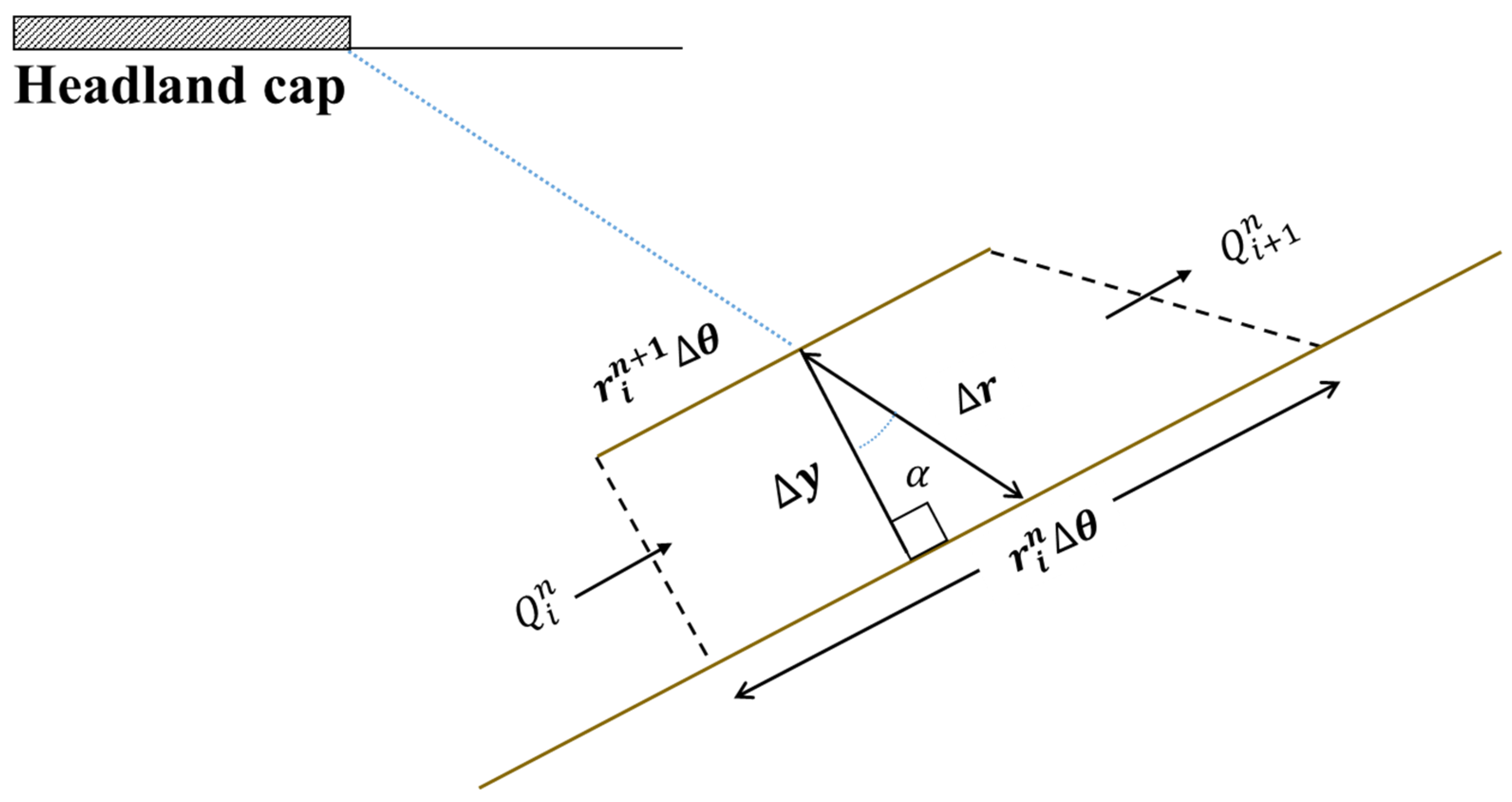
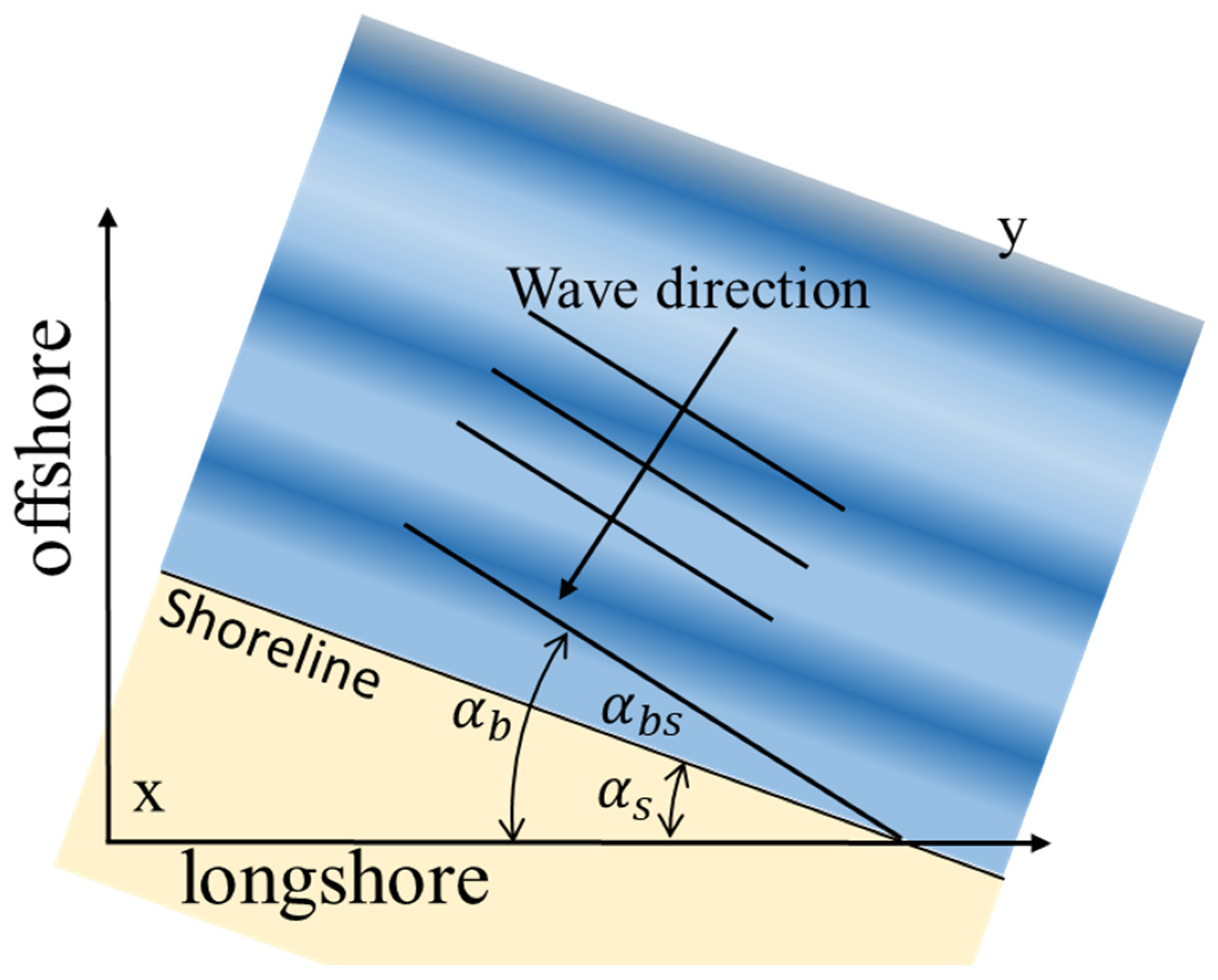
2.1. The Proposed Improved Evolution Formulation

In this paper, an improved evolution formulation for dynamic shoreline planforms is proposed on the basis of the polar coordinate and rectangular control volume. The proposed improved evolution formulation is developed based on the Cartesian-coordinate-based one-line shoreline models described by the GENESIS and GenCade software. Thus, the proposed improved evolution formulation follows the same assumptions in the GENESIS and GenCade software. The basic assumptions for the proposed improved evolution formulation are listed as follows:

• The shape of the beach profile remains constant.
• The shoreward and seaward depth limits of the profile are constant; meanwhile, sand is transported alongshore via the action of breaking waves.
• The detailed structure of nearshore circulation is ignored.
• There is a long-term trend in shoreline evolution.

Based on the above-mentioned assumptions, an improved evolution formulation for dynamic shoreline planforms is derived in this section by adopting the conservation law of mass, i.e., sediment conservation. In order to avoid the possible drawbacks resulting from the Cartesian coordinate or a combination of the Cartesian coordinate with the polar coordinate, the proposed formulation adopts the polar coordinate to describe the whole shoreline, which includes the hooked zone and the unhooked zone. A schematic diagram of the shoreline planform of an embayed sandy bay is depicted in Figure 1. Moreover, one headland is presented, and the origin of the coordinate system is placed at the tip of upcoast headland. The position vectors both in the Cartesian coordinate and the polar coordinate are presented in Figure 1. Therefore, the position vectors in the two coordinate systems can be related to each other using the following equation:

$$\left\{\begin{array}{c}x=rcos\theta \\ y=rsin\theta \end{array}\right.$$

(1)

where $(x,y)$ and $(r,\theta )$ are, respectively, the position vectors in the Cartesian coordinate and the polar coordinate.

In Figure 1, it is obvious that the entire shoreline from the headland to the downcoast control point is divided into $m$ segments. In the middle of each segment, the radial positions of the central points are denoted by $\{r_i{\}}_{i=1}^m$, representing the distance between the central node of the $i^{th}$ shoreline segment and the control point of the upcoast headland. In Figure 1, the shoreline segments both in the hooked zone and the unhooked zone are represented using the polar coordinate, so as to ensure the simplicity and stability of the computer simulation.

Since the entire shoreline in Figure 1 is divided into $m$ adjacent segments, each shoreline segment will experience shoreline retreats or shoreline advances. For a clear description, the $i^{th}$ shoreline segment is depicted in Figure 2. The $i^{th}$ shoreline segments in two sequential time steps, which are the $n^{th}$ time step and the ${(n+1)}^{th}$ time step, are presented. The spatial position of the ith shoreline segment in the $n^{th}$ time step is denoted by $r_i^n$, while the spatial position of the ith shoreline segment in the ${(n+1)}^{th}$ time step is denoted by $r_i^{n+1}$. $∆t=(t^{n+1}-t^n)$ is the time increment between the two sequential time steps. The longshore sediment transport between the $i^{th}$ shoreline segment and ${(i-1)}^{th}$ shoreline segment is denoted by $Q_i^n$, while the longshore sediment transport between the $i^{th}$ shoreline segment and ${(i+1)}^{th}$ shoreline segment is denoted by $Q_{i+1}^n$. The difference between these two longshore sediment transports within one time step ${(Q}_{i+1}^n-Q_i^n)$ will lead to shoreline advances or shoreline retreats. During the process of numerical simulation, the closure depth $D_s$ is set as a constant value because one assumption is that the beach profile remains constant.

In Figure 2, the plane area resulting from shoreline retreats or advances is denoted by $∆\mathrm{A}$ and represents the control volume for evolution formulation. The plane area $∆\mathrm{A}$ is surrounded by four boundary segments. Thus, the volume change in the $i^{th}$ shoreline segment between two sequential time steps $∆\mathrm{V}$ can be illustrated as follows:

$$∆V=∆Q∆t$$

(2)

$$∆V=D_s∆A$$

(3)

In Equation (3), the volume change in the $i^{th}$ shoreline segment $∆\mathrm{V}$ is represented by the differences in longshore sediment transport along two adjacent interfaces $∆Q={(Q}_{i+1}^n-Q_i^n)$. Meanwhile, the volume change in the $i^{th}$ shoreline segment $∆\mathrm{V}$ can be expressed via multiplication of the plane area $∆\mathrm{A}$ by closure depth $D_s$ in Equation (3). Since Equations (2) and (3) describe the same volume change in the $i^{th}$ shoreline segment $∆\mathrm{V}$ from different viewpoints, these two equations can be combined with each other.

In GENESIS, the one-line formulation for dynamic shoreline planforms of crenulate-shaped bays is derived using the Cartesian coordinate and rectangular control volume. In our previous study [15], the rectangular control volume was adopted both in the hooked zone and the unhooked zone. Therefore, the rectangular control volume was used in the polar-coordinate-based formulation. In addition, the control volume in Figure 2 is approximated by a rectangle, and the plane area $∆\mathrm{A}$ can be demonstrated as follows:

$$D_s∆A=∆Q∆t$$

(4)

$$∆A=(r_i^n∆\theta )∆\mathrm{r}=(r_i^n∆\theta )(r^{n+1}-r^n)$$

(5)

where $∆\theta$ is the increment in the angular direction of the polar coordinate system. In Equation (5), the first term on the right-hand side $(r_i^n∆\theta )$ depicts the approximation of the length of an arc, which denotes the length of the rectangular control volume. Moreover, the second term ($r^{n+1}-r^n$) on the right-hand side of Equation (5) shows the width of rectangular control volume. Once the width and the length of the rectangle are determined, a combination of Equations (3) and (5) can result in the following equation:

$$D_s\left(r_i^n∆\theta \right)\left(r^{n+1}-r^n\right)=∆Q∆t$$

(6)

Geometrically speaking, the control volume in the hooked zone is more like an annular sector, and the control volume in the unhooked zone is similar to a parallelogram if the polar coordinate system is adopted to describe the entire shoreline. In our previous study, the central point in the middle of the ith shoreline segment in the $n^{th}$ time step was moved along the radial direction ($r$ direction), which is obvious in Figure 2. If we carefully observe the control volume, it can be found that the radial direction of the polar coordinate system and the normal direction of the ith shoreline segment are very similar to each other for the shoreline in the hooked zone. However, for the shoreline in the unhooked zone, the radial direction of the polar coordinate system is very different from the normal direction of the ith shoreline segment. The inconsistency in the radial direction and the normal direction should be included in the one-line formulation of the dynamic shoreline planform of a crenulate-shaped bay. In this paper, we derive an improved evolution formulation by adding a correction coefficient of these two directions.

In Figure 3, it is obvious that the radial direction of the polar coordinate system and the normal direction of the ith shoreline segment are distinct. The ith shoreline segment in the $n^{th}$ time step will be moved to the ith shoreline segment in the ${(n+1)}^{th}$ time step along the normal direction of the shoreline segment. Therefore, the distance between the two shoreline segments in the $n^{th}$ time step and the ${(n+1)}^{th}$ time step is denoted by $∆\mathrm{y}$. The relation between $∆\mathrm{y}$ and $∆\mathrm{r}=\left(r^{n+1}-r^n\right)$ can be established and found in Figure 3.

$$∆\mathrm{y}=(∆\mathrm{r})\mathrm{c}\mathrm{o}\mathrm{s}\mathsf{\alpha }=\left(r_i^{n+1}{-r}_i^n\right)\mathrm{c}\mathrm{o}\mathrm{s}\mathsf{\alpha }$$

(7)

where $\mathsf{\alpha }$ is the angle between $∆\mathrm{y}$ and $∆\mathrm{r}$. Since the width of the rectangular control volume is described by $∆\mathrm{y}$ instead of $∆\mathrm{r}$ in Figure 3, the plane area in Equation (3) and Equation (3) should be adjusted as

$$∆A=(r_i^n∆\theta )∆\mathrm{y}$$

(8)

$$D_s∆A=D_s(r_i^n∆\theta )∆\mathrm{y}=D_s\left(r_i^n∆\theta \right)\left(r^{n+1}-r^n\right)\mathrm{c}\mathrm{o}\mathrm{s}\mathsf{\alpha }=∆Q∆t$$

(9)

The improved one-line evolution formulation for the dynamic shoreline planform of a crenulate-shaped bay can be derived in Equation (3):

$$r_i^{n+1}=r_i^n+\left(\frac{1}{\mathrm{c}\mathrm{o}\mathrm{s}\mathsf{\alpha }}\right)\frac{∆t}{r_i^n{D}_s∆\theta }\left(∆Q\right)$$

(10)

$$r_i^{n+1}=r_i^n+\left(\frac{1}{\mathrm{c}\mathrm{o}\mathrm{s}\mathsf{\alpha }}\right)\frac{∆t}{r_i^n{D}_s∆\theta }\left(Q_{i+1}^n-Q_i^n\right)$$

(11)

Equation (3) is the improved evolution formulation proposed in this paper. The main difference between the proposed formulation—Equation (3)—and our previous study is the correction coefficient, $\left(\frac{1}{\mathrm{c}\mathrm{o}\mathrm{s}\mathsf{\alpha }}\right)$ describing the inconsistency in the radial direction of the polar coordinate system and the normal direction of the shoreline segment. Since the proposed improved evolution formulation can present the correct direction of shoreline retreats and shoreline advances, it can be adopted to accurately and efficiently forecast the dynamic movements of embayed beaches.

In Equation (3), it is evident that the spatial position of the ith shoreline segment in the ${(n+1)}^{th}$ time step can be calculated and determined from the shoreline position and some data in the $n^{th}$ time step. The temporal marching scheme in Equation (3) is very similar to the well-known explicit Euler method; therefore, it can be deduced that smaller $∆t$ is required in order to ensure the stability of the numerical simulation. Since the entire shoreline is divided into $\mathrm{m}$ segments, the spatial positions of $\mathrm{m}$ segments in the ${(n+1)}^{th}$ time step should be updated in Equation (11). Hence, at the beginning of the numerical simulation, a suitable initial condition for the shoreline position should be given. Furthermore, it should be emphasized that the proposed improved formulation is applied to accurately simulate the change in the sandy shoreline both in the hooked zone and the unhooked zone. In addition to the given initial condition of the shoreline position, some boundary conditions at the two ends of the shoreline should be provided at the beginning of simulation. In this paper, it is assumed that there is no longshore sediment transport $Q_1=Q_{m+1}=0$ at the two ends of the shoreline, since two headlands are placed at these two ends. In some realistic applications, it is evident that there is some longshore sediment transport at the two ends of the shoreline planform considered. Hence, for the numerical simulation of engineering cases, it is very important to identify and input the correct longshore sediment transport at the two ends in the numerical model as the boundary conditions.

In Equation (11), it can be noticed that the dynamic movements of the shoreline spatial position are mainly dependent on the amount change in longshore sediment transport $\left(Q_{i+1}^n-Q_i^n\right)$. Longshore sediment transport $Q$ is mainly driven by breaking waves in most one-line shoreline models. In this paper, the following formulation is adopted to describe longshore sediment transport, which was proposed in Ref. [16].

$$Q=(H^2{C}_g{)}_b{(a}_{1}sin(2{\alpha }_{bs})-a_{2}cos({\alpha }_{bs})\frac{\partial H_b}{r\partial \theta })$$

(12)

where

$$a_1=\frac{K_1}{16(\frac{{\rho }_s}{\rho }-1)(1-\lambda )(1.416{)}^{\frac{5}{2}}}$$

(13)

and

$$a_2=\frac{K_2}{8(\frac{{\rho }_s}{\rho }-1)(tan\beta )(1.416{)}^{\frac{7}{2}}}$$

(14)

are the two coefficients. $K_1,K_2$ are the longshore sand transport calibration coefficients, and $0.5K_1<K_2<{1.5K}_1$ is recommend in Ref. [17]. In the numerical experiments in this paper, the same two coefficients ${(K}_1,K_2)$ are adopted as those in Ref. [18] ($K_1=2\times K_2)$. ${\rho }_s$ is the density of sand; $\mathsf{\rho }$ represents the density of sea water; $tan\beta$ denotes seabed average slope; $\mathsf{\lambda }$ is the porosity of sand; and $H_b$ is the wave height at breaking-wave point. The group wave velocity is $C_g=\sqrt{g{h}_b}$, and the depth at breaking-wave point is $h_b$. g is the gravity, and ${\alpha }_{bs}$ is the wave angle at breaking-wave point on the shoreline. The angles of ${\alpha }_b,{\alpha }_s \mathrm{a}\mathrm{n}\mathrm{d} {\alpha }_{bs}$ are defined in Figure 4. The first term on the right-hand side of Equation (12) expresses the longshore transport rate due to the obliquely incident waves; meanwhile, the second term on the right-hand side of Equation (12) represents the longshore sand transport rate resulting from longshore variation in breaking-wave height. As a result, the proposed improved evolution formulation for dynamic shoreline planforms can simply be derived by inserting Equation (12) into Equation (11).

In the numerical simulation, we have to define i the initial shoreline and some physical parameters. Then, the wave field can be calculated using the EEMSE. Finally, the proposed Equation (11) can be utilized to calculate the dynamic shoreline planform.

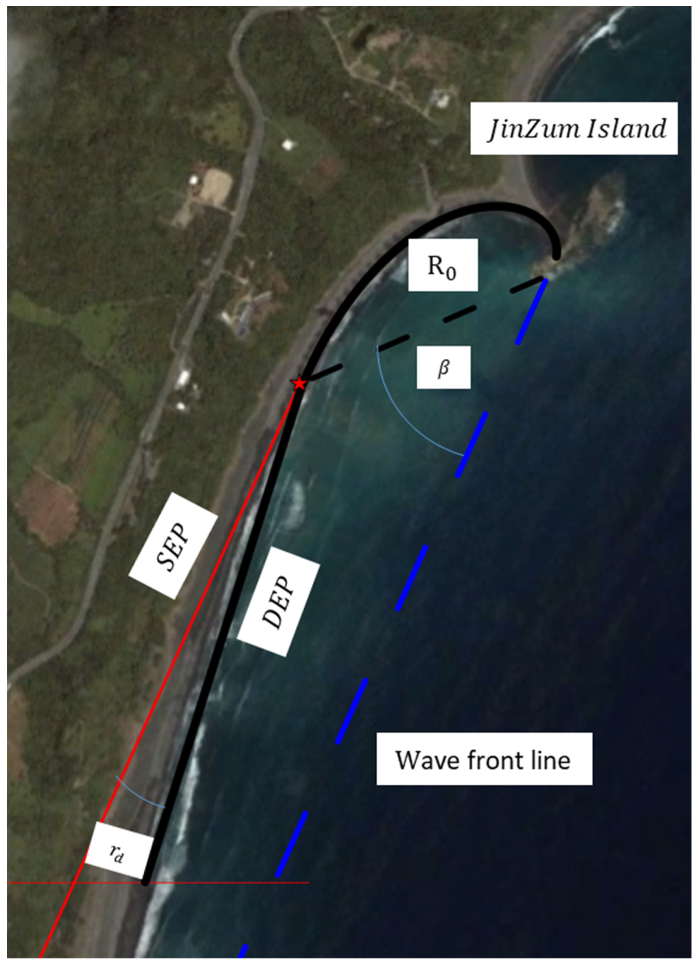
2.2. Dynamic Equilibrium Planform (DEP)

In the numerical experiments in this study, the numerical results of dynamic shoreline planforms of sandy embayed beaches—calculated based on the proposed improved evolution formulation—are compared with the solutions calculated using the dynamic equilibrium planform (DEP) model. Thus, the descriptions of DEP are briefly provided in this section. The DEP model originates in a study on static equilibrium planforms (SEP), which is adopted for the prediction of shoreline planforms in a static equilibrium. The DEP can be derived from the simple and fast second-order polynomial equation of SEP [19,20], and its formulation can be presented as follows:

$$\frac{R}{R_0}=\left(1-\Psi +{\alpha }_{st}\right)+\left(\Psi -2{\alpha }_{st}\right)\left(\frac{\beta }{\theta }\right)+{\alpha }_{st}{\left(\frac{\beta }{\theta }\right)}^2$$

(15)

where $R_0$ denotes the distance between the control point ($P_0$) and the tip of headland, and $\theta$ defines the locations of the shoreline at an angle. $\mathsf{\beta }$ denotes wave obliquity, which is the angle between the incident wave front and the control line. The spatial position of any point along the shoreline can be described by $\left(R,\theta \right)$.$\Psi$ is a function of both the β and $r_d$ angles. More discussions regarding the DEP can be found in Refs. [21,22].

2.3. GenCade [23]

In addition to DEP, the numerical results obtained using the proposed improved evolution formulation are compared with the solutions in GenCade. Therefore, a brief introduction to GenCade is provided. GenCade [23] is a module for calculating the shoreline in SMS using a one-line formulation for shoreline change simulation, as proposed by Ref. [10]. Following many research and development efforts by scholars, the one-line formulation can well take into account factors such as beach nourishment, offshore breakwaters, jetties, and so on, and it has been applied in many practice designs. The one-line formulation [23] in GenCade can be expressed as follows:

$$\frac{\partial \mathrm{y}}{\partial \mathrm{t}}+\frac{1}{(D_B+D_C)}\left(\frac{\partial Q}{\partial x}\right)=0$$

(16)

where $\mathrm{y}$ denotes the shoreline position, and $\mathrm{x}$ denotes the distance alongshore. The longshore sand transport rate $\mathrm{Q}$ is presented in Equation (12). $D_B$ and $D_C$ are the berm elevation and closure depth, respectively. In GenCade, the Cartesian coordinate system and rectangular control volume are adopted; therefore, it is challenging to deal with a high-planform-curvature shoreline. More details regarding GenCade can be found in Ref. [23].

3. Verification of the Proposed Improved Model

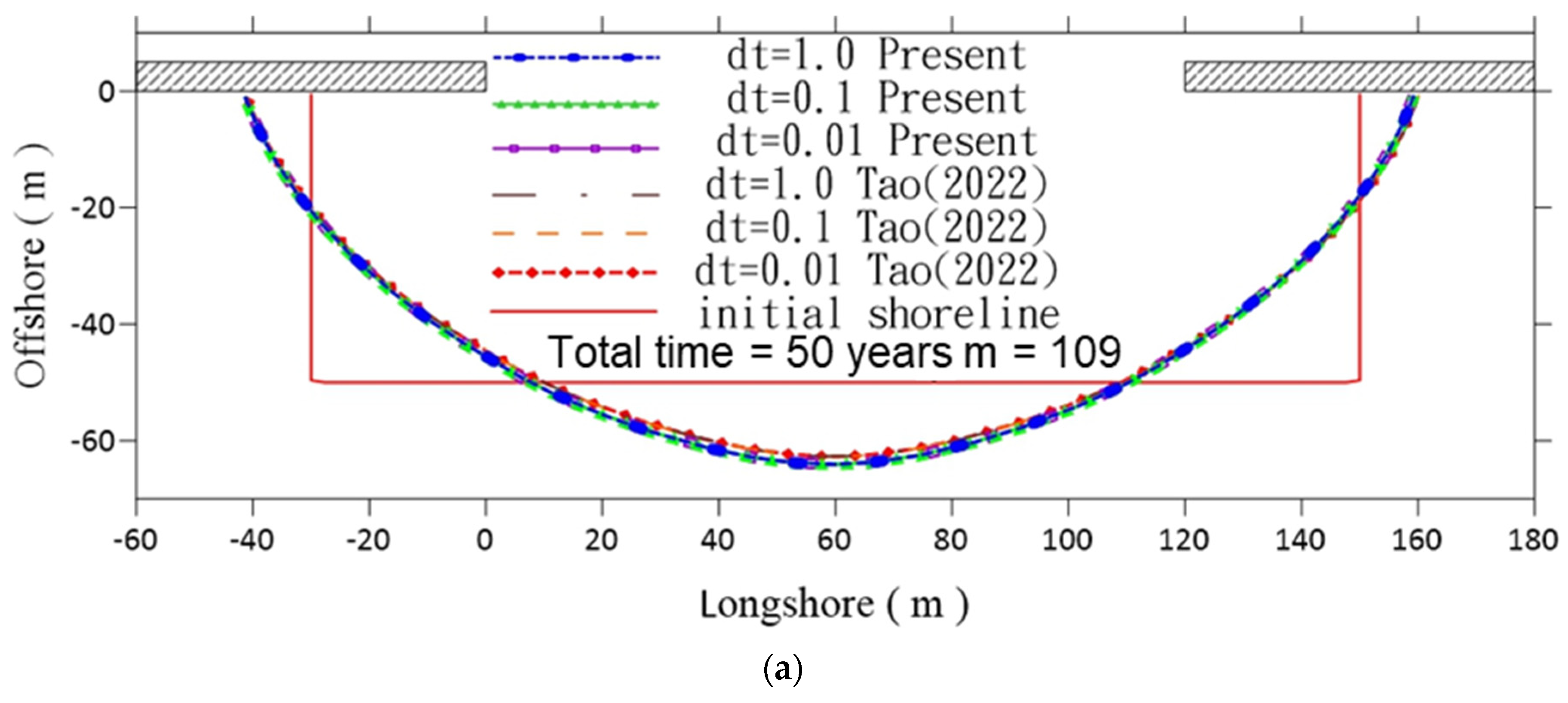
3.1. Example 1: Stability and Consistency

In the first numerical example, we adopt different numbers of shoreline segments $\mathrm{m}$ and different time increments $∆\mathrm{t}$ to verify the consistency and stability of the proposed improved evolution formulation. A schematic diagram of the first example [15] is depicted in Figure 5. There are two breakwaters placed in front of the initial shoreline, and the horizontal distance between the two breakwaters is $G_0$ = 120. In addition, the length of each breakwater is B = 60, and the offshore distance of the breakwaters is S = 50. It can be observed in Figure 5 that the initial shoreline is a composition of three straight lines, which includes two vertical shorelines with an equivalent offshore distance of 50 m and a horizontal shoreline with a length of 180 m.

The origin of the polar coordinate system is placed at the tip of the breakwater on the left, as shown in Figure 5. Once the initial shoreline and initial conditions are imposed, the proposed improved evolution formulation—Equation (11)—can be adopted to accurately and efficiently simulate the dynamic shoreline planform in different time steps. In this numerical test, the wave height of normal incidence is 1 m. Moreover, the EEMSE [24,25] is used to calculate the plane wave fields. The following parameters are used in the numerical experiments: ${\mathrm{K}}_1$ = 0.77, ${\mathrm{K}}_2$ = 0.5, ${\mathrm{D}}_s$ = 10, ρ = 1033, ${\mathsf{\rho }}_s$ = 2650, tanβ = 1/100 and λ = 0.43.

In order to verify the satisfactory consistency and stability of the proposed model, three different numbers of shoreline segments ($\mathrm{m}=109$, $\mathrm{m}=179$, $\mathrm{m}=223$) and three time increments ($∆\mathrm{t}=1$, $∆\mathrm{t}=0.1$, $∆\mathrm{t}=0.01 \mathrm{s}$) are adopted. Based on the numerical experiments, it is found that the shoreline planform will move continuously due to shoreline retreats and shoreline advances. It is noticed in the numerical simulation that the movements of the shoreline planform are negligible for $\mathrm{t}\ge 50 \mathrm{y}\mathrm{e}\mathrm{a}\mathrm{r}\mathrm{s}$; therefore, the profile of the shoreline planform at $\mathrm{t}=50$ years is regarded as a steady-state solution in this case. Hence, the numerical solutions of the shoreline planform in different specific time steps are demonstrated in Figure 6 for $\mathrm{m}=223$ and $∆\mathrm{t}=0.1 \mathrm{s}$. The profiles of the shoreline at $\mathrm{t}=0$, $\mathrm{t}=10 \mathrm{y}\mathrm{e}\mathrm{a}\mathrm{r}\mathrm{s}$, $\mathrm{t}=20 \mathrm{y}\mathrm{e}\mathrm{a}\mathrm{r}\mathrm{s}$, $\mathrm{t}=30 \mathrm{y}\mathrm{e}\mathrm{a}\mathrm{r}\mathrm{s}$, $\mathrm{t}=40 \mathrm{y}\mathrm{e}\mathrm{a}\mathrm{r}\mathrm{s}$ and $\mathrm{t}=50 \mathrm{y}\mathrm{e}\mathrm{a}\mathrm{r}\mathrm{s}$ are exhibited in the figure. The shoreline retreats and shoreline advances are clearly identified in Figure 6, and the numerical results are almost identical to the solutions in our previous study. In addition, it is obvious that the profiles of steady-state shoreline planforms are very distinct from the initial shoreline profiles.

The evolutionary processes of dynamic shoreline movements are depicted in Figure 6, and the numerical accuracy of the proposed model can be verified. Furthermore, the numerical results at $\mathrm{t}=50 \mathrm{y}\mathrm{e}\mathrm{a}\mathrm{r}\mathrm{s}$ when using three different numbers of shoreline segments ($\mathrm{m}=109$, $\mathrm{m}=179$, $\mathrm{m}=223$) are illustrated in Figure 7a–c. The numerical solutions observed in these three figures are almost the same, which can validate the great consistency of the proposed improved evolution formulation. Moreover, in each figure, the numerical results at $\mathrm{t}=50 \mathrm{y}\mathrm{e}\mathrm{a}\mathrm{r}\mathrm{s}$ when using three different time increments ($∆\mathrm{t}=1$, $∆\mathrm{t}=0.1$, $∆\mathrm{t}=0.01 \mathrm{s}$) are exhibited. The satisfactory stability of the proposed model can clearly be verified, since the numerical solutions when using three different time increments in Figure 7a–c are identical to each other. In addition, the numerical results from our previous study are presented in Figure 7a–c, and the good agreement of numerical solutions can verify the accuracy of the proposed numerical scheme. Based on the numerical comparisons in Figure 7a–c, the consistency, stability and accuracy of the proposed improved one-line evolution formulation are apparently validated.

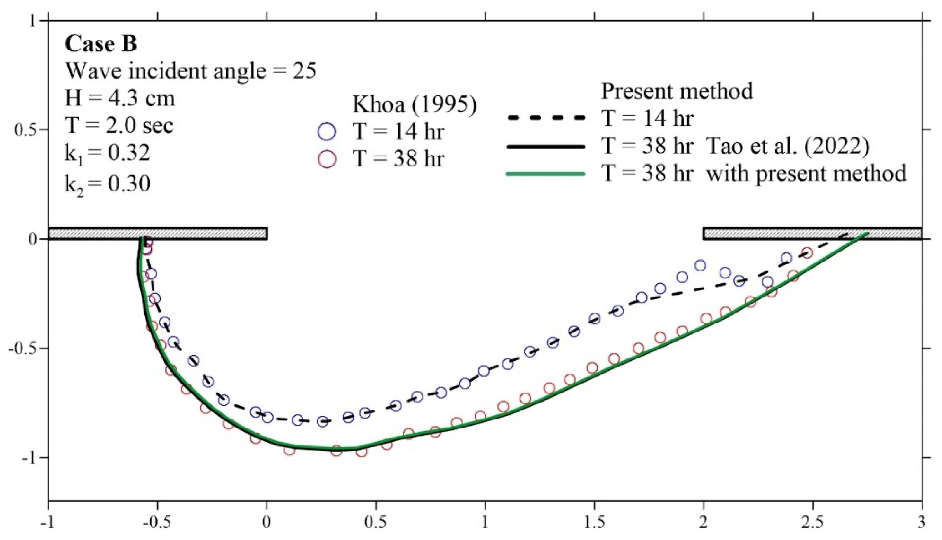
3.2. Example 2: Verification with Experimental Data

For the second example, we adopted the example from Khoa (1995) [25]. A schematic diagram of the second example is depicted in Figure 8. There are two aligned breakwaters placed in front of the initial shoreline. Some parameters are listed in

Table 1. The physical parameters of Example 2.

Parameters	Case B [25]
Incident wave angle (degree)	25
Wave height (cm)	4.3
Wave period (s)	2.0
Water depth at generator (cm)	20
Median grain size, $D_{50}$ (mm)	0.3
Initial beach slope	1.4
Running time (h)	24

. In addition, some conditions and parameters are listed as follows: the incident wave angle is 25$°$; the wave height is 0.43 m; the wave period is 1.3 s; k1 is 0.32; k2 is 0.3; and the simulation time is 24 h. In Figure 8, the initial shoreline for the computer simulation is represented by a dashed line, and the initial shoreline from the experiment results is represented by a blue dot.

The experimental results by [25] and the numerical solutions when using the evolution formulation with/without a correction coefficient are demonstrated in Figure 8. Based on the numerical results in Figure 8, it is obvious that the shoreline planform moved toward the land side due to shoreline retreats. The beginning time is $\mathrm{t}=14 \mathrm{h}$, and the computer simulation will calculate the profile of the embayed beach at $\mathrm{t}=38 \mathrm{h}$. For the solutions at $\mathrm{t}=38 \mathrm{h}$, the experimental data by Khoa (1995) [25] are represented by a red dot; the numerical solution using the evolution formulation without a correction coefficient is represented by a black solid line; and the numerical solution using the improved evolution formulation proposed in this paper is depicted by a green solid line. These three results are very similar to each other, which can apparently verify the accuracy of the proposed improved evolution formulation. On the left-hand side of Figure 8, these three solutions are almost the same. However, on the right-hand side of Figure 8, there are some discrepancies between the solutions. As can be clearly observed, the numerical solution using the proposed formulation is closer to the experimental data than the result using the evolution formulation without a correction coefficient. The comparisons in Figure 8 can clearly show the effectiveness of the proposed improved evolution formulation and the importance of the correction coefficient for the adjustment of inconsistency in the normal direction with the radial direction.

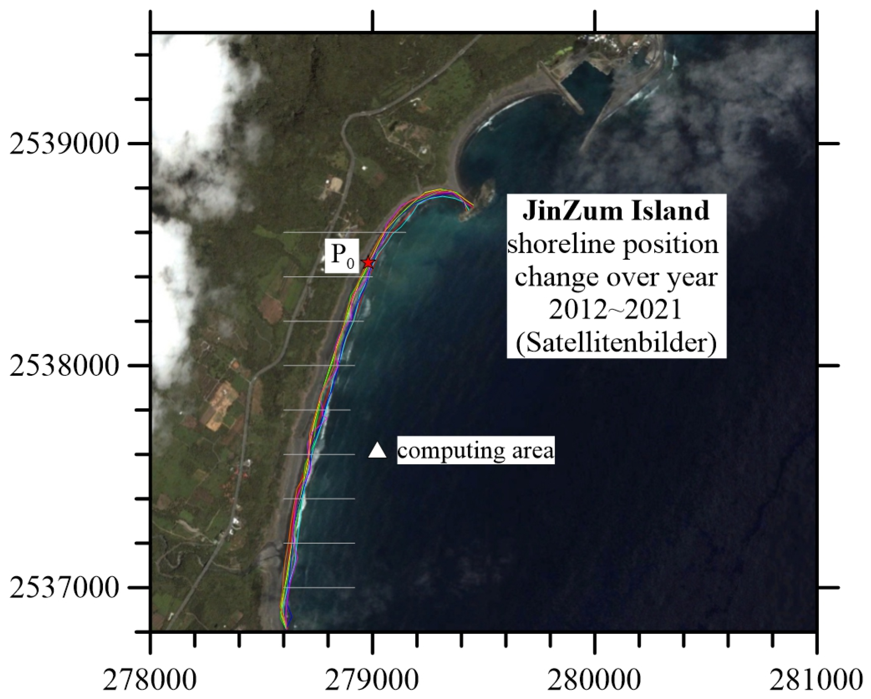
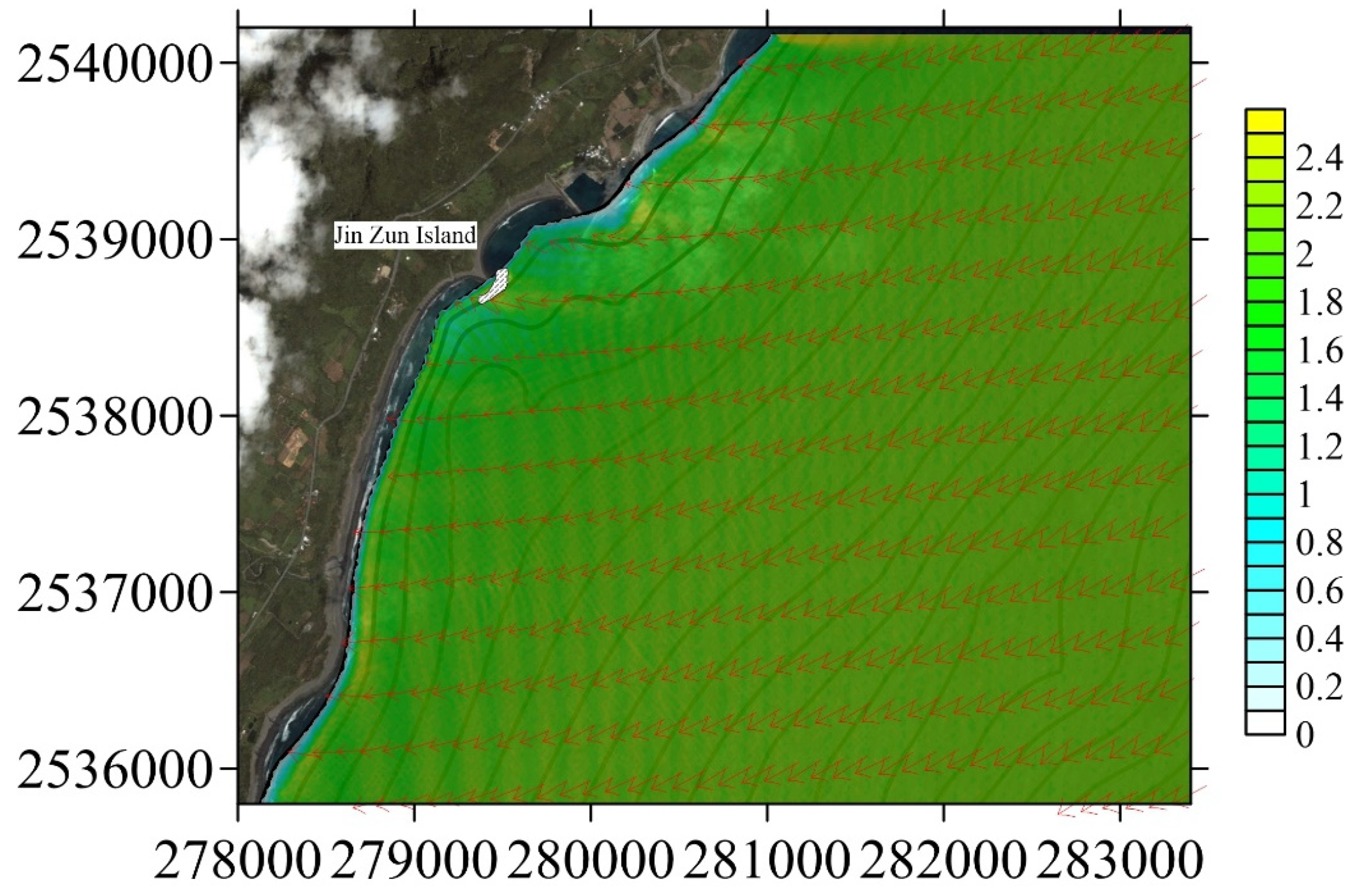
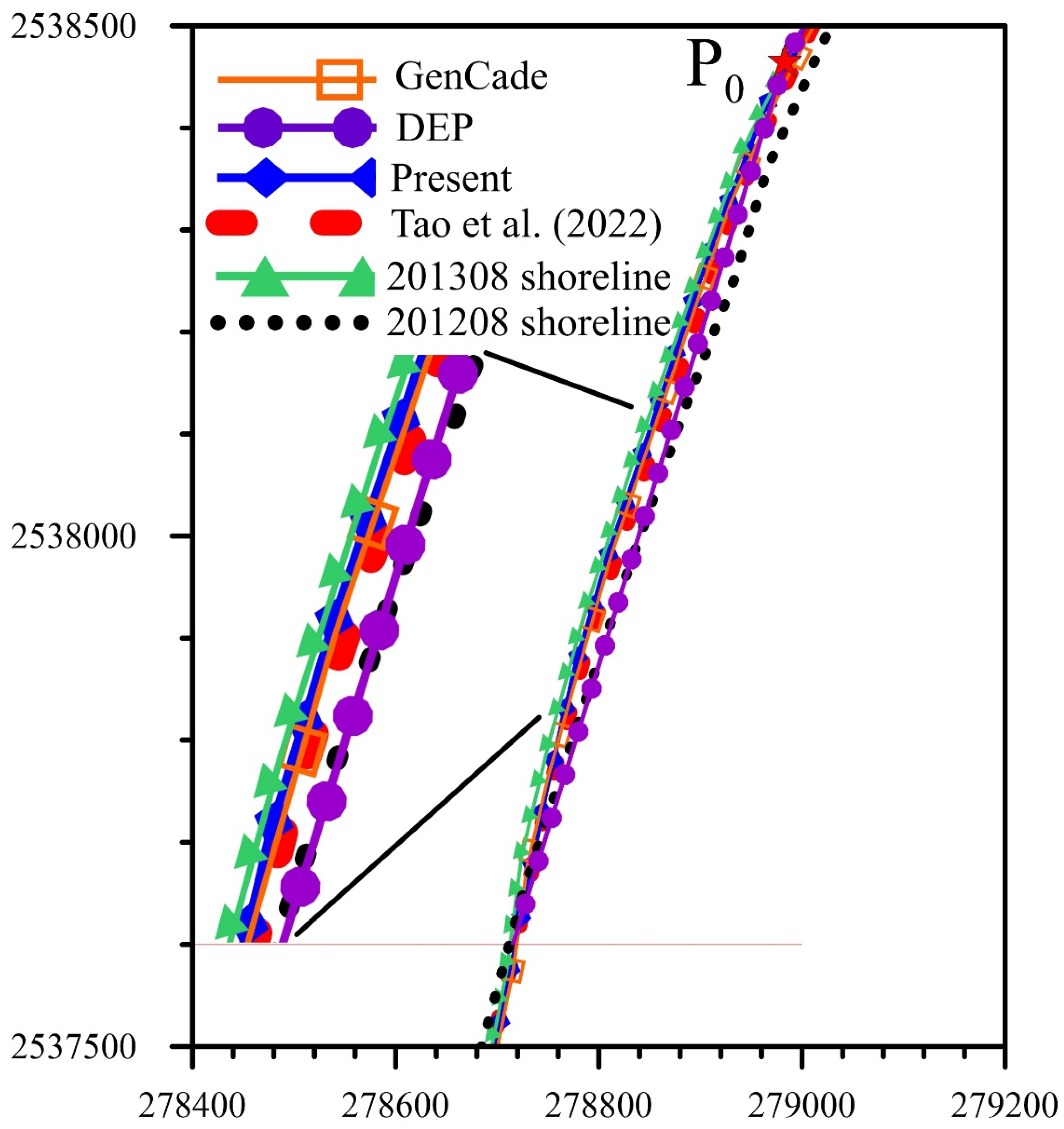
4. Engineering Application

Based on the numerical comparisons in the previous two examples, the merits of the proposed improved evolution formulation are evidently verified. In this section, we are going to adopt a real engineering application along the nature coast. The numerical solutions using the proposed formulation are compared with solutions of the DEP [21,22] and GenCade [23] in a real-world application on the JinZum Island in Taiwan. The JinZum Island is located on the coast of Taitung, Taiwan, and it is the only natural land-connected Island in Taiwan, which is illustrated in Figure 9. On the northern side of JinZum Island, the JinZum Island and the JinZun Fishing Port form two natural and artificial headlands. On the other hand, on the southern side of the JinZum Island, the shoreline planform is an arc-shaped shoreline developed by a single natural headland. In this study, the shoreline along the southern side of the JinZum Island is adopted as the study area.

According to satellite images from 2012 to 2021, it is obvious that the shoreline planform changes from year to year. In order to understand the tendency of shoreline change on JinZum Island, we take the coordinate site y = 2,537,000 m (using TWD 97 as the latitude and longitude coordinate system) as the starting point, with an interval of 200 m, and we set up nine positions to track the change in the shoreline position on the x-axis (yellow line in Figure 9). In Figure 9, the shoreline positions of the nine positions are presented, and it can be found that the shoreline has been retreating over the past nine years.

In Figure 10, it is easily observed that the change in the shoreline demonstrates a negative correlation, with most cross-sections advancing before August 2016 and decreasing thereafter. For a better understanding of annual changes in the shoreline, we used the shoreline data from August 2012 as the baseline and calculated the annual changes relative to it. These calculations are presented in

Table 2. Shoreline change from August 2012 to July 2021.

	Cross-Section	2,538,600	2,538,400	2,538,200	2,538,000	2,537,800	2,537,600	2,537,400	2,537,200
Date
Aug-12		0	0	0	0	0	0	0	0
Jun-13		−15.32	−25.45	−21.62	−13.74	−15.96	−6.79	1.85	−8.59
Aug-13		−33.53	−31.52	−36.50	−30.07	−22.88	1.11	14.79	6.66
Dec-13		−11.92	−12.17	−36.00	−36.27	−4.36	−4.75	2.15	12.08
Jul-14		−13.74	−28.94	−36.24	−26.78	−16.24	3.72	18.26	14.09
Jul-16		11.76	0.31	0.43	3.98	16.12	14.76	24.61	29.54
Jun-17		−16.59	−2.87	−12.42	5.24	9.83	9.58	16.21	10.02
Jan-18		−32.12	−7.04	−17.19	5.75	0.99	−1.46	−3.16	15.67
Dec-18		−49.04	−21.25	−34.72	−8.87	−1.09	1.54	4.42	13.25
Apr-21		−56.51	−62.86	−72.43	−40.74	−28.78	−16.10	3.70	−14.04
Jul-21		−37.63	−37.48	−39.46	−14.68	−25.85	4.16	−8.15	−8.93
Shoreline change rate (m/year)		−4.02	−2.45	−3.03	−0.03	−0.71	−0.025	−0.70	−0.4

. Shoreline change is measured from August 2012 to July 2021, with the shoreline change rate ranging from −4.02 m per year to −0.025 m per year, while the distance increases from the headland to y = 2,537,600. Beyond y = 2,537,600, the shoreline change rate decreases to −0.7 m per year and −0.4 m per year. Based on the above information, the position at y = 2,537,600 should be the end of sediment longshore transport, located downcoast of the JinZum Island. Therefore, we take y = 2,538,800 as the starting point for the calculation area, and y = 2,537,600—where the minimum shoreline change rate occurs—is considered as the endpoint of the calculation area. The length of the shoreline is approximately 1300 m.

Before commencing the computer simulation, the wave data in the considered region over the past years from 2012 to 2021 were collected from the Central Weather Bureau of Taiwan. These data are freely available for public use on a website and are tabulated in

Table 3. Model conditions and wave data near JinZum Island.

	DEP [20,21]	GenCade [22]	Present/[14]
Wave data from buoy
Height	2.1 m
Period	8.2 s
Direction	$59°$
Model parameters
${\mathit{r}}_{\mathit{d}}$	$8°$	-
$\mathsf{\beta }$	$43°$	-
${\mathit{R}}_0$ (m)	430	-
m	-	450	223
$∆\mathbf{t}$ (s)	-	0.01
Cell size (m)		5
${\mathit{k}}_1$	-	0.77
${\mathit{k}}_2$	-	0.38
Simulation time (day)	-	365
Initial wave condition
Height	1.5 m
Period	8.2 s
Direction	$114°$

. Based on the statistics of wave buoy, the wave height is 2.1 m; the wave period is 8.2 s; and the wave direction is $59°$. In this study, we used buoy data as the initial wave condition in EEMSE to calculate the distribution of the wave field in the nearshore area in JinZum Island, and the wave data in the headland were taken as the incident wave direction used in subsequent models. Accordingly, the wave field results from EEMSE are shown in Figure 11. In the figure, the wave height decreased from 2.1 m to 1.5 m, and the direction of water wave changed from $59°$ to $114°$ in the headland of JinZum Island.

Once the wave fields in the nearshore area are obtained, we have to define some parameters in the DEP, GenCade and the proposed model. In the DEP, the length from the headland cap to the control point ($R_0$) is defined as 430 m; therefore, the control point $P_0$ can be determined and located. In addition, $\mathsf{\beta }$ is $43°$, and $r_d$—the angle between the SEP and DEP—is $8°$. The above definitions and parameters in the DEP are depicted in Figure 12. In addition to the DEP, GenCade and the proposed formulation are adopted to simulate the same problem in JinZum Island. Both GenCade and the proposed formulation belong to the one-line model; therefore, they require the same parameters, such as $∆\mathrm{t}=0.01 \mathrm{s}$, $K_1=0.77$, $K_2=0.38$. In this example, the simulation time in GenCade and the proposed formulation is defined as $0\le \mathrm{t}\le 365 \mathrm{d}\mathrm{a}\mathrm{y}\mathrm{s}$ (from 2012 to 2013). Although GenCade and the proposed formulation are one-line models, GenCade uses the Cartesian coordinate system, and the proposed formulation adopts the polar coordinate system. Thus, the schemes for spatial discretizations of these two one-line models are different from each other. For the proposed improved formulation, $\mathrm{m}=223$ is used to define the number of adjacent shoreline segments. However, in GenCade, we use $∆\mathrm{x}=5 \mathrm{m}$ to define the length of every shoreline segment.

The shoreline positions from August 2012 are adopted as the initial condition for numerical simulation. The initial shoreline planform in August 2012, the realistic shoreline planform in August 2013 and the numerical results of DEP, GenCade and the proposed improved formulation are demonstrated in Figure 13. The good agreement of solutions in Figure 13 reveals that DEP, GenCade, Tao et al. (2022) [14,20,21,22] and the proposed improved formulation can all accurately simulate the dynamic movement of a shoreline planform in a sandy embayed beach. The numerical results are very similar to each other both in the hooked zone and the unhooked zone. Based on the solutions in Figure 13, it is evident that shoreline retreat occurred from 2012 to 2013 under wave interaction. In the comparisons in Figure 13, we can carefully observe a slight discrepancy between these solutions. Therefore, the shoreline comparisons in the northern part of the control point are presented in Figure 13, and the shoreline planform solutions in the southern part of the control point are displayed in Figure 13.

The shoreline planform comparisons in the northern part of the control point are depicted in Figure 14. Although the numerical solutions are very similar to the realistic shoreline planform obtained from satellite images, the numerical solutions of DEP from the previous study and the proposed improved one-line formulation are closer to the practical shoreline planform than GenCade. GenCade—a one-line model—adopts the Cartesian coordinate system to describe the entire shoreline planform; therefore, it is complicated to apply GenCade when dealing with high-planform-curvature shorelines, such as the shoreline in the hooked zone. In the shoreline located in the northern part of the control point, the performances of DEP and the proposed formulation are superior to GenCade.

The numerical comparisons for the shoreline planform in the southern coastal area of the control point are depicted in Figure 15. In addition to the obvious shoreline retreats, the shoreline planforms in 2012 and 2013 are very similar to a straight line. In the southern coastal area of the control point, there are no artificial or natural structures in the unhooked zone; therefore, it is reasonable to expect a straight shoreline. Since there is no high-planform-curvature shoreline, the Cartesian-coordinate-based GenCade can be expected to obtain a better solution in comparison with the other two polar-coordinate-based schemes, which include the DEP, a previous study and the proposed formulation. In Figure 15, the numerical solutions of GenCade, the previous study and the proposed formulation are closer to the practical shoreline in August 2013 than the results from DEP. Comparing the previous study and the present method, although there is higher consistency within the hooked zone, the results in the unhooked zone demonstrate that the method proposed in this study effectively corrects volume deformation and achieves higher precision than the previous method. Furthermore, it is surprising to find that the solution of the proposed formulation is closer to the practical shoreline than GenCade. Based on the numerical comparisons in Figure 14 and Figure 15, it can be verified based on a realistic engineering application that the proposed improved one-line evolution formulation can be adopted to accurately and efficiently simulate the dynamic movements of sandy embayed beaches. In addition, with the help of the correction coefficient, the proposed formulation can acquire accurate shoreline planforms both in the hooked and the unhooked zones.

5. Conclusions

In this paper, an improved one-line evolution formulation for dynamic shoreline planforms of sandy embayed beaches is proposed and examined. In order to eliminate the possible weakness of the one-line model, based on the Cartesian coordinate system or the hybrid coordinate system, the polar coordinate system is adopted in this paper to derive the evolution formulation. In addition, the rectangular control volume is used to avoid the quadratic term in the evolution formulation. Since the rectangular control volume is adopted, the straight shoreline segment is assumed to move along the normal direction. However, if the polar coordinate system is adopted, the movements of the shoreline segment will be found along the radial direction of the polar coordinate system. In order to overcome the misaligned directions of these two vectors, a correction coefficient is derived and forms the proposed improved one-line evolution formulation. The distance of shoreline retreats or shoreline advances along the normal direction is adjusted to the radial direction, so that the improved one-line evolution formulation derived can accurately and efficiently calculate the dynamic movements of every shoreline segment.

In order to verify the merits of the proposed improved evolution formulation, three examples are provided in this paper. In the first example, the stability and consistency of the proposed model are evidently validated using different numbers of shoreline segments and different time increments. In the second example, the numerical results are closer to experimental data than the other solutions obtained using the evolution formulation without a correction coefficient. The numerical comparisons in the second example demonstrate the effectiveness of the correction coefficient and the proposed evolution formulation. Moreover, the shoreline retreats in the southern part of the JinZum Island are adopted as the third example. In a practical engineering application, the numerical models of DEP, the previous study and GenCade are used in addition to the proposed improved model. Based on the numerical comparisons in the third example, it is verified that the proposed improved one-line model outperforms the DEP and GenCade both in the hooked zone and the unhooked zone; the model shows that a correction coefficient could improve the one-line evolution formulation for dynamic shoreline planforms in the down coast. In future, cross-shore sediment transport will be included in the proposed improved evolution formulation for dynamic shoreline planforms of embayed beaches.

References

1. Safari, M.D. A short review of submerged breakwaters. In Proceedings of the MATEC Web of Conferences, Malang, Indonesia, 30–31 August 2018; p. 01005. [Google Scholar]
2. Skaggs, L.L.; McDonald, F.L. National Economic Development Procedures Manual. Coastal Storm Damage and Erosion; Army Engineer Inst for Water Resources Alexandria Va (USA): Alexandria, VA, USA, 1991. [Google Scholar]
3. Lin, T.; Van Onselen, V.; Vo, L. Coastal erosion in Vietnam: Case studies and implication for integrated coastal zone management in the Vietnamese south-central coastline. In Proceedings of the IOP Conference Series: Earth and Environmental Science, Surakarta, Indonesia, 24–25 August 2021; p. 012009. [Google Scholar]
4. Özölçer, İ.H.; Kömürcü, M.İ.; Birben, A.R.; Yüksek, Ö.; Karasu, S. Effects of T-shape groin parameters on beach accretion. Ocean Eng. 2006, 33, 382–403. [Google Scholar] [CrossRef]
5. Liang, T.-Y.; Chang, C.-H.; Hsiao, S.-C.; Huang, W.-P.; Chang, T.-Y.; Guo, W.-D.; Liu, C.-H.; Ho, J.-Y.; Chen, W.-B. On-Site Investigations of Coastal Erosion and Accretion for the Northeast of Taiwan. J. Mar. Sci. Eng. 2022, 10, 282. [Google Scholar] [CrossRef]
6. Putro, A.H.S.; Lee, J.L. Analysis of longshore drift patterns on the littoral system of nusa dua beach in bali, indonesia. J. Mar. Sci. Eng. 2020, 8, 749. [Google Scholar] [CrossRef]
7. Hsu, J.R.C.; Evans, C. Parabolic Bay Shapes and Applications. Proc. Inst. Civ. Eng. 1989, 87, 557–570. [Google Scholar] [CrossRef]
8. Yasso, W.E. Plan geometry of headland-bay beaches. J. Geol. 1965, 73, 702–714. [Google Scholar] [CrossRef]
9. Hsu, J.R.; Silvester, R.; Xia, Y.-M. Applications of headland control. J. Waterw. Port Coast. Ocean Eng. 1989, 115, 299–310. [Google Scholar] [CrossRef]
10. Pelnard-Considère, R. Essai de theorie de l’evolution des formes de rivage en plages de sable et de galets. Journ. Hydraul. 1957, 4, 289–298. [Google Scholar]
11. Francone, A.; Simmonds, D.J. Assessing the Reliability of a New One-Line Model for Predicting Shoreline Evolution with Impoundment Field Experiment Data. J. Mar. Sci. Eng. 2023, 11, 1037. [Google Scholar] [CrossRef]
12. Hanson, H. GENESIS: A generalized shoreline change numerical model. J. Coast. Res. 1989, 5, 1–27. [Google Scholar]
13. Weesakul, S.; Tasaduak, S. Experimental investigation on dynamic equilibrium bay shape. Coast. Eng. 2012, 2, 1–13. [Google Scholar] [CrossRef]
14. Tao, H.-C.; Hsu, T.-W.; Fan, C.-M. Developments of Dynamic Shoreline Planform of Crenulate-Shaped Bay by a Novel Evolution Formulation. Water 2022, 14, 3504. [Google Scholar] [CrossRef]
15. Ozasa, H.; Brampton, A. Mathematical modelling of beaches backed by seawalls. Coast. Eng. 1980, 4, 47–63. [Google Scholar] [CrossRef]
16. Kraus, N.C.; Harikai, S. Numerical model of the shoreline change at Oarai Beach. Coast. Eng. 1983, 7, 1–28. [Google Scholar] [CrossRef]
17. Weesakul, S.; Rasmeemasmuang, T.; Tasaduak, S.; Thaicharoen, C. Numerical modeling of crenulate bay shapes. Coast. Eng. 2010, 57, 184–193. [Google Scholar] [CrossRef]
18. Tan, S.-K.; Chiew, Y.-M. Analysis of bayed beaches in static equilibrium. J. Waterw. Port Coast. Ocean Eng. 1994, 120, 145–153. [Google Scholar] [CrossRef]
19. Tan, S.; Chiew, Y. Bayed beaches in dynamic equilibrium. Adv. Hydro-Sci. Eng. I 1993, 1737–1742. [Google Scholar]
20. Elshinnawy, A.I.; Medina, R.; González, M. Dynamic equilibrium planform of embayed beaches: Part 1. A new model and its verification. Coast. Eng. 2018, 135, 112–122. [Google Scholar] [CrossRef]
21. Elshinnawy, A.I.; Medina, R.; González, M. Dynamic equilibrium planform of embayed beaches: Part 2. Design procedure and engineering applications. Coast. Eng. 2018, 135, 123–137. [Google Scholar] [CrossRef]
22. Frey, A.E.; Connell, K.J.; Hanson, H.; Larson, M.; Thomas, R.C.; Munger, S.; Zundel, A. GenCade Version 1 Model Theory and User’s Guide; U.S. Army Engineer Research and Development Center, Coastal and Hydraulics Laboratory: Vicksburg, MS, USA, 2012. [Google Scholar]
23. Hsu, T.-W.; Wen, C.-C. A parabolic equation extended to account for rapidly varying topography. Ocean Eng. 2001, 28, 1479–1498. [Google Scholar] [CrossRef]
24. Hsu, T.-W.; Wen, C.-C. On radiation boundary conditions and wave transformation across the surf zone. China Ocean Eng. 2001, 15, 395–406. [Google Scholar]
25. Khoa, V. Experimentation on Bayed Beaches between Headlands for Small Wave Angle. Master’s Thesis, Asian Institute of Technology, Bangkok, Thailand, 1995. Volume 10. 90p. [Google Scholar]
Figure 1. A schematic diagram of the shoreline planform of crenulate-shaped bay.
Water 16 00774 g001
Figure 2. The control volume between two sequential time steps.
Water 16 00774 g002
Figure 3. The control volume defined in this study and its dimension.
Water 16 00774 g003
Figure 4. A schematic diagram of the different angles adopted in this study.
Water 16 00774 g004
Figure 5. A schematic of the numerical example for verification of consistency and stability.
Water 16 00774 g005
Figure 6. Numerical results in different specific time frames when using the proposed improved one-line model ( m = 223 , t = 0.1 ).
Water 16 00774 g006
Figure 7. Numerical results and comparisons with Ref. [14] when using different ∆t for (a) m = 109, (b) m = 179 and (c) m = 223.
Water 16 00774 g007aWater 16 00774 g007b
Figure 8. Numerical results and comparison of Example 2 [14,25].
Water 16 00774 g008
Figure 9. Changes in the shoreline near JinZum Island in the past years (2012~2021, TWD 97).
Water 16 00774 g009
Figure 10. The spatial position of the nine shoreline positions over the past years.
Water 16 00774 g010
Figure 11. Numerical solution from EEMSE for the wave field in nearshore area.
Water 16 00774 g011
Figure 12. Geometric definitions of the DEP in JinZum Island.
Water 16 00774 g012
Figure 13. Numerical results of DEP, GenCade, Tao et al. (2022) [14] and the present formulation for the shoreline planform in August 2013.
Water 16 00774 g013
Figure 14. Comparisons of numerical solutions along the shoreline portion between the control point and the JinZum Island [14].
Water 16 00774 g014
Figure 15. Numerical comparisons for the shoreline planform in the southern coastal area of the control point [14].
Water 16 00774 g015