Abstract
Fish protection is a priority in regions with ongoing and planned development of hydropower production, like the Mekong River system. The evaluation of the effects of turbine passage on the survival of migratory fish is a primary task for informing hydropower plant operators and authorities about the environmental performance of plant operations. The present work characterizes low pressures and collision rates through the Kaplan-type runners of the Xayaburi hydropower station. Both an experimental method based on the deployment of Sensor Fish and a numerical strategy based on flow and passage simulations were implemented on the analysis of two release elevations at one operating point. Nadir pressures and pressure drops through the runner were very sensitive to release elevation, but collision rates on the runner were not. The latter showed a frequency of occurrence of 8.2–9.3%. Measured magnitudes validated the corresponding simulation outcomes in regard to the averaged magnitudes as well as to the variability. Central to this study is that simulations were conducted based on current industry practices for designing turbines. Therefore, the reported agreement helps turbine engineers gain certainty about the prediction power of flow and trajectory simulations for fish passage assessments. This can accelerate the development of environmentally enhanced technology with minimum impact on natural resources.
1. Introduction
Hydropower constitutes 55% of renewable electricity generation worldwide [1], and the current demands for decarbonizing the economy have created a positive outlook for the sector. This includes expanding production from existing dams as well as constructing and planning of new ones by 2030 [2]. Despite this favorable growth, there remain legitimate concerns about potential negative impacts on the health of aquatic systems. One concern centers around the disruptions of upstream and downstream fish migration, including mechanisms that may contribute to injury and mortality [3]. Turbine passage, in particular, has been listed as one of the main challenges to be resolved to increase hydropower sustainability and public acceptance [4]. In response to such a challenge, some projects around the world have pursued novel geometric designs and operational strategies for enhancing turbine passage survivability for fish [5]. This effort has led to the development of strategies for assessing the biological performance of turbines, which consists of quantifying risks of injury and mortality related to turbine passage using modeling approaches, experimenting in research laboratories, and conducting field tests with sensors and live fish. The most widely accepted method is the in situ measurement of “direct survival rates” by purposely entraining live fish into turbine flows and recapturing them after passage for biological inspection [6,7]. Looking at the steps for searching for sustainable turbine designs (Figure 1), live fish testing seeks to correlate the design/operating condition (step i) in question to the biological outcome (step iv). Decades of testing turbines with live fish shed light on the intermediate factors driving survival rates, namely the occurrence and intensity of key hydraulic stressors (step ii in Figure 1) and the exposure of passing fish to such hydraulic stressors (step iii). The redefinition of the biological performance in terms of steps (ii) and (iii) becomes relevant for hydropower operators and turbine designers, who can then steer new turbine designs and operational strategies towards an environmentally relevant target in a more effective manner.
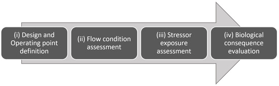
Figure 1.
A representation of the steps towards sustainable turbine design.
Much of the international literature pertaining to fish passage and survival relates to northern hemisphere species, especially salmonids [8,9,10]. There are relatively few data available on tropical and neotropical rivers. These are of particular concern, as many species in these zones have complex life history strategies and are hugely biodiverse. Thus, turbine design criteria in these systems needs to consider eggs, larvae, juveniles, sub-adults, and adults across a range of species with very complex monsoonal hydrology. One such region is the Mekong River of Southeast Asia. Relatively few data are available on sustainable turbine design for the many species that inhabit this important system.
For instance, some studies have investigated the biological effect of shear stress on the bodily injury of fish species of the Mekong River. Baumgartner et al. [11] set up laboratory simulations of exposure of silver shark (Balantiocheilos melanopterus) to high shear flow conditions in a hydraulic flume and reported injuries such as exophthalmia and spinal injuries at extremely high exposure rates (1296 s−1). Another study [12] observed bruises and frays for iridescent shark (Pangasianodon hypophthalmus) at strain rates greater than 1000 s−1) and gill damage in blue gourami (Trichopodus trichopterus) at rates of 688 s−1. It is unknown if these shear stress levels materialize in turbine passage and, if they do, the frequency that fish are exposed to these high shear levels is likewise unknown. No equivalent information is known about the effects of pressure and collisions on local fish, and field measurements with Sensor Fish offer a possibility to characterize the magnitudes of fish-relevant hydraulic stressors.
Quantifying the magnitudes of the key hydraulic stressors in the Kaplan-type turbines of the Xayaburi hydropower plant (HPP) is the primary goal of the work presented herein. The Xayaburi HPP is the first mainstem dam to have been constructed in the Mekong River. This research seeks to understand the hydraulic parameters of the hydropower system as they relate to passage of a multi-species community. This was accomplished by, first, onsite measurements with Sensor Fish (SF, Section 3.2) and, second, simulations of turbine flow and passage with industry-oriented modeling practices (Section 4.2). Previous studies have conducted either SF-based field assessments or simulation-based desktop evaluations; to the best of our knowledge, this is the first study to implement both techniques simultaneously on the same case. Such findings could be of scientific value for both the HPP operator and turbine engineers.
The first pillar of the present work consisted of the onsite deployments of Sensor Fish (SF). The SF was developed at the Pacific Northwest National Laboratory (Richland, WA, USA, [13,14]), is licensed to Advanced Telemetry Systems, Inc (Isanti, MN, USA), and collects hydraulic information about what fish may most likely experience during passage through turbines in operation. The Sensor Fish has been deployed at various hydropower stations around the world. At the Wanapum dam in the Columbia River, SF measurements through two distinct large Kaplan-type turbines—one old and one new—demonstrated lower collision rates and greater passage pressure conditions for the new turbine than for the old design [15]. Early SF studies (e.g., see Dauble et al. [16]) established experimental practices that became the backbone of subsequent field tests of this kind, such as the definition of discharge, head and release depth as predictor (treatment) variables, and the frequency of collisions, low pressures, and turbulence levels as experimental outcomes. At the Ice Harbor HPP equipped with large Kaplan units, Martinez et al. [17] reported lower pressure conditions with higher discharge, the lowest SF rotation rates, and the highest frequency of collisions at peak efficiency (mid-level discharge). In Francis-type turbines, SF measurements showed much lower pressures during passage and a greater occurrence of collisions on blades in comparison to Kaplan units [18]. SF deployments through a siphon-type turbine revealed the lowest pressure conditions and the highest collision frequency among all turbine types that had been tested at that time [19]. In testing the hypothesis that low-head turbines offer safer fish passage, Boys et al. [20] reported that unfavorable magnitudes of hydraulic stressors to fish are present in a low-head Kaplan runner (high frequency occurrence of sub-atmospheric pressures) and in an Archimedes screw (high frequency of collisions). These field studies served as a reference for the field study reported herein.
The second pillar of the present work involves numerical simulations of fish passages through the Xayaburi Kaplan-type turbine. The use of flow simulations for developing new turbines, as well as for examining flow phenomena posterior to design, is a long-standing practice in industry [21,22]. Using flow simulations for fish passage analyses was first conceived by Ventikos et al. [23], who proposed a Lagrangian approach for calculating the likely pathways of fish swimming through 3D simulated fields of pressure, velocity, and turbulence in turbine flows related to computational fluid modeling. With this seminal work as a basis, further developments concentrated on two fronts: (i) increasing the accuracy of the fish-focused hydraulic predictions and (ii) enabling the efficient investigation of various scenarios via computer software. Both fronts contribute to the development of improved turbine designs. A major development is the Biological Performance Assessment toolkit (BioPA, Pacific Northwest National Laboratory, Richland, WA, USA [24,25]), which takes a 3D flow simulation, trajectory starts, and other site settings to calculate magnitudes of fish-relevant hydraulic stressors, as well as an index value (score) that characterizes the overall risks of mortal injury. This score serves as an indicator when comparing various operating conditions, distinctive turbine designs, or specific entrainment locations of passing fish. Simulation-based assessments of fish passage for different turbine types can be found in the work of Müller et al. [26] and Zhu et al. [27], who investigated the hydraulic parameters affecting fish survival through Francis-type turbines; Klopries and Schüttrumpf [28], who investigated the passage of European eels (Anguilla anguilla) through a bulb-type turbine; and Singh et al. [29], who examined passage conditions through a very large Kaplan turbine by representing fish as Lagrangian particles. Simulation-based assessments have not yet been satisfactorily validated with SF field measurements. The novelty of the present work consists of deploying flow simulation technology for examining fish passage through a large Kaplan-type turbine in a way that it provides meaningful information to design biological experiments on local species of the Mekong River. The greatest challenge to overcome herein is to validate the computer-based assessment with field data collected at the HPP, and this is only possible by implementing both techniques—simulation- and SF-based assessments—on the same case.
The goal of the present work is to:
- Characterize hydraulic passage conditions in the very large Kaplan turbine of the Xayaburi HPP;
- Test the hypothesis that corresponding flow and passage simulations reproduce fish-relevant hydraulics satisfactorily. It is important to implement simulation protocols amenable to industry practices.
2. Investigated Hydraulic Stressors That Influence Fish Passage Survival
When fish pass rotating turbines, they are exposed to a number of hydraulic stressors, leading to mortal injury. Such hydraulic stressors have been broadly discussed and summarized ([7,30]), but the extent to which they affect fish survival continues to be an active subject of research [12]. The nearly simultaneous occurrence of stressors during passage adds a greater degree of difficulty to the challenge of linking hydraulic conditions to consequential survivability. For turbine engineers, research summaries have recommended a list of a turbine’s geometric features that may enhance fish passage conditions [31,32], and engineering teams in industry try to influence two main stressors: the rate and intensity of collisions on blades and the occurrence of low pressure conditions. These two turbine passage stressors are not the only ones that occur during passage but are the most extensively documented. Biological evaluations of injury types and extent resulting from pressure and collisions in an accurate and systematic manner have been conducted [33,34], but linking a specific injury type to one specific stressor is not yet entirely clear, as fish are often exposed to stressors in sequence, and multiple stressors act upon fish simultaneously [35]. We provided herein an overview of the latest knowledge about the link between the investigated hydraulic stressors in this study and the injury types they cause.
2.1. Collision on Blades
Fish maycollide with solid surfaces during passage through turbines. Although these collisions may occur on any wall, collisions on rotating runner blades are considered the most lethal for passing fish. Pracheil et al. [7] suggested that the mechanical wounding caused by blade strikes may manifest in the form of bruising, descaling, laceration, hemorrhage, amputation, and decapitation. It is noteworthy that collisions on blades appear to lead to externally visible injuries [33]. Regarding quantification, the effect of blade strike on fish survival is a two-step calculation that involves: (i) the likelihood that a collision takes place () and (ii) the likelihood that the strike leads to mortal injury once it takes place. This study focuses on the assessment of component (i), that is , based on Sensor Fish measurements and flow simulations.
From Sensor Fish measurements, the likelihood of collision is calculated as the relative frequency of collision occurrence. Collected SF data showed sharp spikes in acceleration measurements whenever SF experienced any contact on a wall. However, not all contacts are collisions; the timing and magnitude of such spikes are post-processed to determine, first, whether the acceleration spike resulted from a collision or not, and second, if such collision took place within the runner [13]. Therefore, the frequency of collision, Equation (1), results from dividing the number of SF that exhibited at least one collision in the runner region () by the total number of deployed SF (). More details about SF signals and data post-processing are provided in Section 3.4 and Section 5.2, respectively.
From flow and passage simulations, passage conditions are calculated based on the simulated trajectory as the SF approaches the leading edge of the blade (further details are provided in Section 4.3). The instant of runner passage is represented in Figure 2. Information at this instant is extracted from the 3D flow field to calculate the likelihood that a collision occurs, Equation (2), based on passage velocities ( and , in m/s), passage angle (), fish length (L, in m), and thickness of the leading edge (T, in m). The number of blades (N) plays a role in the magnitude of , as well as the rotational speed of the runner (n, revolutions per second).
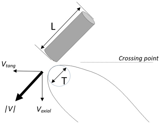
Figure 2.
A schematic representation of the SF passage at the moment that it approaches the leading edge of the runner blade.
2.2. Nadir Pressure
Fish experience strong pressure variations as they pass turbines in operation (Figure 3). Typically, they approach the turbine at nearly hydrostatic pressure levels that solely depend on the swimming depth. If entrained into the turbine flow, fish experience a gradual mild pressure increase as they enter the distributor (the maximum value is usually found near the distributor entrance), followed by a sudden drop () as fish pass through the runner and encounter a minimum pressure value (also known as “nadir pressure”, ). Next, pressure levels recover at the draft tube until they again reach a hydrostatic pressure behavior at the draft tube outlet. Fish can adapt to pressure changes, but they do so naturally at a pace much slower than the rate of pressure change typically encountered during passage. These high pressure change rates may cause stomach eversion, exophthalmia (eye pop), swim bladder rupture, embolism, and hemorrhage [36]. Contrary to the injury types caused by collisions, low pressures appear to lead to internal injuries that may be better identified and evaluated via X-rays [34]. Brown et al. [9] suggested that mortal injuries associated with decompression through turbines depend on the ratio of the pressure at which fish were acclimated immediately before the passage event (acclimation pressure) to nadir pressure. Therefore, we characterized pressure conditions with and a proxy value for the acclimation pressure because the actual acclimation pressure cannot be known unless monitoring data of approaching fish are available. In conformity with previous studies [17,37], this work determined absolute pressure at the distributor entry () to calculate a proxy pressure drop as follows:
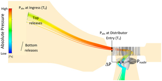
Figure 3.
Absolute pressure variation during passage through the Kaplan turbine of Xayaburi HPP and SF release locations.
From Sensor Fish measurements, data post-processing yielded both the and values, with which can be determined (see Section 3.4 and Section 5.2).
From flow and passage simulations, the time series of absolute pressure is likewise extracted from each simulated fish pathway, which allowed us to extract , , and from all simulated trajectories.
All pressure values were normalized (, in Equation (4)) with respect to a minimum () and maximum () reference pressure, which were the same for all values reported and discussed in this work:
3. Sensor Fish Measurements
3.1. Site, Turbine, and Operational Information
The Xayaburi HPP is located in the Lower Mekong River section of Lao PDR, with geographic coordinates 19° 14′ 35′′ N, 101° 49′ 06′′ E. The HPP is owned by the company Xayaburi Power Company Limited (XPCL) and started commercial operation in October of 2019. The spillway consists of seven radial gates and four low-level outlets with a capacity of 47,500 m3/s. The reservoir capacity is 726 million m3, from a catchment area of 272,000 km2 (Figure 4).
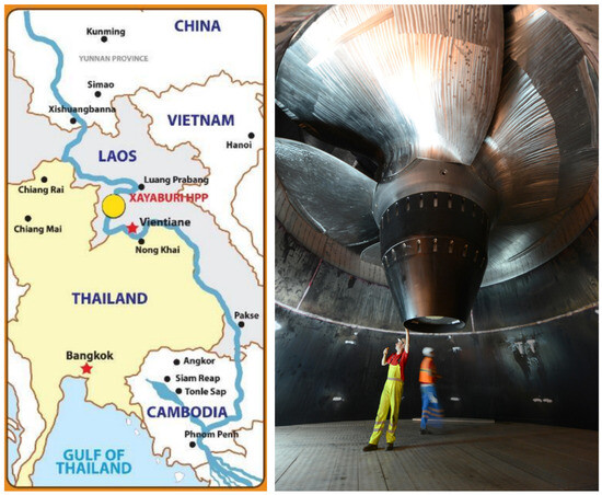
Figure 4.
Map showing location of the Xayaburi hydropower plant on the Mekong River in the Xayaburi Province of Lao PDR (left), as well as a perspective view of the tested Kaplan-type runner (not to scale) (right).
The power station consists of seven Kaplan-type turbines of 175 MW rated capacity, as well as one smaller Kaplan-type turbine of 60 MW, for a maximum capacity of 1284 MW and an estimated energy production of 7405 GWh. One of the 175 MW turbines was tested, which has a runner diameter (D) of 8.6 m, rotates at a constant rate of 83.33 revolutions per minute, and operates under a rated head (Hrated) of 28.5 m.
SF deployments were conducted onsite between 20–23 October 2022 at Unit 5. Two release elevations (labeled as top and bottom releases; see Table 1 and locations in Figure 3) were selected to test the influence of entrainment elevation on the passage conditions. The entrainment elevation is known to be of great significance for the biological effects of turbine flows on passing fish for two reasons. First, entrained fish are most likely adjusted to the water column depth they swim at before passage, and this parameter preconditions their sensitivity to the nadir pressure they encounter under the blades. Second, it is assumed that shallow (e.g., near-intake ceiling) releases likely encounter near-hub passages, whereas deeper releases (e.g., near-intake floor) pass near the shroud. Hydraulically, both radial regions are different, and local passage conditions may lead to different rates of bodily injury. For that reason, previous SF deployments [16,17] have selected release elevation as a treatment condition, and the present study conforms with this strategy as well.

Table 1.
Operational and release conditions during the SF deployments.
3.2. The Sensor Fish
The Sensor Fish (SF, shown in Figure 5) are deployed to serve as surrogates of fish passing through turbines. The SF measures hydraulic conditions during passage through flows influenced by turbines and other hydraulic infrastructure [14]. The SF is nearly cylindrical, has a diameter of 25 mm and a height of 90 mm, and weighs 42 g. The SF can record five minutes of the following physical quantities at a sampling rate of 2048 Hz:
- Linear acceleration (three components): analogue accelerometer with ±200 g range (g is earth’s gravity);
- Pressure: board-mounted unit, maximum value of 1.2 MPa;
- Rotational rate of change (three components): magnetometer (±2000° s−1 per axis).
The SF has a flash memory of 128 Mbit and a lithium battery of 110 mAh. The circuits operate within a range of 2.7 to 3.6 V. The SF has a recovery module that consists of two weights attached to each side of the SF with a fishing line that gets heated up when the SF enters the “retrieval” modus, which occurs after the recording phase has elapsed. The fishing line gets severed by the heating process, and weights are released, causing the SF to become positively buoyant and float to the water surface. Then, it emits its signal so that it can be radio-located by a crew in charge of retrieval. Particular to this deployment campaign, surrogate Sensor Fish were also constructed and field-tested as part of the preparation phase (Figure 5c).
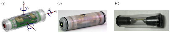
Figure 5.
(a) A CAD model of the Sensor Fish and (b) a photo of the Sensor Fish, taken from Deng et al. [14]. (c) A surrogate sensor fish was also fabricated and released during the preparation phase for deployments (see Section 3.3).
3.3. Deployments
Unit 5 of the Xayaburi HPP was selected for testing because trash racks of this unit are usually found very clean from debris during normal operations. SF units were brought into the turbine stream by means of a mechanism that was manufactured by the local HPP crew as part of the campaign preparations. The upstream portion of the release mechanism is shown in Figure 6. The release assembly consisted of a booster submersible pump that was connected to an HDPE pipe. This main pipe had an SF inserting slot that served to introduce the SF for each deployment event, after which the inserting slot valve was closed. Thereafter, the pump was switched on to produce the water jet that carried the SF down to the end of the ingress pipe. The terminus of the ingress pipe through which the SF was finally discharged into the intake stream was attached to the trash rack cleaning mechanism which, in regular operations, is displaced along the trash racks, thereby providing the advantage that the release elevation could be set with very high precision. This release strategy was selected over the alternative method of extending a long solid pipe into the intake because it minimized the possibility of potential turbine damage in the event of a breakup and detachment of pipe material.
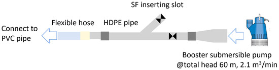
Figure 6.
Assembly of access point to bring sensors into the intake flow stream.
The procedure of an SF deployment is as follows. The deployment crew was split into two teams: upstream and downstream. The upstream team reported the SF ID and its frequency so that the downstream team could set up radio receivers. The upstream team prepared the SF for deployment in that they inserted a reacting chemical into the balloons, injected small amount of water, tied the balloons, and attached them to each end of the SF. Then, the SF was activated and brought into the inserting slot (Figure 6). The SF passed through the runner and turbine components and exited the draft tube at the moment at which the downstream team detected the exiting SF, either visually or with a radio receiver signal. The SF was retrieved, data were extracted, the memory card was cleaned, and SF programming settings were verified so that the SF unit was ready for another deployment. The recording time was set to 120 s.
During the preparation work, pre-deployments were also conducted with surrogate Sensor Fish—also known colloquially as dummy Sensor Fish, shown in Figure 5c—that were fabricated at the research laboratory of Charles Sturt University in Australia. Dummy Sensor Fish are of the same size (width and length) and buoyancy as the SF and allowed for the attachment of a balloon for retrieval. Dummy SF, however, do not contain electronics and, for that reason, lack the radio transmitter available in the standard SF. Another major difference between the models was the price per unit (an SF unit cost approximately USD 2500 in 2022, while the dummy Sensor Fish cost USD 20). The latter feature made dummy SF advantageous for testing the release and retrieval strategy without running the risk of losing commercial SF that are much more expensive.
3.4. SF Data Analysis
SF data were post-processed by using the Hydropower Biological Evaluation Toolset (HBET v2.0, Pacific Northwest National Laboratory, Richland, WA, USA) [38], which was developed to facilitate the handling of SF data, to analyze prescribed, fish-relevant hydraulic magnitudes, to elaborate reports in an automated manner, and to link key hydraulic outcomes to survival estimates via biological response models. One of the main features of HBET is the friendly user interface so that timing markers can be identified (see Section 5.2), which define the physical location where hydraulic stressors took place. The timing markers defined four spatial regions: (i) ingress (T0) to distributor entrance (T1), (ii) distributor entrance to runner entrance (T2), (iii) runner passage (T2 to T3), and (iv) draft tube entrance (T3) to draft tube exit (T4). SF do not record their location, and this must be inferred based on analyses of key features of the recordings. Timing markers were based on previous experience with SF post-processing as well as on the analysis of corresponding time series of pressure generated from passage simulations, from which physical location is always known. HBET outcomes relevant for the present study that were discussed in Section 2 are listed below:
- Pressure at ingress (T0);
- Pressure at distributor ingress (T1);
- Nadir pressure;
- Number of collision contacts detected at each transect within the turbine.
4. Flow and Passage Simulations
The magnitudes of nadir pressures and collision rates investigated in this study were also calculated via flow and passage simulations. Simulation-based assessments simultaneous with SF deployments are advantageous for at least three reasons. First, simulations provide a richer source of 3D flow information, which gave context to the measured hydraulic stressors. A validated simulation setup can assist in investigating remedies against flow conditions that negatively affect passage survivability. Second, simulations can assist in characterizing fish passage over a broader range of operational scenarios than the measured ones. This extrapolation can be done with a greater degree of certainty, provided that good agreement exists between SF- and simulation-based outcomes for those cases that did get measured. Lastly, simulation-based assessments are much more affordable and less logistically complex than field measurement campaigns.
The simulation-based assessment consists of modeling the geometric features of the turbine runner and components (Section 4.1), a selection of physics models that adequately represented actual physical phenomena (Section 4.2), the simulation of passage with streamlines, and the strategic post-processing of trajectory information (Section 4.3). It is important to emphasize that flow simulations conducted herein followed standard practices in the industry for designing turbine runners and components. This means that we did not optimize the simulation setup for conducting the current fish passage analysis but, instead, merely made use of a simulation setup defined during the turbine design phase.
4.1. Geometric Modeling
The 3D geometric model of the turbine was developed with NX 2306 (Siemens Digital Industries Software) to produce a water-tight domain that consisted of four regions (Figure 7): the intake, distributor, runner, and draft tube. All components were handled separately but were connected through interfaces to produce a continuous water passage. The intake is of semi-spiral type, and the inlet was set up further upstream to minimize the influence of the inflow on the flow calculations. The distributor contains 24 stay vanes and an equal number of guide vanes, which are tilted with respect to a vertical axis to further increase the efficiency of machine operations. The runner is five-bladed, and the elbow-type draft tube has two piers. The draft tube end was extended to minimize the influence of the outflow on the numerical flow calculations.
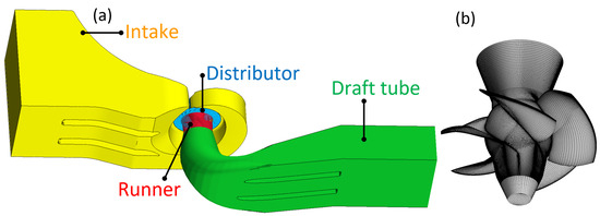
Figure 7.
(a) The 3D geometric model of the Xayaburi Kaplan turbine and (b) the mesh on the solid runner walls.
The computational domain was split into small volumes over which the numerical calculation is performed. Meshes consisted mostly of hexahedral cells and were generated with internal meshing tools specially tailored for the design of hydro turbine runners and components. The mesh sizes were 1.38 million, 14.16 million, 3.62 million, and 843.35 thousands for the intake, distributor, runner, and draft tube domains, respectively. The mesh sizes were selected based on a sensitivity test conducted during the design phase of the turbine. In addition, the turbine manufacturer has historically presented relevant work on the mesh sensitivity tests for hydraulic development of runners, draft tubes, and distributors for various projects [39,40,41]. From this experience, the mesh sizes to be implemented in flow simulations are an integral part of design protocols. Localized refinements on walls allowed for the implementation of a boundary layer treatment for flows near solid walls. Figure 7b shows the surface meshing on the runner blades and hub.
4.2. Flow Simulations
Simulations were conducted using CFX v2020 R2 (Ansys, Inc., Canonsburg, PA, USA), which allowed us to select the following physics models for flow analyses. A one-phase fluid medium in steady-state mode was assumed via the selection of the “Continuous Fluid” model for the material morphology. For modeling turbulent conditions, the - turbulence formulation as well as “first-order” numerics and a “high-resolution” advection scheme were selected. The “scalable” boundary layer model enabled the calculation of near-wall velocity conditions under the very variable cell resolutions that resulted from the mesh generation step. The turbine runner did not rotate during the flow simulation; instead, the runner motion was modeled by prescribing a localized reference frame with a rotational speed of 83.33 rpm. This local reference frame was applied to the volume and boundaries of the runner region, except for the shroud and the stationary part of the hub, where absolute velocity values were made equal to zero. Physical transitions between guide vane/runner and runner/draft tube resulted in a change of frame of reference, which was more accurately modeled by selecting the “stage (mixing-plane)” interface option, which averaged out the flow conditions circumferentially.
The solver implemented a “no-slip wall” boundary condition for all solid walls, with a “smooth wall” definition for wall roughness. The most upstream (intake inlet) boundary condition was governed by a fixed total pressure with flow direction normal to the boundary and a medium turbulence intensity of 5%. On the other hand, the most downstream boundary (outlet of the draft tube extension) was set up as an average static pressure that mimicked the actual hydrostatic pressure variation in the HPP. The pressure differential between the inlet and outlet boundaries reflected the net water head for each operating point. The net head is equal to in Table 1, minus the head losses at intake and tailrace, which were determined with an empirical relationship.
The numerical solution converged after 330 iterations using a “Physical Timescale” that followed a series of step functions internally developed for ensuring numerical stability in water turbine flow simulations. After convergence was reached, the solution stopped and produced three components of velocity, pressure, and two 3D fields describing the turbulent conditions, namely, the turbulent kinetic energy () and its rate of dissipation (). The simulations were run at physical model scale and, therefore, velocity and pressure at the prototype were estimated by following the principles of hydraulic similarity of discharge factor, speed factor, and cavitation number that are stipulated by the international standard IEC-60193 [42] for model acceptance tests.
4.3. Passage Simulations
After flows were calculated with CFD, streamlines were generated to represent Sensor Fish trajectories through the turbine flow. Streamlines consist of a set of points (XYZ coordinates) that are numerically calculated by following the instantaneous direction of fluid velocity at each point of the calculated 3D flow domain. Streamlines do not account for the surface and body forces that the surrounding fluid exerts on the SF unit; instead, they are invisible particles that are carried along with the fluid. The latter modeling simplification poses the question about whether streamlines suffice for accurately representing pathways through turbine flows. Alternatives have been proposed, for instance, by using Lagrangian particles or by representing fish as discrete elements with consideration of their body length and explicit wall contact modeling [29]. Nevertheless, the accuracy of all trajectory approximation methods (streamlines, Lagrangian particles, and discrete elements) has not been put to the test by directly comparing passage simulation outcomes with corresponding field data. Therefore, the present study serves as validation of the fish-related hydraulics generated via passage simulations with streamlines.
The starting point of streamlines (seeds) represents the point at which SF left the ingress pipe and entered the intake flow stream. Here, seeds were defined as a patch of points (XYZ coordinates) at the corresponding test elevation (top or bottom "target patch" as explained in Section 5.3). SF data provided an estimate of the start locations as explained in Section 5.3. Streamlines pass through all regions, but relevant information is collected from the passage transect through the runner.
For collision probability ( in Equation (2)), the three velocity components as well as coordinates were sampled at points where streamlines intersected a crossing plane defined over the leading edge of the blades (Group A in Figure 8, yellow cone). The thickness (T) was calculated based on a construction relationship that dictated the value of thickness as a function of radius (r). Since the r value at the moment of passage was calculated from the XYZ coordinates, the function could be applied. The SF length (L) was equal to 10 cm.
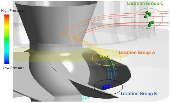
Figure 8.
Location of Group A shows the points at which streamlines pass a crossing plane; Group B shows the physical locations of nadir pressures; and Group C shows the pressure at the distributor entrance, with which the pressure drop () could be calculated.
For nadir pressures, we applied a minimum search function on the pressure time series of each streamline. This query for minimum pressure automatically yielded the physical location of nadir points as well, which is shown for some streamlines in the location of Group B in Figure 8. The lowest nadir pressures were mostly found on the suction side of the runner blade. Finally, the pressure value at the distributor entrance (location of Group C) was also sampled so that Equation (3) could be provided for each streamline.
5. Results
5.1. Data Collection
Table 2 summarizes the number of deployed sensors, lost units, damage sensors, and valid datasets that resulted from the deployment. Not every Sensor Fish that was deployed could be recovered, and very few of those that were recovered did not yield a valid dataset. Invalid datasets occurred for the following reasons; (a) some sensors recorded data over a period of time shorter than the stipulated 120 s, thereby yielding an incomplete dataset; (b) other sensors got stuck in the ingress pipe and came out of it in posterior rounds; (c) other sensors were recovered with an unexpected delay and showed signals that indicated that they got stuck in the distributor and came out minutes later with data collection for the intake only.
Table 2.
Equipment usage and collected sample.
For the purpose of comparing the statistical significance of the sample size, Table 3 shows the sample size per experimental treatment in Sensor Fish tests through large Kaplan-type turbines. Key characteristics of the turbines at each site are also given in the table. It is important that the number of valid datasets collected at the Xayaburi HPP for the present study corresponded to a minimum sample size requirement according to guidelines from previous measurement campaigns with SF.
Table 3.
Sample size per treatment and characteristics of the turbine runner for large hydro Kaplan projects where SF have been previously deployed and reported.
5.2. Example of a Passage
A successfully collected dataset consisted of time series of absolute pressure (shown in green in both plots of Figure 9), magnitude of linear acceleration (blue series in top plot), and of angular rotation (red series in bottom plot). We describe herein patterns that were consistently observed through most datasets. SF units do not record the location, and the patterns from SF measurements and CFD-based time series discussed in this section assisted us in identifying passage transects (intake, guide vane, runner, and draft tube). The start and end of passage through each component are referred to as “timing markers” and were defined as follows.
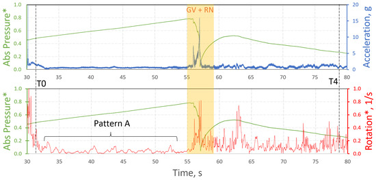
Figure 9.
Example of a Sensor Fish passage. The upper plot shows time series of absolute pressure ( in Equation (4)) and acceleration, whereas the bottom plot shows time series of absolute pressure and rotations. A close-up of the pressure time series during distributor and runner passage is shown in Figure 10.
When SF were moving down the ingress pipe, continuous contacts with the pipe walls generated spikes until the SF reached the terminus of the pipe. This instant was set as the beginning of passage (or T0) and was consistent with the start of a free SF motion through the intake without exhibiting any major acceleration spike. During the transect at the intake, the rotational speed exhibited a very regular oscillation (see Pattern A in Figure 9), which subsided as the SF approached the entrance of the distributor. Passage through the distributor and runner was characterized by very rapid and large pressure changes, which are depicted with more detail in the Figure 10. To identify the instant of transitions for intake/distributor (T1), distributor/runner (T2), and runner/draft tube (T3), we resorted to corresponding time series of absolute pressure calculated from CFD and passage simulations (inset in Figure 10), which offered the advantage that the position was known at all times. This latter feature facilitated the definition of transition points (squared markers) on the CFD-simulated pressure history of the inset of Figure 10. Patterns were in this way visible in both time series. The entrance to the distributor (Pattern B) was accompanied by a very mild drop in pressure with a nearly immediate recovery. This pattern defined timing marker T1. Thereafter, absolute pressure decreased very rapidly until a minimum pressure value was reached (nadir pressure, Pattern C). Simulation-based visualizations have shown that nadir points always occurred under the suction side of the runner blades [24]. Therefore, we could estimate through simulations the averaged time () elapsed between the entrance to the runner (T2) and the occurrence of nadir pressure. The average from all simulated streamlines was subtracted from the nadir pressure occurrence time for each SF dataset to determine the timing marker T2. A similar strategy was implemented to estimate the time elapsed between nadir and entrance to draft tube () from simulations. In this case, was added to the nadir pressure occurrence time from SF data to determine the timing marker T3 for each dataset. The CFD-estimated time necessary for draft tube passage was added to T3 for marking the end of passage (T4).
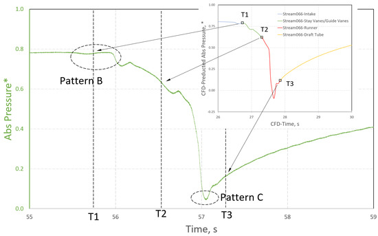
Figure 10.
Close-up of the pressure time series with a focus on distributor and runner passage. The inset shows corresponding computer-generated time series of pressure ( in Equation (4)) with CFD and streamlines, which assist in marking the instants where SF entered the distributor (T1), the runner (T2), and the draft tube (T3).
Most sensors yielded time series that showed the above-mentioned features, with only a few exhibiting minor deviations. For instance, some SF did not record a very strong, regular, fluctuating angular velocity at the instant of ingress (Pattern A in Figure 9 was missing). Nevertheless, T0 was estimated as the instant when acceleration spikes caused by collisions inside the ingress pipe disappeared. Other recordings exhibited a relatively flat time series of absolute pressure from ingress to the distributor. This, however, did not preclude the selection of the timing markers that were necessary for data analyses.
5.3. Pressure Analysis
Because the start location of streamlines influenced simulation-based outcomes considerably, the timing markers T0 from SF data were used to estimate the streamline seed locations. To account for the random influence of turbulence on SF pathways, seeds were defined as a “patch” of points. An alternative to the “patch” would be a single point that would result in a single streamline, which would preclude the variability observed from SF measurements. Theoretically, the patch should be centered at the middle of the center bay and at the intended elevation (labeled as “target patch” in Figure 11). A “target patch” did not, however, materialize in the field because SF were actually discharged into the intake flows with a downwards movement. Therefore, the actual seed locations must be estimated based on the ingress elevations of SF. Flow simulations showed that pressures at ingress (T0) behaved hydrostatically, which in turn meant that the ingress depth could be estimated. The SF data post-processing then yielded a sample of ingress elevations for each release condition. With this sample, a vertical distribution of seeds was generated to define the “actual patch” of seeds, as shown in Figure 11. Notice that the deviation between target and actual elevations was greater for the top than for the bottom releases. The water jet had to overcome a smaller water column for top releases than for the bottom ones. This resulted in discharges into the intake stream with a greater velocity at the top than at the bottom releases. Ultimately, the “actual patch” was used as streamline seeds.
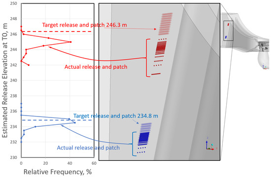
Figure 11.
Distributions of estimated release elevations based on pressure measurement at T0 for all releases.
Nadir pressures (shown in Pattern C of Figure 10) for all passage events, for both release locations, and for both evaluation methods are shown in Figure 12 as cumulative proportions. Results are presented in a normalized form, but no sub-atmospheric pressures were recorded. The chart also shows that the largest nadir values were approximately and for the bottom and top releases, respectively. The nadir pressure environment was clearly distinct as a function of release location. The bottom releases yielded lower nadir pressures than the top releases; median values between the two distributions differed by approximately .
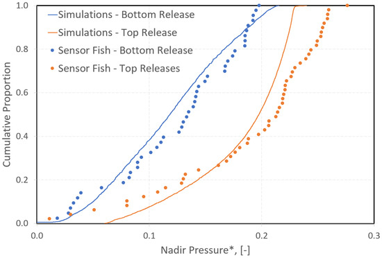
Figure 12.
Cumulative distributions of both simulated (with CFD) and measured (with SF) nadir pressures are shown for both release elevations. Pressures were normalized according to Equation (4).
The corresponding simulation-based distributions exhibited a very satisfactory agreement with field measurements with SF. Such agreement was stronger between distributions from the bottom releases than from the top releases. The largest deviations between SF and simulation-based outcomes were found at the end of both distribution (near-cumulative proportion equal to 1.0). Regarding the nadir pressure variability, the simulation-based method produced less variability than the SF measurements for the top releases, but both methods yielded nearly the same variability for the bottom release treatment.
Simulations allowed us to identify physical locations of nadir pressures (Figure 13). Nadir pressures were found mostly under the runner, before the transition to the draft tube took place. The closer the streamlines came to the blade surface, the lower the nadir pressure value was. Regarding the radial location of nadir points, top releases tended to yield nadir points closer to the hub than bottom releases did. The very few nadir pressures that were extremely low according to simulation predictions were associated with streamline passage though gaps, where the most extreme pressure changes were found. None of the SF recordings registered such low pressure values, which was an indication that the selected release locations did not yield any passage near gaps.
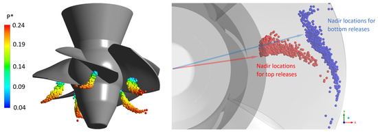
Figure 13.
Nadir pressure points from top releases are shown on the left colored by pressure value (dimensionless), whereas the radial locations of nadir points from both releases are on the right.
Pressure drops between the entrance to the distributor and nadir points are shown in Figure 14 from both SF measurements and simulation estimates. Both methods showed a tendency for bottom releases to yield greater pressure drops than top releases did. The difference in median values for both treatments was approximately 0.08. The prediction power for reproducing varies considerably. Accuracy of prediction from top releases was poorer than from bottom releases. The largest deviations between CFD estimates and SF measurements were observed for the lowest values (near-cumulative proportion equal to 0.0) arising from top releases, with the largest deviation being equal to 0.04 kPa.
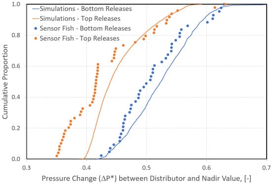
Figure 14.
Cumulative distributions of both simulated (with CFD) and measured (with SF) (*, dimensionless form) are shown for both release elevations.
5.4. Collision Analysis
The post-processing software for SF data analysis (HBET v2.0) attributed the occurrence of acceleration spikes to either (i) shear or (ii) strike events. The categorization was done automatically by HBET and was based on the intensity and timing of the time series of acceleration magnitude [38]. The absolute number of both types of events as well as the percentile (relative to the number of valid datasets) are summarized in Table 4 and Table 5 for the top and bottom releases, respectively. The outcomes from the two treatments have in common that neither shear nor strike events were recorded during intake passage. Shear events were also not frequent and were only present in the runner region. On the other hand, strike events were detected in the distributor, runner, and draft tube. The runner was the region where both types of contact events occurred with the greatest frequency. We reported not only the number of strike events but also the count of colliding SF, a differentiation that was important for comparing measurements and simulation outcomes. Therefore, it is necessary to clarify each reported quantity in Table 4 and Table 5. A single SF passage could yield various strike events during runner passage. All such events were summed up and reported under “strike events”, but the SF itself counted as a single “colliding SF” in Table 4 and Table 5. The count of colliding sensors was needed because the probabilistic model upon which simulation-based estimates were based, Equation (2), ignores the occurrence of multiple collision events during the same passage. In addition, collision probability in Equation (2) considers only collisions on the runner, and this is why the number of colliding sensors was only reported for the runner (). Most studies consider collisions on runners to be the most critical during turbine passage, while collisions on the distributor and draft tube attract less attention. Runner collision rates were 8.2–9.3%.
Table 4.
Summary of occurrence and intensity of contact events from all SF from top releases.
Table 5.
Summary of occurrence and intensity of contact events from all SF from bottom releases.
Simulation-based estimates consisted of a sample of collision probabilities calculated with Equation (2). This numerical sample size was as large as the number of streamlines and totaled approximately 3600 probability values for each release elevation. This allowed us to plot cumulative proportion distributions (Figure 15, left) that show features of both central tendency and dispersion for the collision probability. According to the model outcomes, top releases yielded lower collision probabilities than bottom releases did, as well as a greater variability in collision probabilities. The difference in median values between both distributions was equal to 3.7%. SF data yielded only two values of collision frequency, and these are plotted in Figure 15 as vertical dashed lines. It should be noted that the current status of the SF technology does not allow for a clear differentiation between contacts on the leading edge of the blade and contacts elsewhere on the blade surface. In addition, the sample sizes of SF data do not allow for a conclusive argument that the relatively small difference between SF-recorded collision frequencies was the result of the experimental treatment, i.e., that the release location influences collision frequency. On the other hand, we can definitively infer that the probabilistic model, in combination with the sampling strategy for passage conditions based on simulations, yields values of collision rate that satisfactorily approximate the magnitude of collision frequency measured with SF. The latter argument increased our level of confidence in the probabilistic model of Equation (2) and indicates that a simplified geometric representation of passage is an adequate first approximation of the the complex body–fluid interactions that occur as Sensor Fish pass rotating runners.
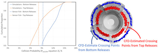
Figure 15.
On the left, outcomes of collision frequency from Sensor Fish (vertical dashed lines) and collision probability (distributions) from simulation-based estimates for both release elevations. On the right, all crossing points above the runner were estimated via simulations for both release elevations.
Simulated crossing points were collected from streamlines as they approached the leading edge of the blade and are shown on the right side of Figure 15. Top releases yielded crossing points near the hub, while bottom releases produced passages near the discharge ring. This difference in radial location influenced , mainly because and V were 10–15% lower at near-discharge locations than at near-hub passages. These lower near-discharge velocities increased the time that an SF would take to pass through the crossing plane, thereby increasing the probability that SF would collide on the blades.
6. Discussion
Overall, SF measurements provided an unambiguous characterization of both the nadir pressure and collision environments to which fish could potentially be exposed during passage at the Xayaburi HPP. Based on the fact that simulation-based outcomes provided a satisfactory agreement with measurements for pressure and collision stressors, our engineering judgment suggests that the sample size collected in the field campaign was sufficient for an adequate characterization of passage conditions. This is reinforced by the fact that the sample sizes in the present study are similar to those collected in previous measurement campaigns in large Kaplan runners. Advantageous in the present assessment is that the simulation method provided physical context with which SF data could be interpreted with greater certainty.
Time series of pressure can be explained in the context of flow phenomena that are known by hydraulic developers of runners and turbine components. For instance, pressures at the instant of ingress are strongly linked to the hydrostatic pressure conditions prevailing at the intake. Nadir pressures, on the other hand, always occur below the suction side of the runner blades, a surface that is carefully designed to avoid the appearance of cavitation during normal operations. The SF outcomes for pressure were satisfactorily reproduced by simulation results and, therefore, provided a solid reference that can be used to propose pressure time series for laboratory experimentation of the sensitivity of local fish of the Mekong River to barotrauma. Such experiments have already been conducted for fish species in regions with temperate climate [9,43] but equivalent biological data are necessary for fish species of the Mekong River as well as for those species in regions of the world where hydropower developments are taking place. Dose–response biological relationships will further strengthen the value of fish-relevant hydraulic information collected with SF, since linking pressure conditions to likelihood of survival would allow researchers to conduct full biological assessments either for the entire operating range of a constructed turbine or for proposed designs in future hydropower sites.
Collisions did not depend on release elevation, and this was consistent with modeling estimates and SF-based outcomes. One improvement in the collision assessment consists of investigating collision intensity that could be achieved via impact velocity calculations based on simulations or via novel post-processing algorithms that account for all time series collected by SF. Collision intensity, characterized by impact velocity in all biological models of Pflugrath et al. [44], is a driving factor for estimating the likelihood of mortal injury of fish due to mechanical contact with the runner blades. Another relevant outcome from this study is that SF data post-processing showed collisions on stationary components, namely the distributor and draft tube. This evidence calls for laboratory experimentation to test the hypothesis that collisions on stationary walls are of no biological consequence.
Top releases yielded greater dispersion of nadir pressures and collision probabilities than bottom releases did, which is an indication that top releases were subject to a greater variety of flow conditions. In addition, top releases produced near-hub runner passages that exhibited greater nadir pressures, lower pressure drops, and slightly lower collision probabilities. All these trends are desirable features for fish passage, which means that, qualitatively, top releases will give rise to safer passage through the runner. However, a quantitative statement can only be formulated by resolving the connection between hydraulic stressors and consequential biological effects for local species via laboratory experimentation. Magnitudes reported in this study can be used for the experimental design of the biological tests.
The SF records three components of the rotational velocity, which were analyzed but not included in the present work because the simulation-based counterpart was not carried out. Streamlines used to approximate the SF pathways do not rotate and, therefore, cannot yield rotational velocities that could be compared with SF measurements. Rotations of the sensor, or of any object moving through a fluid flow, are the result of surface and body forces acting on the sensor, as well as of its inertial properties. Furthermore, rotations themselves have an influence on the surrounding fluid motion, thereby requiring a coupled formulation for flow simulations. Direct simulations of rotating motion for inertial cylinders that are the size of the SF are computationally expensive and are still not feasible for examining passage of SF through a turbine. Even if we were able to predict rotations via simulation techniques, their biological consequence remains largely unexplored, since the mortality associated with rotations cannot be assessed with the degree of certainty to which the effects of pressure and collisions can be evaluated. Therefore, rotation measurements and corresponding simulations deserve a full study with at least two major steps. A first step would be to characterize the magnitudes of rotational speed at various operating conditions and for various designs, and a second step would consist of linking such magnitudes to the biological response.
Lastly, this study carried out flow and passage simulations by following standard practices in the industry for designing turbines, even though it is known that various advanced computational techniques have increased the prediction accuracy of flow phenomena in turbine flows, namely eddy-resolving methods, dynamic runner simulations, Lagrangian particle tracking, and particle contact modeling, to name a few. While these simulation techniques have been offered as an advancement for flow simulations in practical industrial processes [45], hydraulic turbine development in industrial settings primarily relies on the strategies presented in Section 4 due to the considerable savings in computational expense that they bring about. The present study increased the certainty of the use of standard simulation protocols to achieve an adequate characterization of pressure and collision environments that fish may experience during turbine passage. This greater certainty in prediction power, in turn, considerably increases the confidence of turbine engineers to develop new technology based on safer fish passage conditions.
The present work was the first step for planning and executing laboratory experiments through which the biological response of local fish to the measured hydraulic stressors can be determined via dose–response experiments [9,43,44]. The Mekong River is extremely biodiverse and, as of today, little information is know about the effects that turbine passage could have on the likelihood of survival (an example can be found in the work of Colotelo et al. [12]). The first step to investigate such effects consists of knowing what hydraulic stressor magnitudes fish experience during passage. With the present work, the fish-relevant hydraulic magnitudes were measured and simulated at the Xayaburi HPP.
7. Conclusions
The Mekong River is an active region for developing hydropower production in the upcoming decades. Fish protection has taken central stage, and fish biologists and environmental scientists have pointed out that a hydraulic characterization of fish passage conditions (e.g., with sensors) through operating turbines should ideally precede direct fish survival assessments (e.g., with live fish samples passed through turbines). The present study conducted the characterization of fish-relevant hydraulics through the large Kaplan turbine of the Xayaburi HPP by means of two methods: the deployment of SF in the field and simulations of flow conditions and passage events. This hydraulic characterization is an essential intermediate step to ultimately link turbine operations and their consequential effects on survivability, which can assist in making well-informed operational decisions at the HPP.
The experimental protocol conformed with the general guidelines from previous studies and provided evidence that the SF release elevation—a surrogate of fish entrainment location into the turbine flows—influences the pressure conditions fish are exposed to during passage. Whether or not these recorded onsite pressure conditions and their variability are relevant for the survivability of local fish of the Mekong River can only be known via subsequent biological sensitivity tests in laboratory experiments. The present work collected sufficient data to inform the experimental design of such tests. The sensitivity of the frequency of collisions on the runner to the release elevation was relatively small since both treatments yielded low collision rates.
The second method implemented herein, flow and passage simulations, is gaining acceptance by environmental authorities and scientists, which makes it essential to provide evidence about their accuracy. Validations of simulated outcomes can only be achieved by conducting both SF measurements and corresponding simulations on the same study case. The present work demonstrated that flow and passage simulations can satisfactorily reproduce nadir pressures, pressure drops, and collision rates through the Kaplan turbine of Xayaburi HPP. More important, simulation strategies were based on industry practices, which have been optimized over the years to reduce computational expense while maintaining an acceptable prediction power of flow phenomena. The agreement between measurements and simulations contributed to a gain in confidence for using the simulation setup for addressing associated questions of environmental relevance. For instance, onsite partners were already informed about equivalent fish-relevant hydraulics through the Kaplan turbines to be installed in another hydropower station currently under construction.
First-hand data collection with sensors allows turbine engineers to field-test their design assumptions related to safe turbine passage. The more understanding industry has about the relationships between the design and operation of a turbine and its biological effect in the field, the more likely it will be that the industry can unfold the potential and accelerate the development of environmentally enhanced turbine technology with minimum impact on natural resources.
Author Contributions
P.R.-G. contributed to this article with formal analysis, investigation, validation, visualization, writing—original draft, writing review and editing. T.P. contributed with conceptualization, methodology, investigation and supervision. R.R. contributed with conceptualization and methodology. W.R. contributed with conceptualization, methodology, investigation, supervision, writing—review and editing. R.P. contributed with supervision, project administration and funding acquisition. M.R. contributed with conceptualization, methodology, supervision, project administration and funding acquisition. L.J.B. contributed with conceptualization, methodology, supervision, project administration, funding acquisition and writing—review and editing. All authors have read and agreed to the published version of the manuscript.
Funding
This research is part of the project “Assessing fisheries mitigation measures at Xayaburi Dam in Lao PDR” sponsored by the Australian Centre for International Agricultural Research (FIS/2017/017).
Data Availability Statement
The data presented in this study are available on request from the corresponding author. The data are not publicly available due to ownership rights.
Conflicts of Interest
Co-authors Pedro Romero-Gomez and Rudolf Peyreder are employees of the company Andritz Hydro GmbH; co-authors Thanasak Poomchaivej, Rajesh Razdanand Michael Raeder are employees of the company CKPower Public Company Limited. The remaining authors declare that the research was conducted in the absence of any commercial or financial relationships that could be construed as a potential conflict of interest.
References
- IRENA. Renewable Energy Statistics 2021; Technical report; International Renewable Energy Agency: Masdar City, United Arab Emirates, 2021. [Google Scholar]
- Zarfl, C.; Lumsdon, A.E.; Berlekamp, J.; Tydecks, L.; Tockner, K. A global boom in hydropower dam construction. Aquat. Sci. 2015, 77, 161–170. [Google Scholar] [CrossRef]
- Baumgartner, L.J.; Daniel Deng, Z.; Thorncraft, G.; Boys, C.A.; Brown, R.S.; Singhanouvong, D.; Phonekhampeng, O. Perspective: Towards environmentally acceptable criteria for downstream fish passage through mini hydro and irrigation infrastructure in the Lower Mekong River Basin. J. Renew. Sustain. Energy 2014, 6, 012301. [Google Scholar] [CrossRef]
- Geist, J. Green or red: Challenges for fish and freshwater biodiversity conservation related to hydropower. Aquat. Conserv. Mar. Freshw. Ecosyst. 2021, 31, 1551–1558. [Google Scholar] [CrossRef]
- Twardek, W.M.; Cowx, I.G.; Lapointe, N.W.; Paukert, C.; Beard, T.D.; Bennett, E.M.; Browne, D.; Carlson, A.K.; Clarke, K.D.; Hogan, Z.; et al. Bright spots for inland fish and fisheries to guide future hydropower development. Water Biol. Secur. 2022, 1, 100009. [Google Scholar] [CrossRef]
- Larinier, M.; Dartiguelongue, J. La circulation des poissons migrateurs: Le transit à travers les turbines des installations hydroélectriques. Bulletin Français Pêche Pisciculture 1989, 312, 312–313. [Google Scholar] [CrossRef]
- Pracheil, B.M.; DeRolph, C.R.; Schramm, M.P.; Bevelhimer, M.S. A fish-eye view of riverine hydropower systems: The current understanding of the biological response to turbine passage. Rev. Fish Biol. Fish. 2016, 26, 153–167. [Google Scholar] [CrossRef]
- Ferguson, J.W.; Absolon, R.F.; Carlson, T.J.; Sandford, B.P. Evidence of delayed mortality on juvenile Pacific salmon passing through turbines at Columbia River dams. Trans. Am. Fish. Soc. 2006, 135, 139–150. [Google Scholar] [CrossRef]
- Brown, R.S.; Carlson, T.J.; Gingerich, A.J.; Stephenson, J.R.; Pflugrath, B.D.; Welch, A.E.; Langeslay, M.J.; Ahmann, M.L.; Johnson, R.L.; Skalski, J.R.; et al. Quantifying Mortal Injury of Juvenile Chinook Salmon Exposed to Simulated Hydro-Turbine Passage. Trans. Am. Fish. Soc. 2012, 141, 147–157. [Google Scholar] [CrossRef]
- Bevelhimer, M.S.; Pracheil, B.M.; Fortner, A.M.; Saylor, R.; Deck, K.L. Mortality and injury assessment for three species of fish exposed to simulated turbine blade strike. Can. J. Fish. Aquat. Sci. 2019, 76, 2350–2363. [Google Scholar] [CrossRef]
- Baumgartner, L.J.; Thorncraft, G.; Phonekhampheng, O.; Boys, C.; Navarro, A.; Robinson, W.; Brown, R.; Deng, Z. High fluid shear strain causes injury in silver shark: Preliminary implications for Mekong hydropower turbine design. Fish. Manag. Ecol. 2017, 24, 193–198. [Google Scholar] [CrossRef]
- Colotelo, A.H.; Mueller, R.; Harnish, R.; Martinez, J.J.; Phommavong, T.; Phommachanh, K.; Thorncraft, G.; Baumgartner, L.; Hubbard, J.; Rhode, B.; et al. Injury and mortality of two Mekong River species exposed to turbulent shear forces. Mar. Freshw. Res. 2018, 69, 1945–1953. [Google Scholar] [CrossRef]
- Deng, Z.; Carlson, T.J.; Duncan, J.P.; Richmond, M.C. Six-degree-of-freedom sensor fish design and instrumentation. Sensors 2007, 7, 3399–3415. [Google Scholar] [CrossRef]
- Deng, Z.; Lu, J.; Myjak, M.; Martinez, J.J.; Tian, C.; Morris, S.; Carlson, T.; Zhou, D.; Hou, H. Design and implementation of a new autonomous sensor fish to support advanced hydropower development. Rev. Sci. Instruments 2014, 85, 115001. [Google Scholar] [CrossRef]
- Deng, Z.; Carlson, T.J.; Duncan, J.P.; Richmond, M.C.; Dauble, D.D. Use of an autonomous sensor to evaluate the biological performance of the advanced turbine at Wanapum Dam. J. Renew. Sustain. Energy 2010, 2, 053104. [Google Scholar] [CrossRef]
- Dauble, D.D.; Deng, Z.; Richmond, M.C.; Moursund, R.A.; Carlson, T.J.; Rakowski, C.L.; Duncan, J.P. Biological Assessment of the Advanced Turbine Design at Wanapum Dam, 2005; Technical report; Pacific Northwest National Lab. (PNNL): Richland, WA, USA, 2007. [Google Scholar]
- Martinez, J.; Deng, Z.; Titzler, P.; Duncan, J.; Lu, J.; Mueller, R.; Tian, C.; Trumbo, B.; Ahmann, M.; Renholds, J. Hydraulic and biological characterization of a large Kaplan turbine. Renew. Energy 2019, 131, 240–249. [Google Scholar] [CrossRef]
- Fu, T.; Deng, Z.D.; Duncan, J.P.; Zhou, D.; Carlson, T.J.; Johnson, G.E.; Hou, H. Assessing hydraulic conditions through Francis turbines using an autonomous sensor device. Renew. Energy 2016, 99, 1244–1252. [Google Scholar] [CrossRef]
- Martinez, J.J.; Deng, Z.D.; Klopries, E.M.; Mueller, R.P.; Titzler, P.S.; Zhou, D.; Beirao, B.; Hansten, A.W. Characterization of a siphon turbine to accelerate low-head hydropower deployment. J. Clean. Prod. 2019, 210, 35–42. [Google Scholar] [CrossRef]
- Boys, C.A.; Pflugrath, B.D.; Mueller, M.; Pander, J.; Deng, Z.D.; Geist, J. Physical and hydraulic forces experienced by fish passing through three different low-head hydropower turbines. Mar. Freshw. Res. 2018, 69, 1934–1944. [Google Scholar] [CrossRef]
- Abeykoon, C. Modelling and optimisation of a Kaplan turbine—A comprehensive theoretical and CFD study. Clean. Energy Syst. 2022, 3, 100017. [Google Scholar] [CrossRef]
- Khare, R.; Prasad, V.; Kumar, S. CFD approach for flow characteristics of hydraulic francis turbine. Int. J. Eng. Sci. Technol. 2010, 2, 3824–3831. [Google Scholar]
- Ventikos, Y.; Sotiropoulos, F.; Fisher, R., Jr.; March, P.; Hopping, P. A CFD framework for environmentally-friendly hydroturbines. In Waterpower’99: Hydro’s Future: Technology, Markets, and Policy; American Society of Civil Engineers: Las Vegas, NV, USA, 1999. [Google Scholar]
- Richmond, M.C.; Serkowski, J.A.; Rakowski, C.; Strickler, B.; Weisbeck, M.; Dotson, C. Computational tools to assess turbine biological performance. Hydro Rev. 2014, 33, 88–97. [Google Scholar]
- Richmond, M.C.; Serkowski, J.A.; Ebner, L.L.; Sick, M.; Brown, R.S.; Carlson, T.J. Quantifying barotrauma risk to juvenile fish during hydro-turbine passage. Fish. Res. 2014, 154, 152–164. [Google Scholar] [CrossRef]
- Müller, S.; Cleynen, O.; Hoerner, S.; Lichtenberg, N.; Thévenin, D. Numerical analysis of the compromise between power output and fish-friendliness in a vortex power plant. J. Ecohydraulics 2018, 3, 86–98. [Google Scholar] [CrossRef]
- Zhu, G.; Guo, Y.; Feng, J.; Gao, L.; Wu, G.; Luo, X. Analysis and reduction of the pressure and shear damage probability of fish in a Francis turbine. Renew. Energy 2022, 199, 462–473. [Google Scholar] [CrossRef]
- Klopries, E.M.; Schüttrumpf, H. Mortality assessment for adult European eels (Anguilla Anguilla) during turbine passage using CFD modelling. Renew. Energy 2020, 147, 1481–1490. [Google Scholar] [CrossRef]
- Singh, R.K.; Romero-Gomez, P.; Colotelo, A.H.; Perkins, W.A.; Richmond, M.C. Computational studies of hydraulic stressors for biological performance assessment in a hydropower plant with Kaplan turbine. Renew. Energy 2022, 199, 768–781. [Google Scholar] [CrossRef]
- Coutant, C.C.; Whitney, R.R. Fish behavior in relation to passage through hydropower turbines: A review. Trans. Am. Fish. Soc. 2000, 129, 351–380. [Google Scholar] [CrossRef]
- Čada, G.F. The development of advanced hydroelectric turbines to improve fish passage survival. Fisheries 2001, 26, 14–23. [Google Scholar] [CrossRef]
- Hogan, T.W.; Cada, G.F.; Amaral, S.V. The status of environmentally enhanced hydropower turbines. Fisheries 2014, 39, 164–172. [Google Scholar] [CrossRef]
- Mueller, M.; Pander, J.; Geist, J. Evaluation of external fish injury caused by hydropower plants based on a novel field-based protocol. Fish. Manag. Ecol. 2017, 24, 240–255. [Google Scholar] [CrossRef]
- Mueller, M.; Sternecker, K.; Milz, S.; Geist, J. Assessing turbine passage effects on internal fish injury and delayed mortality using X-ray imaging. PeerJ 2020, 8, e9977. [Google Scholar] [CrossRef] [PubMed]
- Doyle, K.E.; Ning, N.; Silva, L.G.; Brambilla, E.M.; Deng, Z.D.; Fu, T.; Boys, C.; Robinson, W.; Du Preez, J.A.; Baumgartner, L.J. Survival estimates across five life stages of redfin (Perca fluviatilis) exposed to simulated pumped-storage hydropower stressors. Conserv. Physiol. 2022, 10, coac017. [Google Scholar] [CrossRef] [PubMed]
- Brown, R.S.; Colotelo, A.H.; Pflugrath, B.D.; Boys, C.A.; Baumgartner, L.J.; Deng, Z.D.; Silva, L.G.; Brauner, C.J.; Mallen-Cooper, M.; Phonekhampeng, O.; et al. Understanding barotrauma in fish passing hydro structures: A global strategy for sustainable development of water resources. Fisheries 2014, 39, 108–122. [Google Scholar] [CrossRef]
- Martinez, J.; Deng, Z.D.; Tian, C.; Mueller, R.; Phonekhampheng, O.; Singhanouvong, D.; Thorncraft, G.; Phommavong, T.; Phommachan, K. In situ characterization of turbine hydraulic environment to support development of fish-friendly hydropower guidelines in the lower Mekong River region. Ecol. Eng. 2019, 133, 88–97. [Google Scholar] [CrossRef]
- Hou, H.; Deng, Z.D.; Martinez, J.J.; Fu, T.; Duncan, J.P.; Johnson, G.E.; Lu, J.; Skalski, J.R.; Townsend, R.L.; Tan, L. A hydropower biological evaluation toolset (HBET) for characterizing hydraulic conditions and impacts of hydro-structures on fish. Energies 2018, 11, 990. [Google Scholar] [CrossRef]
- Vu, T.; Gauthier, M.; Nennemann, B.; Wallimann, H.; Deschênes, C. CFD analysis of a bulb turbine and validation with measurements from the BulbT project. IOP Conf. Ser. Earth Environ. Sci. 2014, 22, 022008. [Google Scholar] [CrossRef]
- Devals, C.; Vu, T.; Zhang, Y.; Dompierre, J.; Guibault, F. Mesh convergence study for hydraulic turbine draft-tube. IOP Conf. Ser. Earth Environ. Sci. 2016, 49, 082021. [Google Scholar] [CrossRef]
- Braun, O.; Horisberger, B.; Ruchonnet, N.; Taruffi, A.; Gehrer, A. Validation of CFD analysis of acoustic effects in pump-turbine runners. IOP Conf. Ser. Earth Environ. Sci. 2019, 240, 062011. [Google Scholar] [CrossRef]
- IEC 60193:2019; Hydraulic Turbines, Storage Pumps, and Pump-Turbines. Model Acceptance Tests. International Electrotechnical Commission: Geneva, Switzerland, 1999.
- Pflugrath, B.D.; Boys, C.A.; Cathers, B. Predicting hydraulic structure-induced barotrauma in Australian fish species. Mar. Freshw. Res. 2018, 69, 1954–1961. [Google Scholar] [CrossRef]
- Pflugrath, B.D.; Saylor, R.; Engbrecht, K.M.; Mueller, R.P.; Stephenson, J.R.; Bevelhimer, M.; Pracheil, B.M.; Colotelo, A.H. Biological Response Models: Predicting Injury and Mortality of Fish during Downstream Passage through Hydropower Facilities; Technical report; Pacific Northwest National Lab. (PNNL): Richland, WA, USA, 2021. [Google Scholar]
- Li, L.; Xu, W.; Tan, Y.; Yang, Y.; Yang, J.; Tan, D. Fluid-induced vibration evolution mechanism of multiphase free sink vortex and the multi-source vibration sensing method. Mech. Syst. Signal Process. 2023, 189, 110058. [Google Scholar] [CrossRef]
Disclaimer/Publisher’s Note: The statements, opinions and data contained in all publications are solely those of the individual author(s) and contributor(s) and not of MDPI and/or the editor(s). MDPI and/or the editor(s) disclaim responsibility for any injury to people or property resulting from any ideas, methods, instructions or products referred to in the content. |
© 2024 by the authors. Licensee MDPI, Basel, Switzerland. This article is an open access article distributed under the terms and conditions of the Creative Commons Attribution (CC BY) license (https://creativecommons.org/licenses/by/4.0/).