Abstract
This study focuses on optimizing precipitation forecast induced by tropical cyclones (TCs) in the Northwest Pacific region, with lead times ranging from 6 to 72 h. The research employs deep learning models, such as U-Net, UNet3+, SE-Net, and SE-UNet3+, which utilize precipitation forecast data from the Global Forecast System (GFS) and real-time GFS environmental background data using a U-Net structure. To comprehensively make use of the precipitation forecasts from these models, we additionally use probabilistic matching (PM) and simple averaging (AVR) in rainfall prediction. The precipitation data from the Global Precipitation Measurement (GPM) Mission serves as the rainfall observation. The results demonstrate that the root mean squared errors (RMSEs) of U-Net, UNet3+, SE-UNet, SE-UNet3+, AVR, and PM are lowered by 8.7%, 10.1%, 9.7%, 10.0%, 11.4%, and 11.5%, respectively, when compared with the RMSE of the GFS TC precipitation forecasts, while the mean absolute errors are reduced by 9.6%, 11.3%, 9.0%, 12.0%, 12.8%, and 13.0%, respectively. Furthermore, the neural network model improves the precipitation threat scores (TSs). On average, the TSs of U-Net, UNet3+, SE-UNet, SE-UNet3+, AVR, and PM are raised by 12.8%, 21.3%, 19.3%, 20.7%, 22.5%, and 22.9%, respectively, compared with the GFS model. Notably, AVR and PM outperform all other individual models, with PM’s performance slightly better than AVR’s. The most important feature variables in optimizing TC precipitation forecast in the Northwest Pacific region based on the UNet-based neural network include GFS precipitation forecast data, land and sea masks, latitudinal winds at 500 hPa, and vertical winds at 500 hPa.
1. Introduction
Tropical cyclones (TCs) are one of the world’s most destructive natural disasters, bringing heavy rainfall, strong winds, and substantial storm surges that endanger the property and lives of coastal residents [1,2]. They are responsible for 35–50% of the world’s extreme rainfall, resulting in catastrophic flooding and natural disasters [3]. China, the country most affected by TC disasters, suffers an annual economic loss of approximately US$6 billion due to extreme precipitation [1]. Therefore, improving quantitative precipitation estimation and forecasting TC precipitation are critical for disaster prevention and mitigation [1,4].
Current quantitative precipitation forecasts heavily rely on numerical weather predictions (NWP) [5,6]. To enhance these forecasts, commonly used strategies include resolution enhancement, physical parameterization scheme improvement, observation network enhancement, and data assimilation enhancement [1]. These techniques have also been used to improve TC precipitation forecasting. For example, Zhang et al. (2021b) used microwave radiation assimilation to obtain better hydrometeorological field analysis and more accurate rainfall forecasts [7]. Zhou et al. (2010) discovered that the precipitation analysis achieved by incorporating atmospheric infrared sounder (AIRS) cloud inversion captures the heavy precipitation areas associated with TCs better than that without incorporating AIRS information or using AIRS clear-sky radiation [8]. Ren et al. (2007) used a combined dynamical–statistical approach to improve TC precipitation forecasts from numerical models [1]. By using the contiguous rain area (CRA) to assess the systematic error in Australian Community Climate and Earth System Simulator TC (ACCESS-TC) precipitation forecasts, Chen et al. (2018) discovered that ACCESS-TC produced more extreme rainfall near the TC center (eye wall) [9]. Despite the advancements in NWP techniques, predicting the precipitation associated with a TC remains a challenge [10]. There is a need to enhance the prediction capability of NWP models, especially in forecasting extreme precipitation related to TCs [1,11].
In recent years, artificial intelligence has been utilized to optimize quantitative precipitation forecasts, with deep learning (DL) approaches being the most commonly used due to their remarkable capacity to mimic nonlinear systems [12]. DL has been widely employed to improve numerical precipitation forecasts by effectively understanding and reconstructing geophysical fields [13,14]. For example, training the DL networks of physical parameterization schemes, such as convective parameterization and cloud microphysical parameterization, might enhance model precipitation projections [13,14]. DL can also be used in conjunction with the NWP model for bias correction. Sun et al. (2023) proposed a data augmentation U-Net with batch normalization (DABU-Net) for improving winter precipitation forecasting in Southeastern China [15]. Similarly, Hu et al. (2021) proposed a deep learning-based data-driven bias correction method for Yin–He global spectral model (YHGSM) reforecasting [16]. The U-Net-based model can reduce the root mean square error (RMSE) and improve the threat score (TS), particularly for heavy precipitation.
DL is also frequently employed in TC forecasting [17], however, the primary study topics are track and intensity forecasting [18]. Feng et al. (2023) used a DL prediction model to make clever seasonal predictions of TC track density in the Northwest Pacific region during the typhoon season, and the results showed that the TC track distributions were predicted better than the best weather prediction models [19]. Pradhan et al. (2017) suggested a deep convolutional neural network (CNN) for TC intensity classification based on a long time series of TC infrared cloud images. The model achieved an RMSE of 10.18 kt for intensity estimation [20]. Although DL has been widely used in precipitation and TC forecasting, little research has explored its application in improving TC precipitation forecasting [21,22].
Among the DL models used in precipitation forecasting, the U-Net model has achieved significant success [23,24,25]. U-Net, a CNN-based network, can simulate nonlinear functions flexibly and efficiently [26,27]. Larraondo et al. (2019) compared various methods for calculating total precipitation and found that U-Net significantly outperformed other models, such as random forests, visual geometry group (VGG)-16, and segmentation network (SegNet) [28]. Similarly, Dupuy et al. (2020) discovered that U-Net surpassed other classical machine-learning approaches, such as random forests and logistic quantile regression [29]. Singh et al. (2021) demonstrated that a U-Net model based on residual learning can reveal the physical relationships that lead to target precipitation [30].
U-Net’s performance can be improved by modifying the neural network structures [31,32,33]. One potential enhancement strategy is the use of a squeeze-and-excitation U-Net (SE-UNet), which combines SE-Net with U-Net [31,32,33]. The squeeze-and-excite modules activate helpful features and deactivate useless features in an adaptively weighted manner, resulting in a significant improvement in network capacity with only a few additional parameters and memory costs [34]. Another enhancement, UNet3+, employs full-scale skip connections to combine low-level detail with high-level semantics from feature maps at different scales, maximizing the use of full-scale feature maps. This approach has demonstrated promise in weather monitoring applications [35,36,37]. Despite their potential, there have been few studies conducted on the application of SE-UNet and UNet3+ in improving precipitation forecasting.
In this study, we employ deep learning models, including U-Net, UNet3+, SE-Net, and SE-UNet3+, to forecast TC precipitation in the Northwest Pacific region, a region known for its frequent and impactful TC activities. These models are based on the U-Net structure and are trained using Global Forecast System (GFS) precipitation forecast data and real-time GFS data. To comprehensively make use of the precipitation forecasts from different models, we additionally utilize probabilistic matching (PM) and simple averaging (AVR). The remainder of this paper is structured as follows. Section 2 describes the dataset, data preprocessing method, and the experimental setup. Section 3 details model performance and analysis, while Section 4 presents the conclusions.
2. Data and Methods
2.1. Data
A total of 236 TCs from 2015 to 2022, which are obtained from the China Meteorological Administration’s (CMA) TC best track dataset, are employed in this study [38]. The best track dataset provides the longitude and latitude of the TC center, the minimum central pressure, and the maximum sustained wind speed around the TC center, with a time interval of 3 h or 6 h (Since 2017, for TC making landfall in China, the time-frequency of the best track has been increased to every 3 h within the 24 h before its landfall). There are altogether 2084 TC point samples for these 236 TCs in the Northwest Pacific region (100–130 E, 10–40 N). These samples are classified as tropical depression (TD), tropical storm (TS), severe tropical storm (STS), typhoon (TY), severe typhoon (STY), and super typhoon (SuTY) according to their real-time intensities. Due to the relatively small number of TC point samples for SuTY and STY compared with the other TC categories, these samples are combined and referred to as SSTYs in this study [39]. A total of 1844 TC point samples from 2015 to 2021 are selected for training the neural network model, and 240 TC point samples in 2022 are selected for model testing. Table 1 shows the quantities of TC point samples for different intensities, while Figure 1 depicts the locations of these TC point samples, with different colors to denote their varying intensities.

Table 1.
Quantities of TC point samples for each intensity level.
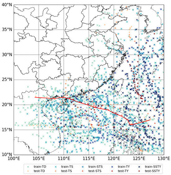
Figure 1.
TC point sample positions are denoted by “×” for model training and “+” for model testing. The colors of symbols “×” and “+”, ranging from light to dark, represent the TC intensity from weak to strong. The red line refers to the track of TC Ma-on.
This study uses cumulative precipitation with lead times of 6, 12, 18, 24, 30, 36, 42, 48, 54, 60, 66, and 72 h within a 20 × 20 degree region around the TC point locations as the predictands, which is provided by the Global Precipitation Measurement (GPM) Mission with a resolution of 0.25 degrees [40]. The predictors include real-time environmental background data and cumulative precipitation forecast data with the lead times within the 20 × 20 degree region around the TC point locations, which is provided by GFS [41]. Predictive modeling in this study is implemented using UNet-based neural networks.
GFS is an atmospheric circulation model developed and maintained by the National Oceanic and Atmospheric Administration (NOAA) of the United States. The GFS data have a spatial resolution of 0.25 degrees and a temporal resolution of 6 h. The TC point samples are selected from the best track dataset at 00, 06, 12, and 18 UTC to align with the daily GFS model forecast runs. To forecast the cumulative precipitation for a given time frame, the following steps are taken to process the GFS data for creating the input field of neural networks.
(1) Calculate the coordinate range of 10 latitudes and longitudes around the TC point based on its coordinates and time to select a 20 × 20 degree region whose center is the TC point location.
(2) Select cumulative precipitation forecast data corresponding to the specific lead time, and real-time environmental field data consisting of 24 atmospheric factors, based on the coordinate range. Table 2 displays the names and physical meanings of the cumulative precipitation forecast data and real-time environmental field data of 24 atmospheric factors, each with a data size of 80 × 80 (20 degree/0.25 degree resolution).
Table 2.
Variable names and their corresponding physical meanings.
(3) Integrate the data into a 25 × 80 × 80 array, constituting the neural network’s input field for a TC point with a specific lead time. Each input field for a TC point includes cumulative precipitation forecast data with a size of 80 × 80 and real-time environmental field data with a size of 24 × 80 × 80.
For instance, if the coordinates of a TC point are 120 E and 20 N at a particular moment, and the specific lead time for the predictand is 24 h, we use GFS real-time data corresponding to 24 atmospheric factors in the coordinate range of 110–130 E and 10–30 N at that moment. Additionally, we use the future 0–24 h GFS cumulative precipitation forecast data in the coordinate range of 110–130 E and 10–30 N. The real-time environmental field data and 24-h GFS cumulative precipitation forecast data are integrated into a 25 × 80 × 80 size.
The precipitation observation data provided by the GPM [40] have a resolution of 0.25 degrees. For a TC point, the predictand is an 80 × 80 single-channel image that includes the cumulative precipitation data of a 20 × 20 degree region surrounding the TC point location. The GPM is an international satellite mission jointly operated by the National Aeronautics and Space Administration (NASA) and the Japan Aerospace Exploration Agency (JAXA). It utilizes multi-sensor, multi-satellite, and multi-algorithm data, along with a satellite network and rain gauge inversion, to obtain highly accurate precipitation data. Using microwave and infrared technology, the GPM provides global rain and snow data products, including up to 3 h of microwave-based data and half-hourly microwave-infrared-based data [40,42]. As a result, it is frequently used as a source of precipitation observation data [42].
2.2. U-Net-Based Models
The U-Net and UNet3+ architectures, provided by Ronneberger et al. (2015) and Huang et al. (2020), respectively, form the basis of most of the neural network models described in this study (see Figure 2) [27,43]. The U-Net design comprises an encoder and a decoder. The encoder uses double convolution and max pooling operations to extract features, while the decoder uses the same layers for upsampling [29]. U-Net employs a pixel-to-pixel mapping technique between the input and output images. UNet3+ is an improved version of the U-Net model that utilizes full-scale jump connections to merge low-level information with high-level semantics from feature maps of varying sizes, thereby optimizing the usage of full-scale feature maps [35,36,37].
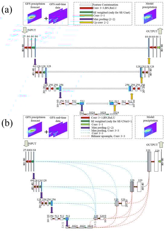
Figure 2.
Structures of (a) U-Net and SE-UNet and (b) UNet3+ and SE-UNet3+.
SE-UNet and SE-UNet3+ are U-Net and UNet3+ models that incorporate attention modulation. This modulation directs the network towards task-relevant aspects by suppressing feature responses in irrelevant settings [32,33]. Various attention strategies have been proposed to improve neural network performance [44,45]. In this study, we aim to improve precipitation prediction accuracy by incorporating Squeeze-and-Excitation (SE) modules into the U-Net family of networks. Figure 2 illustrates the incorporation of an SE module behind each encoder layer, resulting in the SE-UNet and SE-UNet3+ models. For comparison, the U-Net and UNet3+ models, lacking an SE module, are also used in this study. Additionally, we develop a neural network using the VGG16 architecture to compare the generalizability of neural networks with varying architectures. The structure of VGG is illustrated in Figure S1 (see Supplementary Materials for further details).
The neural network generates an 80 × 80 single-channel image, representing the cumulative precipitation forecast for various lead times. To assess the model’s performance against GPM precipitation observation, we use the mean square error between GPM observation and model precipitation forecast as the neural network’s loss function, as demonstrated in Formula (1).
where is the GPM precipitation observation and is the model precipitation forecast. The adaptive moment estimation (Adam) optimizer is used to optimize the network parameters [46].
2.3. Ensemble Method for TC Precipitation Forecasts
To comprehensively make use of the precipitation forecasts from different models, i.e., U-Net, UNet3+, SE-UNet, and SE-UNet3+, we use various ensemble methods to enhance the TC precipitation forecast accuracy. The TC precipitation forecast in this study can be considered a quantitative precipitation forecast (QPF). A simple ensemble strategy to improve QPF is to average over all members at each grid point to generate an overall mean (AVR) [47,48,49]. This mean value emphasizes the common qualities of individual members while significantly reducing the maximum intensity [50]. Additionally, several studies have demonstrated that the AVR greatly underestimates reported precipitation intensities while increasing the spatial coverage of drizzle [51,52,53].
Another ensemble method to improve QPF outcomes is the probability matching (PM) strategy. Ebert (2001) first applied this technique to QPF outcomes [52], assuming that the most likely spatial representation of the rain field is given by the AVR, while the best frequency distribution of rain rates is given by the ensemble of model QPFs. The PM approach has been frequently used to improve the performance of QPF ensembles, outperforming individual QPF members [54,55,56,57].
The following steps are followed for performing probabilistic matching:
(1) Compute the ensemble average at each grid point by taking the simple arithmetic average of all members.
(2) Record the rank and location of each value by sorting the ensemble mean values from lowest to highest.
(3) Sort the ensemble members’ values from lowest to highest and consider every n (n = number of members) values as a group.
(4) Select the groups from lowest to highest and insert the median of each group into the position where the mean set is sorted from lowest to highest. For example, substitute the grid point with the largest precipitation amount in the ensemble mean with the median of the highest n value in the ensemble member distribution.
2.4. Evaluation Metrics
The performance of the neural network is evaluated using the mean average error (MAE) (Formula (2)) and the root mean square error (RMSE) (Formula (3)) for TC precipitation on the test set. In Formulas (2) and (3), represents the GPM precipitation observation and represents the model precipitation forecast.
However, it is important to note that reducing the RMSE and MAE does not always result in an increase in the threat score (TS) [58], which is another commonly used metric for evaluating precipitation forecast skills. The TS objectively determines whether the intensity of precipitation will exceed a certain threshold and is calculated using the following formula:
where A represents the number of correct occurrence forecasts (hits), B represents the number of wrong occurrence forecasts (false alarms), and C represents the number of incorrect non-occurrence forecasts (misses). Different precipitation forecast thresholds correspond to different TS scores. In this study, we primarily evaluate the TS scores using precipitation thresholds of 10 mm/day, 25 mm/day, 50 mm/day, and 100 mm/day. Furthermore, we calculate the spatial correlation between the precipitation forecasts and observations to identify the precipitation forecast model that best matches the spatial distribution of precipitation forecasts to the observations.
TS = A/(A + B + C)
2.5. Feature Importance Analysis
A crucial aspect of evaluating a model is analyzing the importance of its features. This analysis enables us to identify elements that require optimization. To assess feature importance, we employ the permutation feature importance (PFI) approach [59]. In this study, we evaluate the impact of 25 input variables on model fitting by sequentially shuffling the variables in each of the 25 input channels and independently estimating the loss increase due to each shuffling. In this study, we examine the relative importance of 25 variables, calculated as the absolute importance divided by the sum of the absolute importance of all variables.
The absolute feature importance is calculated using the following steps:
(1) Denote the loss on the neural network test set without shuffling as loss1. Then, choose one variable and randomly disrupt the data in the neural network’s input field of the test set corresponding to the channel of that variable. Finally, feed it into the neural network to calculate the loss after disruption, which is denoted as loss2. To determine the increase in loss, calculate the difference between loss2 and loss1, denoted as loss3. This step is referred to as 1 permutation.
(2) Complete 500 permutations for this variable and calculate the mean value of the 500 loss3s. This mean value is referred to as the feature importance of this variable.
2.6. Case Study
We choose TC Ma-on, known for causing heavy precipitation [60,61], as a case study to evaluate the neural network’s performance in predicting precipitation. TC Ma-on made landfall at approximately 113 E, 20.5 N, with a central wind speed of 35 m/s at 18:00 on 24 August 2022. The analysis period spans from 00:00 on 21 August 2022, to 12:00 on 25 August 2022. During this period, we calculate the mean value of TC Ma-on’s GFS cumulative precipitation forecast, the neural network’s precipitation forecast, and observed precipitation. The track of TC Ma-on is denoted by the red line in Figure 1.
3. Results
The aim of this study is to utilize neural network models to predict TC precipitation in the Northwest Pacific region using real-time GFS data and GFS precipitation forecast data. The evaluation of the neural network’s effectiveness in forecasting TC precipitation is based on its performance on the test set, the TS score for predicting precipitation, the performance of the precipitation simulation for individual TC cases, and the feature importance. The following sections describe the results in detail.
3.1. Basic Performance
Figure 3 displays the RMSEs for various models at different lead times. The results indicate that the RMSE increases with longer lead times, potentially attributed to the increased uncertainty associated with longer forecasts. Specifically, the VGG model has the highest overall RMSE, followed by the GFS model. Notably, the median RMSEs of the two ensemble models, AVR and PM, are consistently the lowest at each lead time.
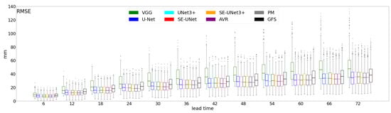
Figure 3.
Boxplots of RMSEs for different models with various lead times. The box plot shows the median (line inside the box) and the upper and lower quartiles (top and bottom of the box), while the whiskers extend to the minimum and maximum non-outlier values. Outliers are indicated by dots beyond the whiskers.
Figure 4 illustrates the mean RMSEs for various models used to forecast precipitation induced by TC points with varying intensities. The mean RMSEs of all TC points are presented in Figure 4a. The VGG model produces the highest average RMSE across all TC levels, followed by the GFS model. Figure 4b–f demonstrate that UNet-based models consistently produce lower RMSEs than GFS models at different TC levels. Specifically, the GFS models have mean RMSEs of 20.51 mm, 32.29 mm, and 41.07 mm at lead times of 24 h, 48 h, and 72 h, respectively. In contrast, the UNet-based models exhibit lower mean RMSEs at the same lead times: U-Net 19.25 mm, 29.65 mm, 37.78 mm; UNet3+ 18.61 mm, 29.10 mm, 37.30 mm; SE-UNet 18.31 mm, 29.11 mm, 37.93 mm; SE-UNet3+ 18.24 mm, 28.93 mm, 37.56 mm; AVR 18.17 mm, 28.74 mm, 36.87 mm; PM 18.16 mm, 28.72 mm, 36.84 mm. On average, the RMSEs of precipitation forecasts by U-Net, UNet3+, SE-UNet, SE-UNet3+, AVR, and PM are lower by 8.7%, 10.1%, 9.7%, 10.0%, 11.4%, and 11.5%, respectively, compared with the GFS model’s precipitation forecasts. This result suggests that the neural network model based on the U-Net structure effectively reduces the RMSE of precipitation predictions compared with the GFS model. Notably, the UNet3+, SE-UNet, and SE-UNet3+ models with improved U-Net structures reduce the RMSE more effectively than the standard U-Net model. Additionally, the ensemble models, AVR and PM, exhibit lower RMSE than any separate precipitation prediction models.
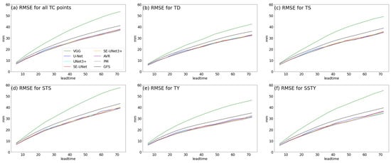
Figure 4.
RMSEs of different models for various TC levels: (a) all TC points, (b) TD, (c) TS, (d) STS, (e) TY, and (f) SSTY.
Based on Figure 4, the PM model has a lower average RMSE compared with other models, and therefore we use it for comparison with the GFS model. Figure 5 illustrates the spatial distribution of RMSEs for both PM and GFS models at different lead times. Comparing Figure 5a–c with Figure 5d–f, we observe that the high RMSE areas for both models are concentrated near the TC center, which may be associated with heavy precipitation in that area. The RMSEs for PM models at lead times of 24 h, 48 h, and 72 h are 18.16 mm, 28.72 mm, and 36.84 mm, respectively, lower than the RMSEs for GFS models at the same lead times, which are 20.51 mm, 32.29 mm, and 41.07 mm, respectively. Figure 5g–i illustrate the difference between the average RMSEs for PM and GFS models, consistently showing lower RMSEs for PM models in most regions. The average differences are 2.35 mm, 3.57 mm, and 4.33 mm at lead times of 24 h, 48 h, and 72 h, respectively, increasing with longer lead times. The higher RMSE difference between PM and GFS models near the TC center, as shown in Figure 5g–i, implies that the PM model primarily optimizes precipitation prediction RMSE in that area.
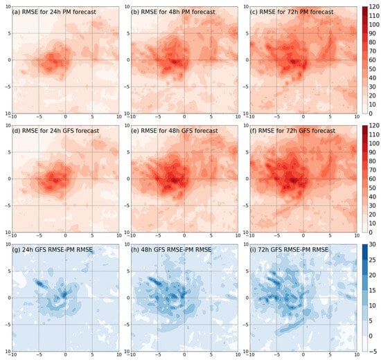
Figure 5.
The spatial distribution of precipitation prediction RMSE (mm) by PM and GFS models with different lead times: (a) PM with 24 h, (b) PM with 48 h, (c) PM with 72 h, (d) GFS with 24 h, (e) GFS with 48 h, (f) GFS with 72 h. The spatial distribution of the RMSE (mm) difference in precipitation prediction between GFS model and PM model with different lead times: (g) 24 h, (h) 48 h, and (i) 72 h.
Similar to the RMSE analysis, the MAE analysis (Figures S2 and S3 in the Supplementary Materials) reveals that the UNet-based models outperform the GFS model in reducing MAE. The PM models consistently exhibit the lowest average MAE compared with other models, aligning with the RMSE calculation results. The spatial distribution of MAE further emphasizes the PM model’s effectiveness in reducing MAE in precipitation prediction, particularly near the TC center.
Figure 6 illustrates the TSs for different models to forecast precipitation with different thresholds at various lead times, while Figure 7 displays the mean TS variations at different lead times. The figures demonstrate that the VGG model produces the lowest TSs for all thresholds, followed by the GFS model. There is a significant decrease in TSs for all models as the lead time increases, particularly at higher precipitation thresholds (50 mm/day and 100 mm/day) (Figure 6c,d and Figure 7c,d).
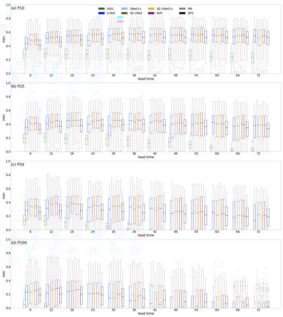
Figure 6.
Boxplots of TSs for precipitation prediction at different precipitation thresholds: (a) 10 mm/day, (b) 25 mm/day, (c) 50 mm/day, and (d) 100 mm/day.
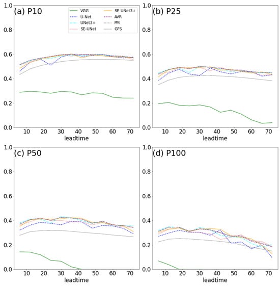
Figure 7.
TSs in precipitation prediction by different models with different lead times for various precipitation thresholds: (a) 10 mm/day, (b) 25 mm/day, (c) 50 mm/day, and (d) 100 mm/day.
Figure 7a shows that when the precipitation threshold is 10 mm/day, the mean TSs for GFS models are 0.52, 0.55, and 0.55 at lead times of 24 h, 48 h, and 72 h, respectively. These values are lower than most of the mean TSs for UNet-based models at the same lead times. Similarly, when the precipitation thresholds are 25 mm/day, 50 mm/day, and 100 mm/day, UNet-based models produce higher TSs than GFS models at most lead times. On average, the TS scores of U-Net, UNet3+, SE-UNet, SE-UNet3+, AVR, and PM are raised by 12.8%, 21.3%, 19.3%, 20.7%, 22.5%, and 22.9%, respectively, when compared with the GFS model. The models with improved U-Net structures, namely UNet3+, SE-UNet, and SE-UNet3+, show a more effective improvement in TS scores than the standard U-Net model. Meanwhile, the integrated models, AVR and PM, exhibit higher TS scores than any separate precipitation prediction models.
Overall, the neural network model used in this study performs well in reducing the RMSE and raising the TS of precipitation forecasts. In particular, the U-Net architecture represents an advancement in deep learning applications for precipitation forecasting [15]. This study further utilizes improved U-Net structures, such as UNet3+, SE-UNet, and SE-UNet3+, as well as an ensemble of outputs from all these models. Compared with the GFS model, the traditional U-Net model reduces the RMSE by 8.7% and improves the TS by 12.8% in precipitation forecasts. In contrast, our best ensemble model, the PM model, reduces the RMSE by 11.5% and improves the TS by 22.9% in precipitation forecasts.
3.2. Case Study
Figure 8 presents the MAEs and RMSEs of precipitation forecasts for TC Ma-on by the GFS and PM models at various lead times, indicating that the PM model exhibits lower values for both metrics compared with the GFS model. The average cumulative precipitation for the PM model forecast, GFS model forecast, and GPM observation over 0–24 h are 12.02 mm, 10.87 mm, and 12.76 mm, respectively, indicating that the PM model effectively corrects the GFS model’s precipitation underestimation within 0–24 h. Similarly, the average cumulative precipitation for the PM model forecast, GFS model forecast, and GPM observation over 0–48 h are 21.59 mm, 20.82 mm, and 21.88 mm, and over 0–72 h are 28.94 mm, 28.42 mm, and 28.83 mm, respectively. The PM model’s average precipitation forecast aligns more closely with GPM observation compared with the GFS model.
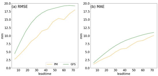
Figure 8.
(a) RMSE and (b) MAE for precipitation prediction for TC Ma-on by different models.
Additionally, we select a TC point where TC Ma-on caused the heaviest 0–24 accumulated precipitation before its landfall and analyze the spatial distribution pattern of forecasted and observed precipitation at that point. Figure 9 illustrates the TC precipitation forecasts by the PM and GFS models, along with the GPM precipitation observation, when TC Ma-on was located at 113 E, 20.5 N, causing heavy precipitation in Hainan province. The spatial correlations between the precipitation forecasts by the PM model and the GPM observations over 0–24 h, 0–48 h, and 0–72 h are 0.81, 0.80, and 0.78, respectively, higher than the spatial correlations between precipitation forecasts by the GFS model and the GPM observations, i.e., 0.71, 0.70, and 0.69, respectively. Precipitation forecasts by the PM model are more similar to the GPM precipitation observations in terms of precipitation distribution patterns, indicating an improvement over the GFS model in TC Ma-on precipitation forecasts.
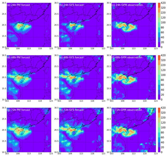
Figure 9.
Comparison between the accumulated precipitation forecasts (mm) by PM and GFS models with different lead times, and the precipitation observations by GPM for TC Ma-on at 113° E, 20.5° N: precipitation forecasts by PM with different lead times of (a) 24 h, (d) 48 h, (g) 72 h; precipitation forecasts by GFS with different lead times of (b) 24 h, (e) 48 h, (h) 72 h; accumulated precipitation observation by GPM within different periods of (c) 24 h, (f) 48 h, (i) 72 h. The red star denotes the TC Ma-on location.
3.3. Feature Importance Analysis
The feature importance analysis for U-Net, SE-UNet, UNet3+, and SE-UNet3+ models at lead times of 24 h, 48 h, and 72 h is presented in Figure 10 (showing only the ten most important features) for 24 h, and Figures S5 and S6 for 48 h and 72 h, respectively (see details in Supplementary Materials). The results suggest that the GFS precipitation forecast data is the most important variable among the 25 input variables, followed by the land and sea mask (lsm), which is a topography-related variable. Additionally, variables 500u and 500w are among the top ten most critical variables in each model at lead times of 24 h, 48 h, and 72 h, indicating the significance of the GFS precipitation forecast data, lsm, zonal wind speed at 500 hPa, and vertical speed at 500 hPa in the neural network training for the U-Net, SE-UNet, UNet3+, SE-UNet3+ models.
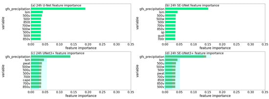
Figure 10.
The first 10 significant features for 24 h accumulated precipitation prediction by the models of (a) U-Net, (b) SE-UNet, (c) UNet3+, and (d) SE-UNet3+.
4. Conclusions
In this study, we employ UNet-based DL methods, including U-Net, UNet3+, SE-Net, and SE-UNet3+, to forecast TC precipitation in the Northwest Pacific region based on GFS precipitation forecast data and real-time GFS environmental background data. To maximize the utilization of the precipitation forecasts from these four DL models, we additionally employ two ensemble methods, PM and AVR, for rainfall prediction. GPM precipitation data are applied as the ground truth.
Compared with the GFS model, the RMSEs of UNet, UNet3+, SE-UNet, SE-UNet3+, AVR, and PM are lowered by 8.7%, 10.1%, 9.7%, 10.0%, 11.4%, and 11.5%, respectively, while the MAEs are reduced by 9.6%, 11.3%, 9.0%, 12.0%, 12.8%, and 13.0%. The TSs of the precipitation forecasts generated by these six models are higher than those of the GFS precipitation forecast, indicating that UNet-based models outperform the GFS model. Notably, the ensemble models, particularly PM, outperform all other individual models. By comparing the spatial distribution of RMSE and MAE for precipitation prediction by PM and GFS models, we find that the PM model can effectively improve the precipitation forecast accuracy near the TC center, where the GFS encounters significant precipitation forecast errors.
Furthermore, the feature importance analysis of U-Net, UNet3+, SE-UNet, and SE-UNet3+ reveals that the GFS precipitation forecast data are the most critical variable among the 25 input variables, followed by the l sm. Additionally, latitudinal wind speed at 500 hPa and vertical wind speed at 500 hPa are also important.
The study’s innovation lies in adopting the UNet3+ architecture, rarely explored in weather prediction research, and pioneering the application of probability matching techniques in TC precipitation forecasting. This hybrid approach, combining traditional numerical forecasting integration with DL methods, represents a significant advancement in TC precipitation prediction, offering novel insights and promising ways for future weather forecasting.
Supplementary Materials
The following supporting information can be downloaded at: https://www.mdpi.com/article/10.3390/w16050671/s1, Figure S1: VGG model structure; Figure S2: Boxplots of MAE for different models with various lead times; Figure S3: MAEs of different models for various TC levels; Figure S4: The spatial distribution of precipitation prediction MAE (mm) by PM and GFS models with different lead times; Figure S5: The first 10 significant features for 48-h accumulated precipitation prediction; Figure S6: The first 10 significant features for 72-h accumulated precipitation prediction.
Author Contributions
Conceptualization, L.H. and Q.L.; Data curation, L.H.; Formal analysis, L.H. and Q.L.; Funding acquisition, Q.L.; Investigation, L.H. and Q.L.; Methodology, L.H., Q.L. and J.Z.; Project administration, Q.L.; Resources, Q.L., L.H. and J.Z.; Software, L.H. and Q.L.; Supervision, Q.L.; Validation, L.H., Q.L. and J.Z.; Visualization, L.H.; Writing—original draft, L.H. and Q.L.; Writing—review and editing, Q.L., X.D., Z.W., Y.W., P.-W.C. and N.L. All authors have read and agreed to the published version of the manuscript.
Funding
This study was supported by the Shenzhen Municipal Committee of Science and Technology Innovation with Grants of JCYJ20210324101006016 and GJHZ20210705141403010.
Data Availability Statement
The CMA tropical cyclone best track dataset is available at https://tcdata.typhoon.org.cn/zjljsjj.html (accessed on 2 July 2023). The GFS data (National Centers for Environmental Prediction, National Weather Service, NOAA, U.S. Department of Commerce, 2015) are available at the website https://rda.ucar.edu/datasets/ds084.1/ (accessed on 10 July 2023). The GPM IMERG Final Run V06 half-hourly precipitation product is available at the website https://disc.gsfc.nasa.gov/datasets/GPM_3IMERGHH_06/summary?keywords=%22IMERG%20final%22 (accessed on 10 July 2023).
Conflicts of Interest
The authors declare no conflicts of interest.
References
- Ren, F.; Wang, Y.; Wang, X.; Li, W. Estimating tropical cyclone precipitation from station observations. Adv. Atmos. Sci. 2007, 24, 700–711. [Google Scholar] [CrossRef]
- Yao, D.; Song, X.; Yang, L.; Ma, Y. Contribution of Tropical Cyclones to Precipitation around Reclaimed Islands in the South China Sea. Water 2020, 12, 3108. [Google Scholar] [CrossRef]
- Cai, Y.; Zheng, F.; Yao, C.; Lu, Q.; Qin, W.; He, H.; Huang, C. Spatiotemporal Distributions and Related Large-Scale Environmental Conditions of Extreme Rainfall from Tropical Cyclones with Different Tracks and Seasons in Guangxi, South China: A Comparative Climatological Study. Atmosphere 2023, 14, 1277. [Google Scholar] [CrossRef]
- Maxwell, J.T.; Bregy, J.C.; Robeson, S.M.; Knapp, P.A.; Soulé, P.T.; Trouet, V. Recent increases in tropical cyclone precipitation extremes over the US east coast. Proc. Natl. Acad. Sci. USA 2021, 118, e2105636118. [Google Scholar] [CrossRef]
- Hamill, T.M. Hypothesis tests for evaluating numerical precipitation forecasts. Weather Forecast. 1999, 14, 155–167. [Google Scholar] [CrossRef]
- Lin, C.; Vasić, S.; Kilambi, A.; Turner, B.; Zawadzki, I. Precipitation forecast skill of numerical weather prediction models and radar nowcasts. Geophys. Res. Lett. 2005, 32. [Google Scholar] [CrossRef]
- Zhang, P.; Zhang, L.; Leung, H.; Wang, J. A deep-learning based precipitation forecasting approach using multiple environmental factors. In Proceedings of the 2017 IEEE International Congress on Big Data (BigData Congress), Honolulu, HI, USA, 25–30 June 2017; pp. 193–200. [Google Scholar]
- Zhou, Y.; Lau, K.M.; Reale, O.; Rosenberg, R. AIRS impact on precipitation analysis and forecast of tropical cyclones in a global data assimilation and forecast system. Geophys. Res. Lett. 2010, 37, L02806. [Google Scholar] [CrossRef]
- Chen, Y.; Ebert, E.E.; Davidson, N.E.; Walsh, K.J. Application of contiguous rain area (CRA) methods to tropical cyclone rainfall forecast verification. Earth Space Sci. 2018, 5, 736–752. [Google Scholar] [CrossRef]
- Ray, K.; Balachandran, S.; Dash, S. Challenges of forecasting rainfall associated with tropical cyclones in India. Meteorol. Atmos. Phys. 2022, 134, 8. [Google Scholar] [CrossRef]
- Newman, K.M.; Brown, B.; Gotway, J.H.; Bernardet, L.; Biswas, M.; Jensen, T.; Nance, L. Advancing Tropical Cyclone Precipitation Forecast Verification Methods and Tools. Weather Forecast. 2023, 38, 1589–1603. [Google Scholar] [CrossRef]
- Huang, C.-L.; Hsu, N.-S.; Wei, C.-C.; Lo, C.-W. Using artificial intelligence to retrieve the optimal parameters and structures of adaptive network-based fuzzy inference system for typhoon precipitation forecast modeling. Adv. Meteorol. 2015, 2015, 472523. [Google Scholar] [CrossRef]
- Han, Y.; Zhang, G.J.; Huang, X.; Wang, Y. A moist physics parameterization based on deep learning. J. Adv. Model. Earth Syst. 2020, 12, e2020MS002076. [Google Scholar] [CrossRef]
- Reichstein, M.; Camps-Valls, G.; Stevens, B.; Jung, M.; Denzler, J.; Carvalhais, N.; Prabhat, f. Deep learning and process understanding for data-driven Earth system science. Nature 2019, 566, 195–204. [Google Scholar] [CrossRef]
- Sun, D.; Huang, W.; Yang, Z.; Luo, Y.; Luo, J.; Wright, J.S.; Fu, H.; Wang, B. Deep learning improves GFS wintertime precipitation forecast over southeastern China. Geophys. Res. Lett. 2023, 50, e2023GL104406. [Google Scholar] [CrossRef]
- Hu, Y.F.; Yin, F.K.; Zhang, W.M. Deep learning-based precipitation bias correction approach for Yin–He global spectral model. Meteorol. Appl. 2021, 28, e2032. [Google Scholar] [CrossRef]
- Wang, X.; Wang, W.; Yan, B. Tropical Cyclone Intensity Change Prediction Based on Surrounding Environmental Conditions with Deep Learning. Water 2020, 12, 2685. [Google Scholar] [CrossRef]
- Marchok, T.; Rogers, R.; Tuleya, R. Validation schemes for tropical cyclone quantitative precipitation forecasts: Evaluation of operational models for US landfalling cases. Weather Forecast. 2007, 22, 726–746. [Google Scholar] [CrossRef]
- Feng, Z.; Lv, S.; Sun, Y.; Feng, X.; Zhai, P.; Lin, Y.; Shen, Y.; Zhong, W. Skillful Seasonal Prediction of Typhoon Track Density Using Deep Learning. Remote Sens. 2023, 15, 1797. [Google Scholar] [CrossRef]
- Pradhan, R.; Aygun, R.S.; Maskey, M.; Ramachandran, R.; Cecil, D.J. Tropical cyclone intensity estimation using a deep convolutional neural network. IEEE Trans. Image Process. 2017, 27, 692–702. [Google Scholar] [CrossRef] [PubMed]
- Chen, R.; Zhang, W.; Wang, X. Machine learning in tropical cyclone forecast modeling: A review. Atmosphere 2020, 11, 676. [Google Scholar] [CrossRef]
- Wang, Z.; Zhao, J.; Huang, H.; Wang, X. A review on the application of machine learning methods in tropical cyclone forecasting. Front. Earth Sci. 2022, 10, 902596. [Google Scholar] [CrossRef]
- Gao, Y.; Guan, J.; Zhang, F.; Wang, X.; Long, Z. Attention-unet-based near-real-time precipitation estimation from fengyun-4A satellite imageries. Remote Sens. 2022, 14, 2925. [Google Scholar] [CrossRef]
- Kaparakis, C.; Mehrkanoon, S. WF-UNet: Weather Fusion UNet for Precipitation Nowcasting. arXiv 2023, arXiv:2302.04102. [Google Scholar]
- Trebing, K.; Staǹczyk, T.; Mehrkanoon, S. SmaAt-UNet: Precipitation nowcasting using a small attention-UNet architecture. Pattern Recognit. Lett. 2021, 145, 178–186. [Google Scholar] [CrossRef]
- Rasp, S.; Lerch, S. Neural networks for postprocessing ensemble weather forecasts. Mon. Weather Rev. 2018, 146, 3885–3900. [Google Scholar] [CrossRef]
- Ronneberger, O.; Fischer, P.; Brox, T. U-net: Convolutional networks for biomedical image segmentation. In Proceedings of the Medical Image Computing and Computer-Assisted Intervention–MICCAI 2015: 18th International Conference, Munich, Germany, 5–9 October 2015; pp. 234–241. [Google Scholar]
- Rozas Larraondo, P.; Renzullo, L.J.; Inza, I.; Lozano, J.A. A data-driven approach to precipitation parameterizations using convolutional encoder-decoder neural networks. arXiv 2019, arXiv:1903.10274. [Google Scholar]
- Dupuy, F.; Mestre, O.; Serrurier, M.; Burdá, V.K.; Zamo, M.; Cabrera-Gutiérrez, N.C.; Bakkay, M.C.; Jouhaud, J.-C.; Mader, M.-A.; Oller, G. ARPEGE cloud cover forecast postprocessing with convolutional neural network. Weather Forecast. 2021, 36, 567–586. [Google Scholar] [CrossRef]
- Singh, M.; Kumar, B.; Rao, S.; Gill, S.S.; Chattopadhyay, R.; Nanjundiah, R.S.; Niyogi, D. Deep learning for improved global precipitation in numerical weather prediction systems. arXiv 2021, arXiv:2106.12045. [Google Scholar]
- Honghan, Z.; Liu, D.C.; Jingyan, L.; Liu, P.; Yin, H.; Peng, Y. RMS-SE-UNet: A segmentation method for tumors in breast ultrasound images. In Proceedings of the 2021 IEEE 6th International Conference on Computer and Communication Systems (ICCCS), Chengdu, China, 23–26 April 2021; pp. 328–334. [Google Scholar]
- Liu, H.; Luo, J.; Huang, B.; Yang, H.; Hu, X.; Xu, N.; Xia, L. Building extraction based on SE-Unet. J. Geo-Inf. Sci. 2019, 21, 1779–1789. [Google Scholar]
- Sofla, R.A.D.; Alipour-Fard, T.; Arefi, H. Road extraction from satellite and aerial image using SE-Unet. J. Appl. Remote Sens. 2021, 15, 014512. [Google Scholar] [CrossRef]
- Zhang, G.; Yan, H.; Zhang, D.; Zhang, H.; Cheng, T.; Hu, G.; Shen, S.; Xu, H. Enhancing model performance in detecting lodging areas in wheat fields using UAV RGB Imagery: Considering spatial and temporal variations. Comput. Electron. Agric. 2023, 214, 108297. [Google Scholar] [CrossRef]
- Lv, M.; Zhang, Y.; Liu, S. Fast forward approximation and multitask inversion of gravity anomaly based on UNet3+. Geophys. J. Int. 2023, 234, 972–984. [Google Scholar] [CrossRef]
- Ono, S.; Komatsu, M.; Sakai, A.; Arima, H.; Ochida, M.; Aoyama, R.; Yasutomi, S.; Asada, K.; Kaneko, S.; Sasano, T. Automated endocardial border detection and left ventricular functional assessment in echocardiography using deep learning. Biomedicines 2022, 10, 1082. [Google Scholar] [CrossRef]
- Yin, M.; Wang, P.; Ni, C.; Hao, W. Cloud and snow detection of remote sensing images based on improved Unet3+. Sci. Rep. 2022, 12, 14415. [Google Scholar] [CrossRef] [PubMed]
- Lu, X.; Yu, H.; Ying, M.; Zhao, B.; Zhang, S.; Lin, L.; Bai, L.; Wan, R. Western North Pacific tropical cyclone database created by the China Meteorological Administration. Adv. Atmos. Sci. 2021, 38, 690–699. [Google Scholar] [CrossRef]
- Li, Q.; Xu, P.; Wang, X.; Lan, H.; Cao, C.; Li, G.; Zhang, L.; Sun, L. An operational statistical scheme for tropical cyclone induced wind gust forecasts. Weather Forecast. 2016, 31, 1817–1832. [Google Scholar] [CrossRef]
- Huffman, G.J.; Bolvin, D.T.; Braithwaite, D.; Hsu, K.; Joyce, R.; Xie, P.; Yoo, S.-H. NASA global precipitation measurement (GPM) integrated multi-satellite retrievals for GPM (IMERG). Algorithm Theor. Basis Doc. (ATBD) Version 2015, 4, 30. [Google Scholar]
- NCEP GFS 0.25 Degree Global Forecast Grids Historical Archive. Available online: https://rda.ucar.edu/datasets/ds084.1/dataaccess/ (accessed on 12 September 2023).
- Pradhan, R.K.; Markonis, Y.; Godoy, M.R.V.; Villalba-Pradas, A.; Andreadis, K.M.; Nikolopoulos, E.I.; Papalexiou, S.M.; Rahim, A.; Tapiador, F.J.; Hanel, M. Review of GPM IMERG performance: A global perspective. Remote Sens. Environ. 2022, 268, 112754. [Google Scholar] [CrossRef]
- Huang, H.; Lin, L.; Tong, R.; Hu, H.; Zhang, Q.; Iwamoto, Y.; Han, X.; Chen, Y.-W.; Wu, J. Unet 3+: A full-scale connected unet for medical image segmentation. In Proceedings of the ICASSP 2020—2020 IEEE International Conference on Acoustics, Speech and Signal Processing (ICASSP), Barcelona, Spain, 4–8 May 2020; pp. 1055–1059. [Google Scholar]
- Varshaneya, V.; Balasubramanian, S.; Gera, D. Res-SE-Net: Boosting Performance of ResNets by Enhancing Bridge Connections. In Machine Learning Algorithms and Applications; Wiley: Hoboken, NJ, USA, 2021; pp. 61–75. [Google Scholar]
- Yu, X.; Jin, F.; Luo, H.; Lei, Q.; Wu, Y. Gross tumor volume segmentation for stage III NSCLC radiotherapy using 3D ResSE-Unet. Technol. Cancer Res. Treat. 2022, 21, 15330338221090847. [Google Scholar] [CrossRef]
- Kingma, D.P.; Ba, J. Adam: A method for stochastic optimization. arXiv 2014, arXiv:1412.6980. [Google Scholar]
- Leith, C.E. Theoretical skill of Monte Carlo forecasts. Mon. Weather Rev. 1974, 102, 409–418. [Google Scholar] [CrossRef]
- Murphy, A.H. Skill scores based on the mean square error and their relationships to the correlation coefficient. Mon. Weather Rev. 1988, 116, 2417–2424. [Google Scholar] [CrossRef]
- Speer, M.; Leslie, L. An example of the utility of ensemble rainfall forecasting. Aust. Meteorol. Mag. 1997, 46, 75–78. [Google Scholar]
- Warner, T.T. Numerical Weather and Climate Prediction; Cambridge University Press: Cambridge, UK, 2010. [Google Scholar]
- Clark, A.J.; Gallus, W.A.; Chen, T.-C. Contributions of mixed physics versus perturbed initial/lateral boundary conditions to ensemble-based precipitation forecast skill. Mon. Weather Rev. 2008, 136, 2140–2156. [Google Scholar] [CrossRef]
- Ebert, E.E. Ability of a poor man’s ensemble to predict the probability and distribution of precipitation. Mon. Weather Rev. 2001, 129, 2461–2480. [Google Scholar] [CrossRef]
- Hamill, T.M.; Engle, E.; Myrick, D.; Peroutka, M.; Finan, C.; Scheuerer, M. The US National Blend of Models for statistical postprocessing of probability of precipitation and deterministic precipitation amount. Mon. Weather Rev. 2017, 145, 3441–3463. [Google Scholar] [CrossRef]
- Berenguer, M.; Surcel, M.; Zawadzki, I.; Xue, M.; Kong, F. The diurnal cycle of precipitation from continental radar mosaics and numerical weather prediction models. Part II: Intercomparison among numerical models and with nowcasting. Mon. Weather Rev. 2012, 140, 2689–2705. [Google Scholar] [CrossRef]
- Clark, A.J.; Gallus, W.A.; Xue, M.; Kong, F. A comparison of precipitation forecast skill between small convection-allowing and large convection-parameterizing ensembles. Weather Forecast. 2009, 24, 1121–1140. [Google Scholar] [CrossRef]
- Novak, D.R.; Bailey, C.; Brill, K.F.; Burke, P.; Hogsett, W.A.; Rausch, R.; Schichtel, M. Precipitation and temperature forecast performance at the Weather Prediction Center. Weather Forecast. 2014, 29, 489–504. [Google Scholar] [CrossRef]
- Xue, M.; Kong, F.; Tomas, K.; Wang, Y.; Brewster, K.; Gao, J.; Wang, X.; Weiss, S.; Clark, A.; Kain, J. Realtime convection-permitting ensemble and convection-resolving deterministic forecasts of CAPS for the Hazardous Weather Testbed 2010 Spring Experiment. In Proceedings of the 24th Conference on Weather and Forecasting/20th Conference on Numerical Weather Prediction, Seattle, WA, USA, 23–27 January 2011. [Google Scholar]
- Donaldson, R.; Dyer, R.M.; Kraus, M.J. An objective evaluator of techniques for predicting severe weather events. In Proceedings of the Ninth Conference on Severe Local Storms, Norman, OK, USA, 21–23 October 1975. [Google Scholar]
- Fisher, A.; Rudin, C.; Dominici, F. All Models are Wrong, but Many are Useful: Learning a Variable’s Importance by Studying an Entire Class of Prediction Models Simultaneously. J. Mach. Learn. Res. 2019, 20, 1–81. [Google Scholar]
- Mitamura, M. Rainfall Characteristics of Severe Tropical Storm Talas and Topographical and Geological Features of the Kii Peninsula. In Intensified Sediment Disasters in Japan; CRC Press: Boca Raton, FL, USA, 2023; pp. 34–52. [Google Scholar]
- Shen, W.; Jin, Y.; Cong, P.; Li, G. Dynamic Coupling Model of Water Environment of Urban Water Network in Pearl River Delta Driven by Typhoon Rain Events. Water 2023, 15, 1084. [Google Scholar] [CrossRef]
Disclaimer/Publisher’s Note: The statements, opinions and data contained in all publications are solely those of the individual author(s) and contributor(s) and not of MDPI and/or the editor(s). MDPI and/or the editor(s) disclaim responsibility for any injury to people or property resulting from any ideas, methods, instructions or products referred to in the content. |
© 2024 by the authors. Licensee MDPI, Basel, Switzerland. This article is an open access article distributed under the terms and conditions of the Creative Commons Attribution (CC BY) license (https://creativecommons.org/licenses/by/4.0/).