

A Transfer Learning Approach Based on Radar Rainfall for River Water-Level Prediction


Abstract
1. Introduction
- Using the proposed CNN-LSTM model (without transfer learning), it is shown that water-level prediction using radar rainfall images is almost as accurate as using measurements from upstream hydrological stations in a torrential rainfall scenario in a relatively steep river in Japan.
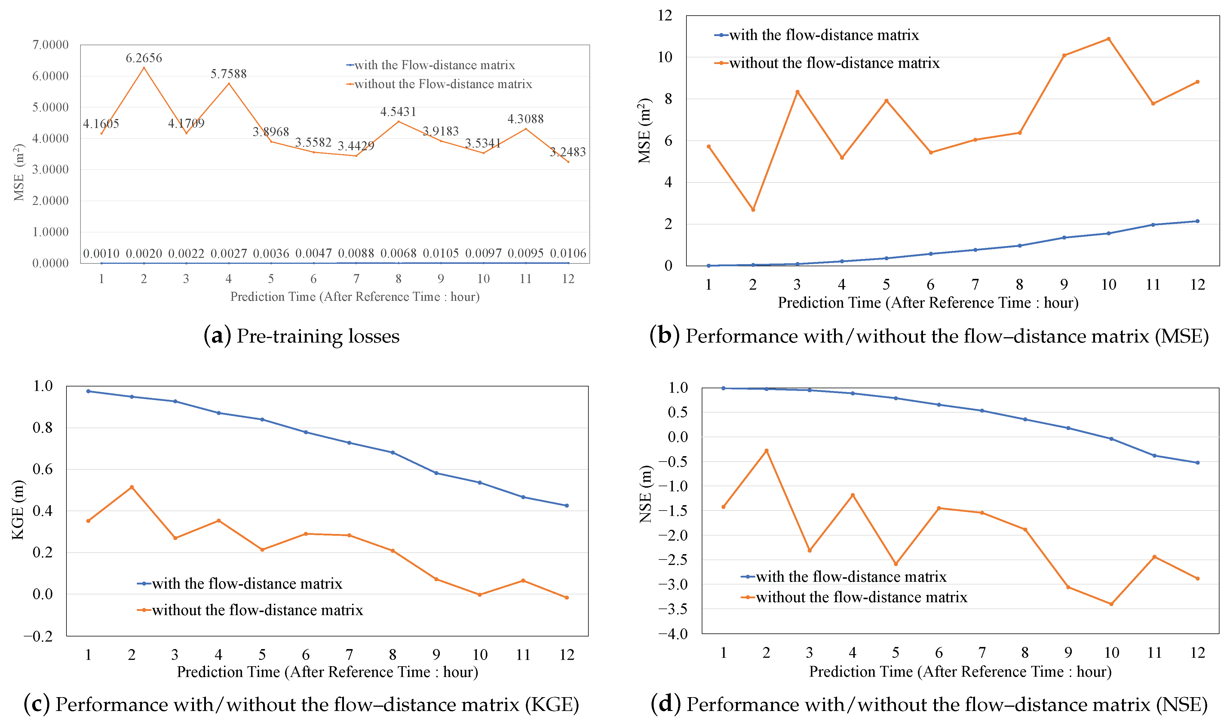
- By introducing the flow–distance matrix into transfer learning and using radar rainfall data from other river basins, we demonstrate that water levels can be predicted several hours in advance with high accuracy.
- Through these two contributions, we show fundamental results indicating that water level prediction would be feasible for medium and small rivers, for which historical flood measurements at the prediction site are scarce.
2. Materials and Methods
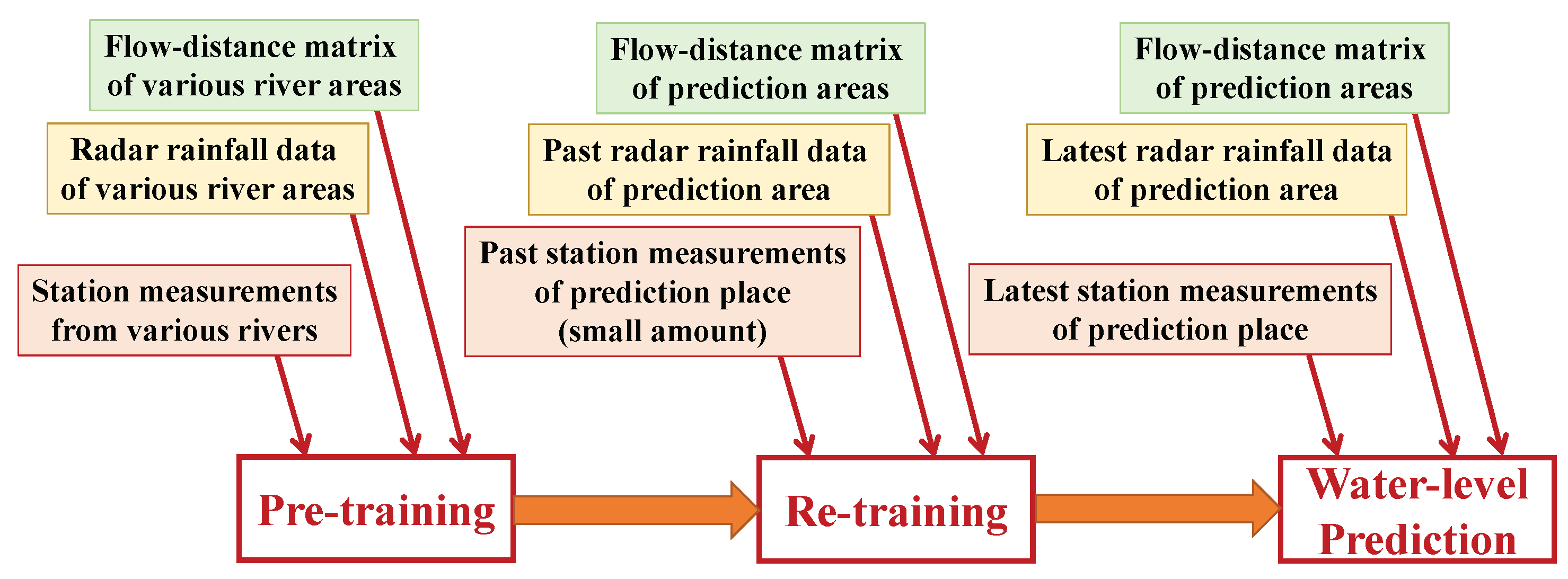
2.1. Overview
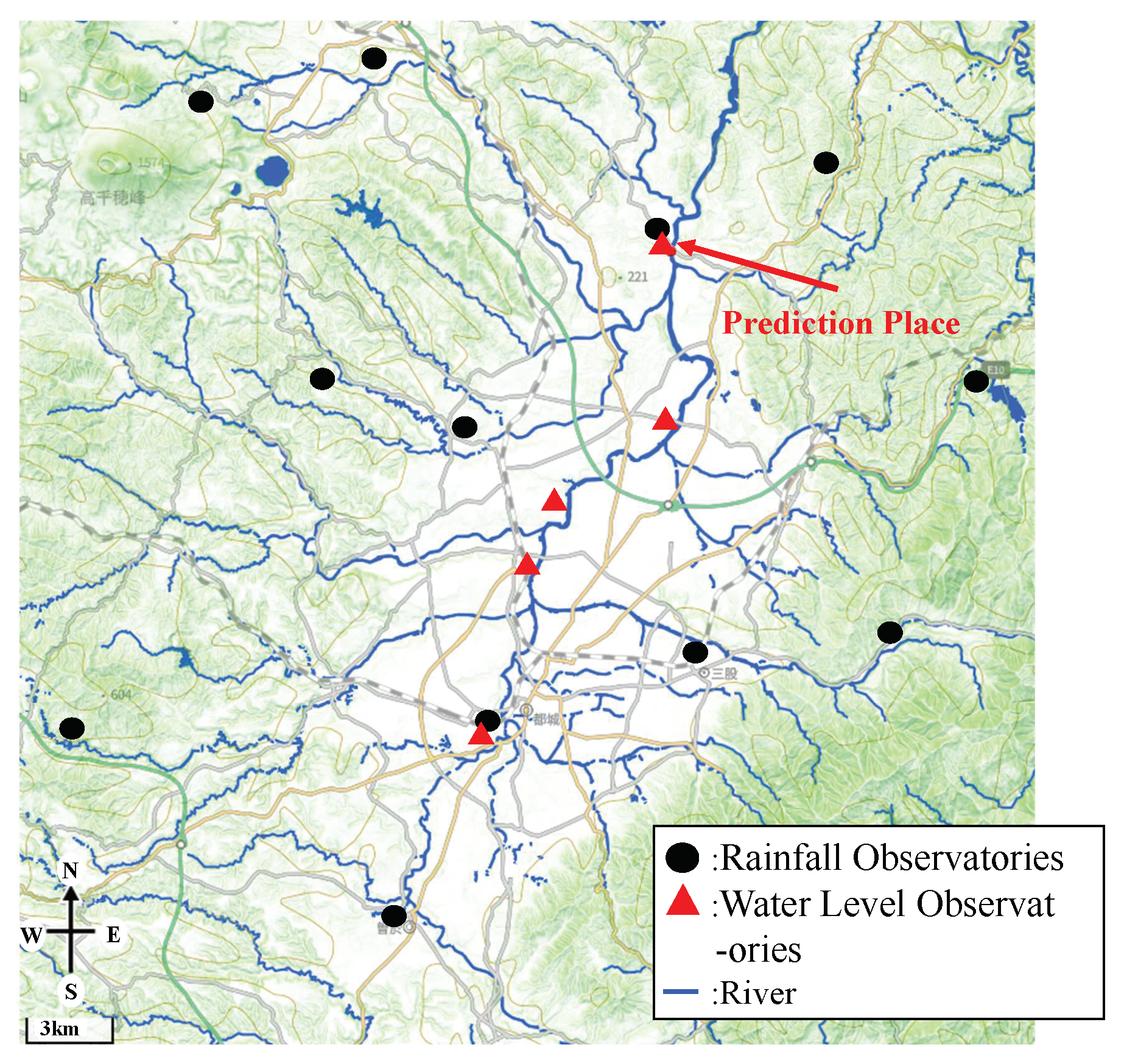
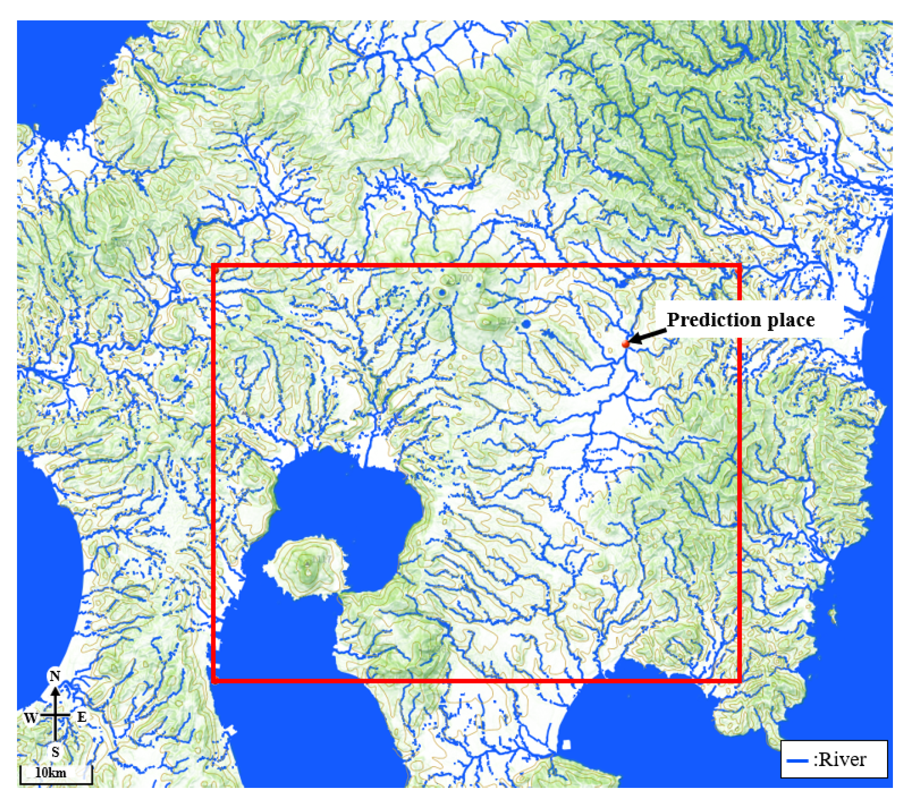
2.2. Study Area
2.3. Data Acquisition
2.4. Creating the Flow–Distance Matrix
2.5. Utilized Deep Learning Techniques
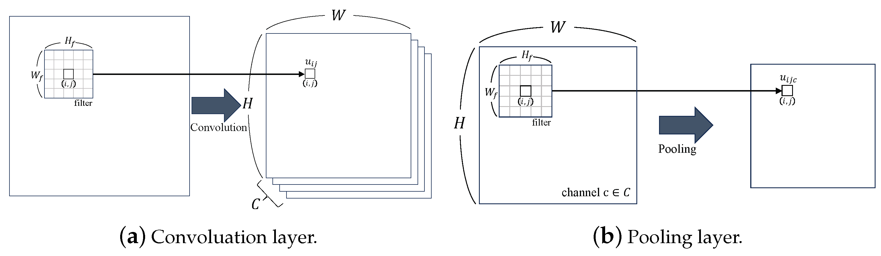
2.5.1. Convolutional Neural Network (CNN)
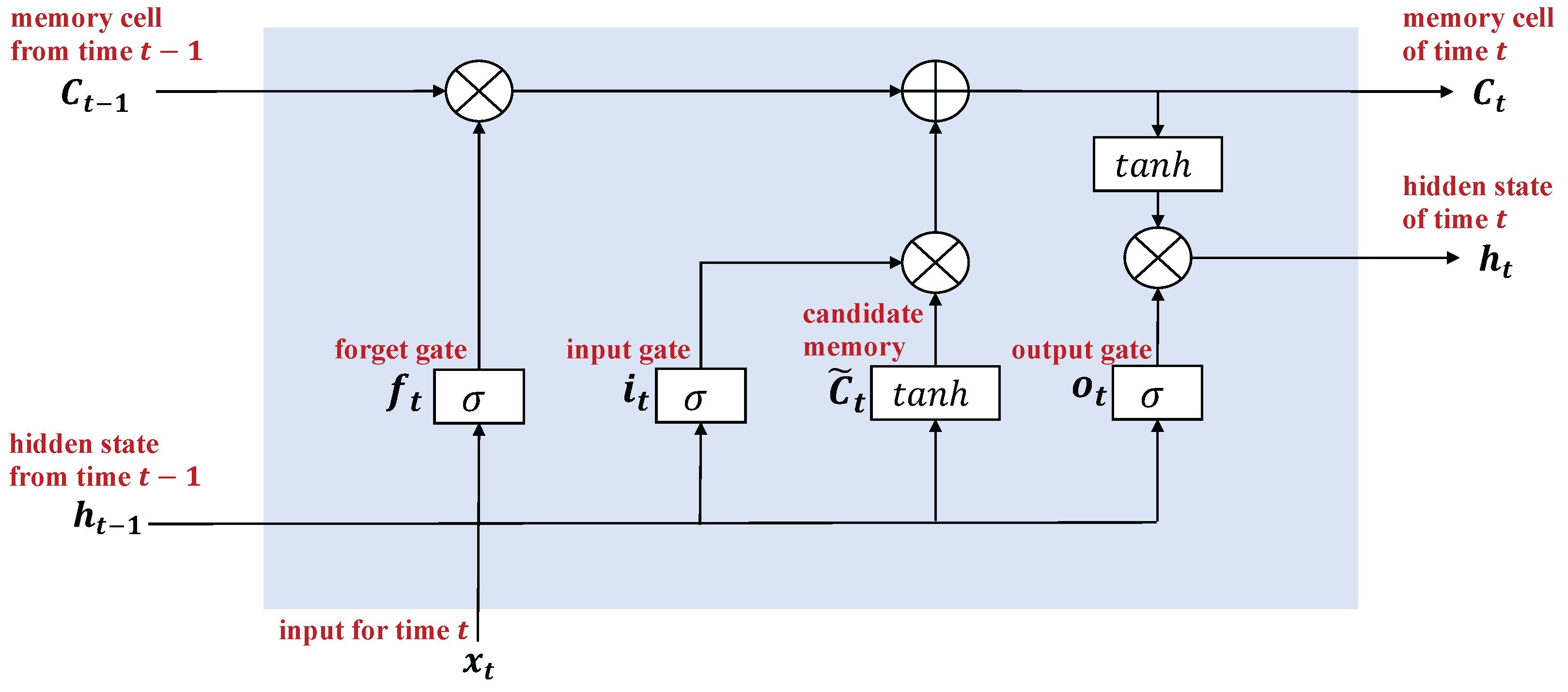
2.5.2. Long Short-Term Memory (LSTM)
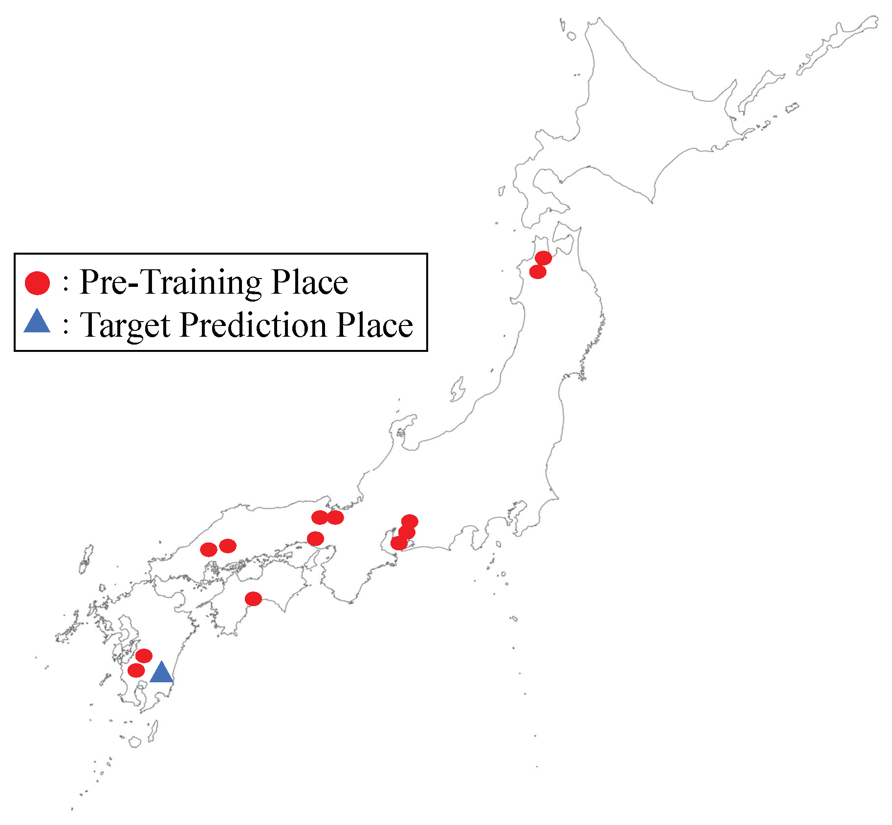
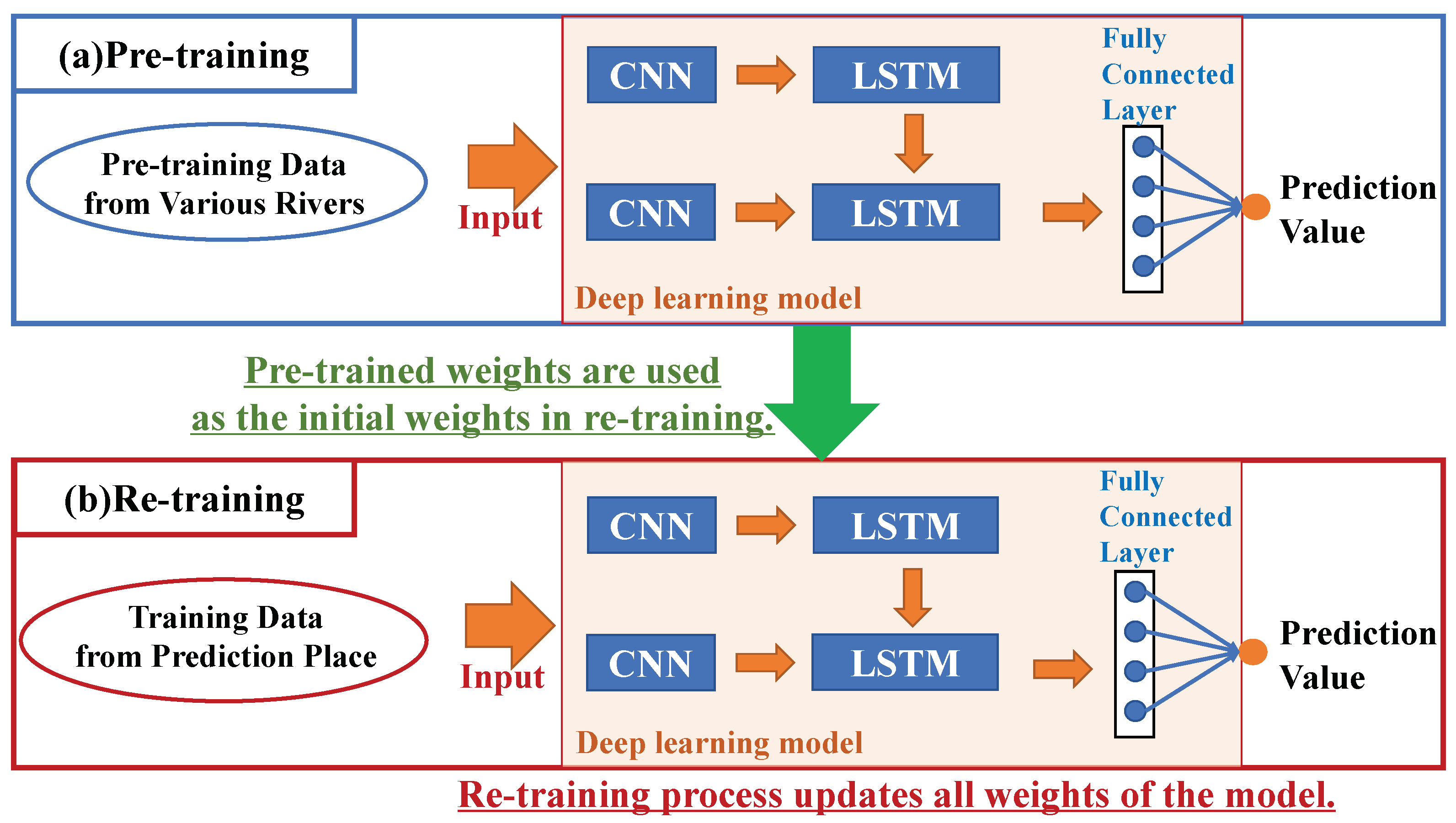
2.5.3. Transfer Learning
2.6. River Water-Level Prediction Model
2.6.1. The Basic Structure Combined with a CNN and LSTM
2.6.2. Our Transfer Learning Operations
2.6.3. The Parameter Details

| Item | Parameters |
|---|---|
| Optimizer | Pre-training: Adam [51] (0.0001) |
| Re-training: AdamW (0.00001) | |
| Epoch | Pre-training: 2000 |
| Re-training: Early stopping (50) | |
| Error function | MSE (Mean Squared Error) |
| Batch size | Pre-trianing: 90 |
| Re-training: 50 | |
| Language | Python version 3.9.12 |
| Library | PyTorch version 1.12.1 |
3. Results
3.1. Dataset
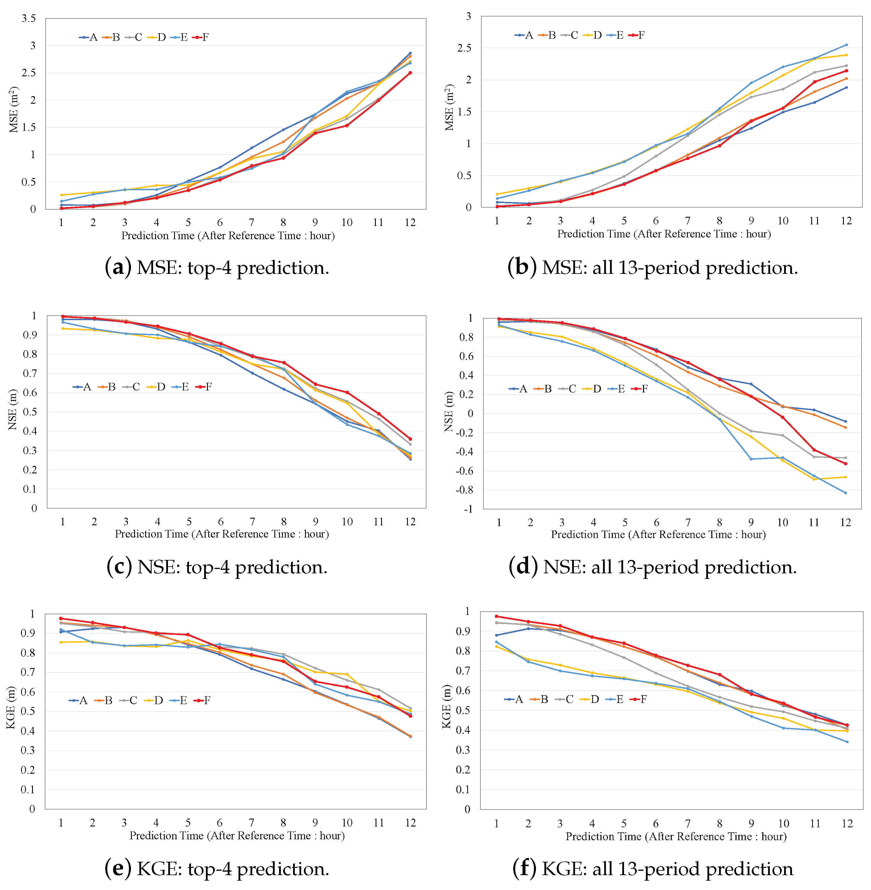
3.2. Evaluation Methods
- MLP with the upstream measurement data and the water-level + rainfall data at the prediction location (i.e., Hiwatashi).
- LSTM with the upstream measurement data and the water-level + rainfall data at the prediction location.
- CNN+LSTM with the radar rainfall data, the upstream measurement data, and the water-level + rainfall data at the prediction location.
- CNN+LSTM with the radar rainfall data and the water-level data at the prediction location.
- CNN+LSTM with the radar rainfall data, the water-level data at the prediction location, and the flow–distance matrix.
- CNN+LSTM, incorporating transfer learning with the radar rainfall data, water-level data at the prediction location, and the flow–distance matrix.
3.3. Parameter Selection
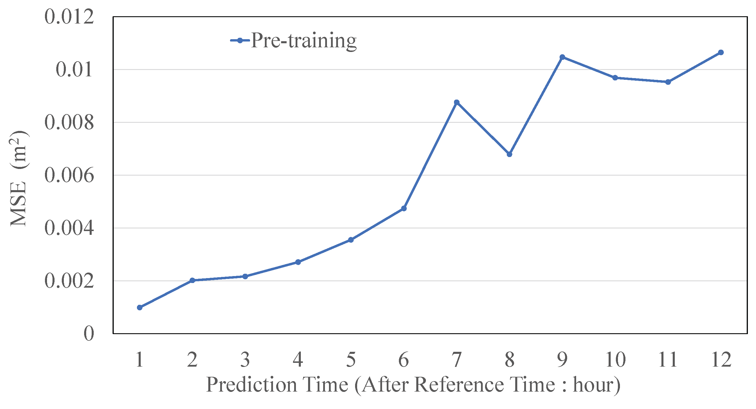
3.4. Performance in Pre-Training
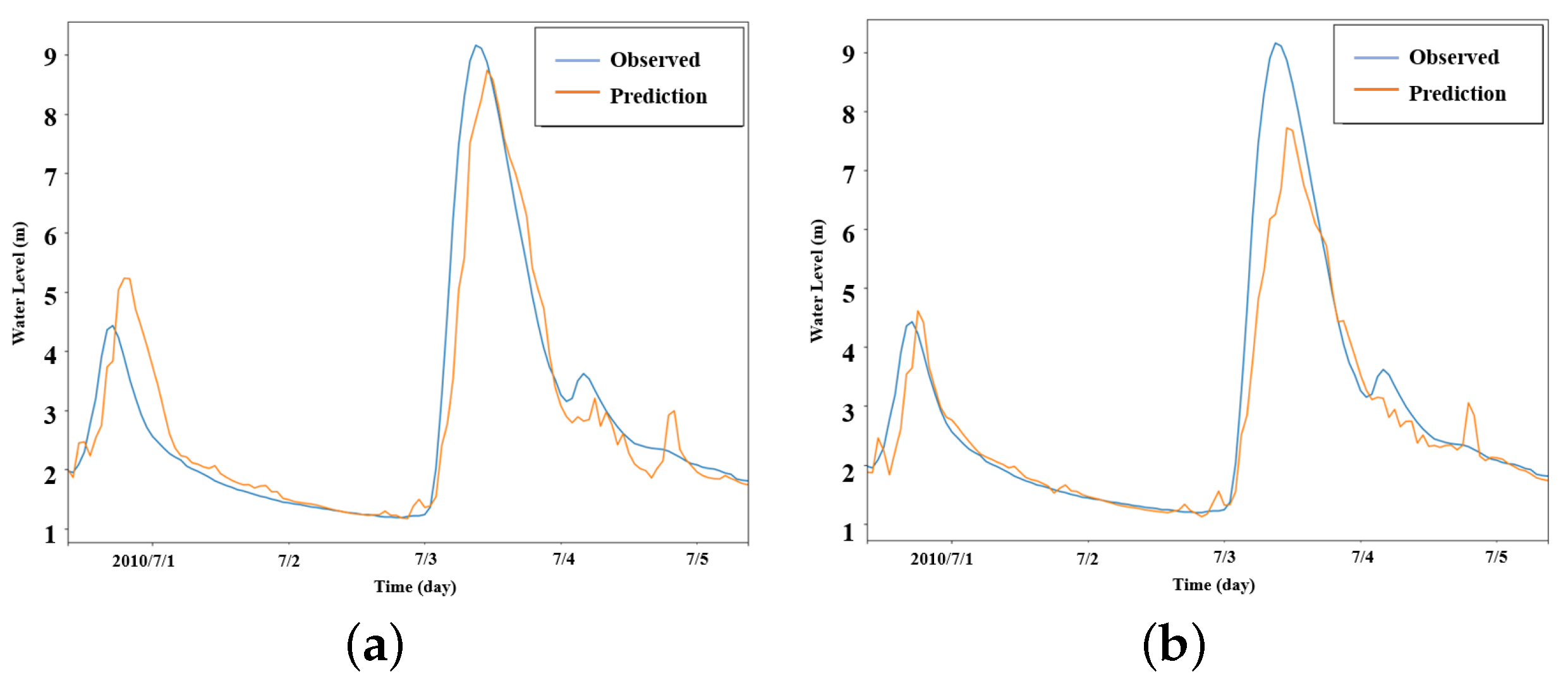
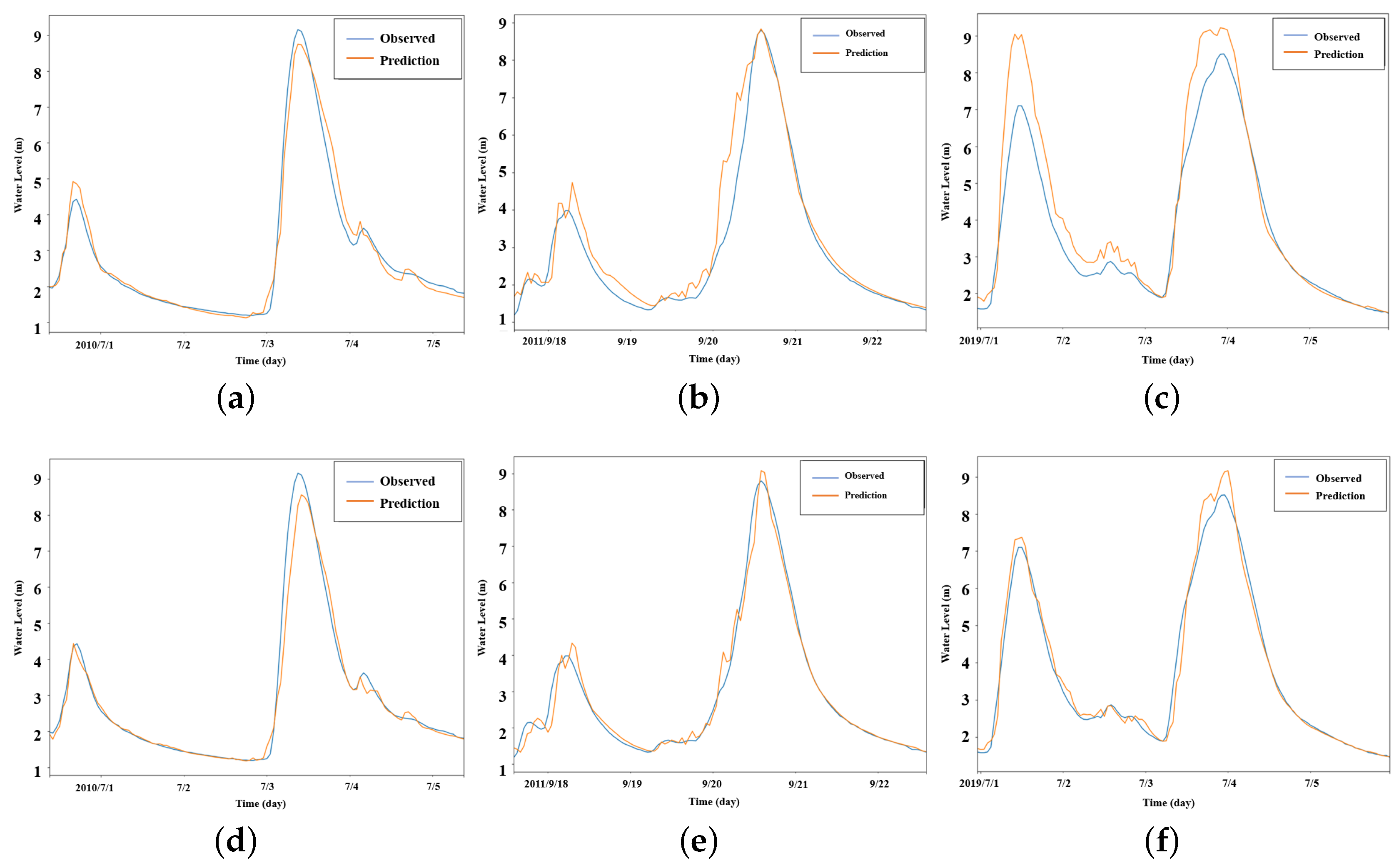
3.5. Performance of the Proposed Method
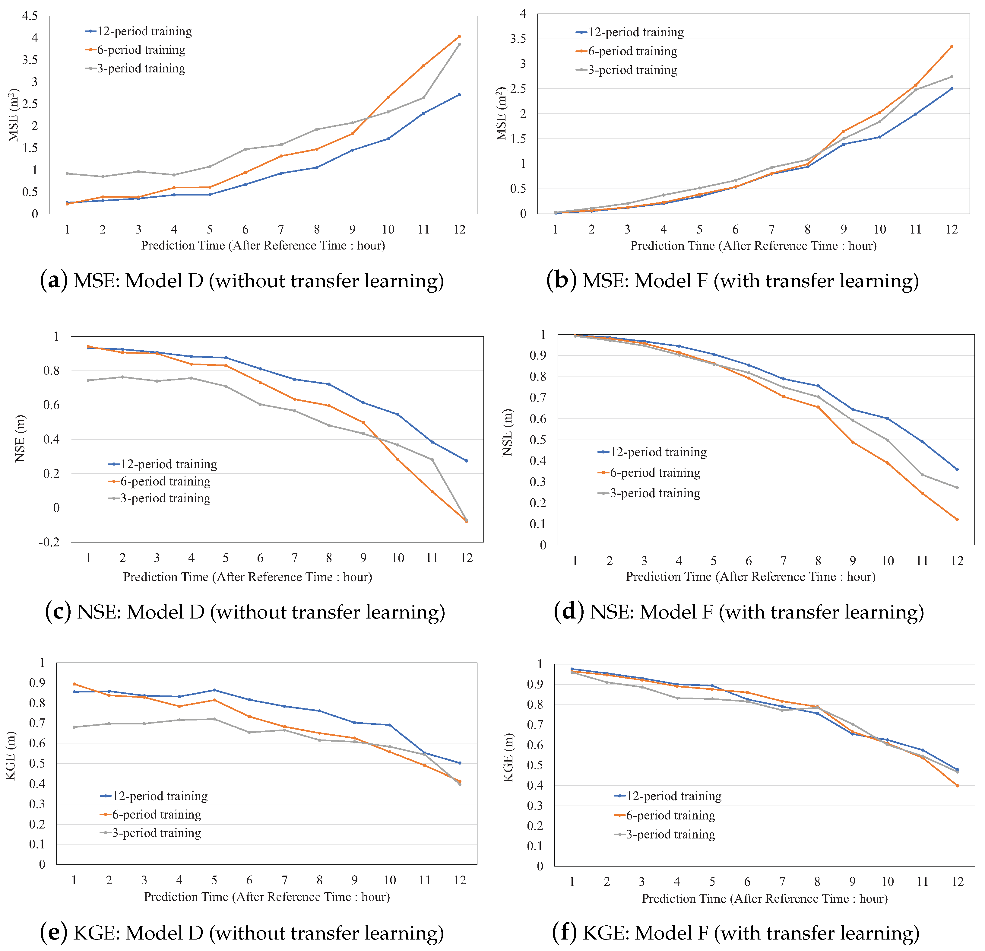
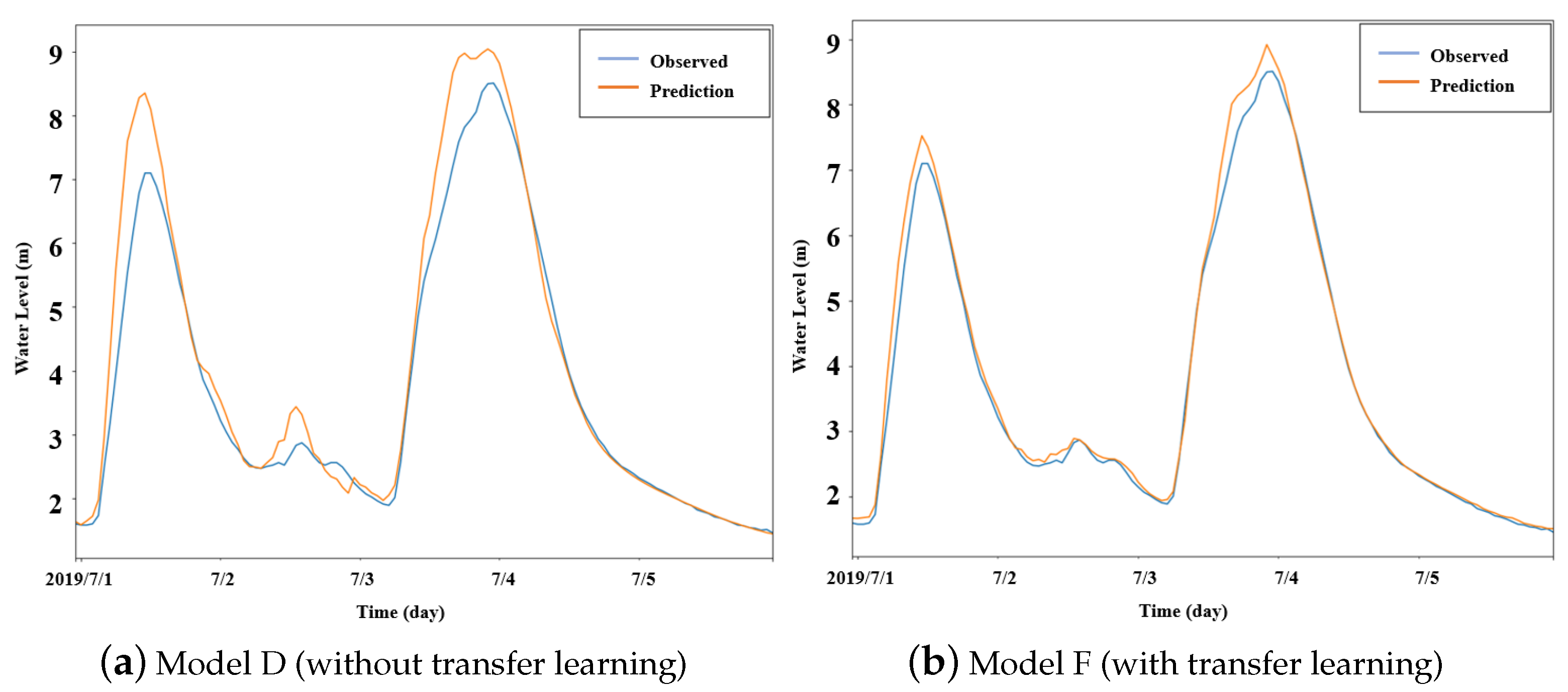
3.6. The Effect of Data Shortage
4. Discussion
5. Conclusions
Author Contributions
Funding
Data Availability Statement
Conflicts of Interest
References
- Kumar, V.; Sharma, K.V.; Caloiero, T.; Mehta, D.J.; Singh, K. Comprehensive Overview of Flood Modeling Approaches: A Review of Recent Advances. Hydrology 2023, 10, 141. [Google Scholar] [CrossRef]
- Asian Disaster Reduction Center. Natural Disaster Data Book 2022 (An Analytical Overview). Available online: https://reliefweb.int/report/world/natural-disaster-data-book-2022-analytical-overview (accessed on 26 December 2023).
- Nihei, Y.; Oota, K.; Kawase, H.; Sayama, T.; Nakakita, T.; Ito, T.; Kashiwada, J. Assessment of climate change impacts on river flooding due to Typhoon Hagibis in 2019 using nonglobal warming experiments. J. Flood Risk Manag. 2023, 16, e12919. [Google Scholar] [CrossRef]
- World Economic Forum. This Is Why Japan’s Floods Have Been so Deadly. Available online: https://www.weforum.org/agenda/2018/07/japan-hit-by-worst-weather-disaster-in-decades-why-did-so-many-die/ (accessed on 26 December 2023).
- Council for Social Infrastructure Development. Japan, Report on Rebuilding Flood-Conscious Societies in Small and Medium River Basins. 2017. Available online: https://www.mlit.go.jp/river/kokusai/pdf/pdf08.pdf (accessed on 26 December 2023).
- Kakinuma, D.; Numata, S.; Mochizuki, T.; Oonuma, K.; Ito, H.; Yasukawa, M.; Nemoto, T.; Koike, T.; Ikeuchi, K. Development of real-time flood forecasting system for the small and medium rivers. In Proceedings of the Symposium About River Engineering, Online, 27 May 2021. (In Japanese). [Google Scholar]
- Trinh, M.X.; Molkenthin, F. Flood hazard mapping for data-scarce and ungauged coastal river basins using advanced hydrodynamic models, high temporal-spatial resolution remote sensing precipitation data, and satellite imageries. Nat. Hazards 2021, 109, 441–469. [Google Scholar] [CrossRef]
- Sugawara, M. Rainfall-Runoff Analysis; Kyoritsu Pub: Tokyo, Japan, 1972; p. 257. (In Japanese) [Google Scholar]
- Kimura, T. Storage Function Model. Civ. Eng. J. 1961, 3, 36–43. (In Japanese) [Google Scholar]
- Kawamura, A. Inverse problem in hydrology. In Introduction to Inverse Problems in Civil Engineering; Japan Society of Civil Engineers Maruzen: Tokyo, Japan, 2000; pp. 24–30. (In Japanese) [Google Scholar]
- Beven, K.J.; Kirkby, M.J. A physically based variable contributing area model of basin hydrology. Hydrol. Sci. Bull. 1979, 24, 43–69. [Google Scholar] [CrossRef]
- Sayama, T.; Ozawa, G.; Kawakami, T.; Nabesaka, S.; Fukami, K. Rainfall-runoff-inundation analysis of the 2010 Pakistan flood in the Kabul River basin. Hydrol. Sci. J. 2012, 57, 298–312. [Google Scholar] [CrossRef]
- Karim, F.; Armin, M.A.; Ahmedt-Aristizabal, D.; Tychsen-Smith, L.; Petersson, L. A Review of Hydrodynamic and Machine Learning Approaches for Flood Inundation Modeling. Water 2023, 15, 566. [Google Scholar] [CrossRef]
- Barzegar, R.; Aalami, M.T.; Adamowski, J. Coupling a Hybrid CNN-LSTM Deep Learning Model with a Boundary Corrected Maximal Overlap Discrete Wavelet Transform for Multiscale Lake Water Level Forecasting. J. Hydrol. 2023, 598, 126196. [Google Scholar] [CrossRef]
- Deng, H.; Chen, W.; Huang, G. Deep insight into daily runoff forecasting based on a CNN-LSTM model. Nat. Hazards 2022, 113, 1679–1696. [Google Scholar] [CrossRef]
- Yang, Y.; Xiong, Q.; Wu, C.; Zou, Q.; Yu, Y.; Yi, H.; Gao, M. A study on water quality prediction by a hybrid CNN-LSTM model with attention mechanism. Environ. Sci. Pollut. Res. 2021, 28, 55129–55139. [Google Scholar] [CrossRef]
- Chen, C.; Jiang, J.; Liao, Z.; Zhou, Y.; Wang, H.; Pei, Q. A short-term flood prediction based on spatial deep learning network: A case study for Xi County, China. J. Hydrol. 2022, 607, 127535. [Google Scholar] [CrossRef]
- Li, X.; Xu, W.; Ren, M.; Jiang, Y.; Fu, G. Hybrid CNN-LSTM models for river flow prediction. Water Supply 2022, 22, 4902. [Google Scholar] [CrossRef]
- Arnold, J.G.; Srinivasan, R.; Muttiah, R.S.; Williams, J.R. Large area hydrologic modeling and assessment Part I: Model development. Am. Water Resour. Assoc. 1998, 34, 73–89. [Google Scholar] [CrossRef]
- Xie, Y.; Sun, W.; Ren, M.; Chen, S.; Huang, Z.; Pan, X. Stacking ensemble learning models for daily runoff prediction using 1D and 2D CNNs. Expert Syst. Appl. 2023, 217, 119469. [Google Scholar] [CrossRef]
- Alizadeh, B.; Bafti, A.G.; Kamangir, H.; Zhang, Y.; Wright, D.B.; Franz, K.J. A novel attention-based LSTM cell post-processor coupled with bayesian optimization for streamflow prediction. J. Hydrol. 2021, 601, 126526. [Google Scholar] [CrossRef]
- Wang, Y.; Huang, Y.; Xiao, M.; Zhou, S.; Xiong, B.; Jin, Z. Medium-long-term prediction of water level based on an improved spatio-temporal attention mechanism for long short-term memory networks. J. Hydrol. 2023, 618, 129163. [Google Scholar] [CrossRef]
- Vaswani, A.; Shazeer, N.; Parmar, N.; Uszkoreit, J.; Jones, L.; Gomez, A.N.; Kaiser, L.; Polosukhin, I. Attention is all you need. Adv. Neural Inf. Process. Syst. 2017, 30, 5998–6008. [Google Scholar]
- Liu, Y.; Wang, H.; Lei, X.; Wang, H. Real-time forecasting of river water level in urban based on radar rainfall; A case study in Fuzhou City. J. Hydrol. 2021, 603, 126820. [Google Scholar] [CrossRef]
- Baek, S.; Pyo, J.; Jong, A.C. Prediction of Water Level and Water Quality Using a CNN-LSTM Combined Deep Learning Approach. Water 2020, 12, 3399. [Google Scholar] [CrossRef]
- Li, P.; Zhang, J.; Krebs, P. Prediction of Flow Based on a CNN-LSTM Combined Deep Learning Approach. Water 2022, 14, 993. [Google Scholar] [CrossRef]
- Weiss, K.; Khoshgoftaar, T.M.; Wang, D. A survey of transfer learning. J. Big Data 2016, 3, 1–40. [Google Scholar] [CrossRef]
- Sarkar, D.; Bali, R.; Ghosh, T. Hands-On Transfer Learning with Python: Implement Advanced Deep Learning and Neural Network Models Using TensorFlow and Keras; Packt Publishing Ltd.: Birmingham, UK, 2018. [Google Scholar]
- Kimura, N.; Yoshinaga, I.; Sekijima, K.; Azechi, I.; Baba, D. Convolutional Neural Network Coupled with a Transfer-Learning Approach for Time-Series Flood Predictions. Water 2020, 12, 96. [Google Scholar] [CrossRef]
- Ministry of Land, Infrastructure, Transport and Tourism (MILT). List of Water Levels Related to Flood Prevention for Directly Controlled Rivers. Available online: https://www.mlit.go.jp/river/toukei_chousa/kasen_db/pdf/2021/12-1-8.pdf (accessed on 26 December 2023). (In Japanese)
- Ministry of Land, Infrastructure, Transport and Tourism. Water and Disaster Management Bureau Implementation Guidelines for Revision of Disaster Prevention Information System for Floods. Available online: https://www.mlit.go.jp/river/shishin_guideline/gijutsu/saigai/tisiki/disaster_info-system/ (accessed on 26 December 2023). (In Japanese)
- Ministry of Land, Infrastructure, Transport and Tourism. Geospatial Information Authority of Japan. Available online: https://www.gsi.go.jp/top.html (accessed on 26 December 2023).
- Ministry of Land, Infrastructure, Transport and Tourism (MILT). The Hydrology and Water-Quality Database. Available online: http://www1.river.go.jp/ (accessed on 26 December 2023).
- Japan Meteorological Agency. Nowcast. Available online: https://www.jma.go.jp/bosai/en_nowc/ (accessed on 26 December 2023).
- Japan Meteorological Business Support Center. Available online: http://www.jmbsc.or.jp/ (accessed on 25 January 2024).
- J-FlwDir. Japan Flow Direction Map. Available online: https://hydro.iis.u-tokyo.ac.jp/~yamadai/JapanDir/ (accessed on 26 December 2023).
- Lawrence, S.; Giles, C.L.; Tsoi, A.C.; Back, A.D. Face Recognition: A Convolutional Neural-Network Approach. IEEE Trans. Neural Netw. 1997, 8, 98–113. [Google Scholar] [CrossRef]
- Krizhevsky, A.; Sutskever, I.; Hinton, G.E. Imagenet Classification with Deep Convolutional Neural Networks. Adv. Neural Inf. Process. Syst. 2012, 25, 1097–1105. [Google Scholar] [CrossRef]
- Jarrett, K.; Kavukcuoglu, K.; Ranzato, M.A.; LeCun, Y. What is the best multi-stage architecture for object recognition. In Proceedings of the IEEE International Conference on Computer Vision (ICCV2009), Kyoto, Japan, 27 September–4 October 2009; pp. 2146–2153. [Google Scholar]
- Bouerau, Y.L.; Bach, F.; LeCun, Y.; Ponce, J. Learning mid-level features for recognition. In Proceedings of the IEEE Conference on Computer Vision and Pattern Recognition (CVPR2010), Nashville, TN, USA, 20–25 June 2010; pp. 2559–2566. [Google Scholar]
- Boureau, Y.L.; Ponce, J.; LeCun, Y. A theoretical analysis of feature pooling in visual recognition. In Proceedings of the 27th International Conference on Machine Learning (ICML2010), Haifa, Israel, 21–24 June 2010; pp. 111–118. [Google Scholar]
- Saxe, A.M.; Koh, P.W.; Chen, Z.; Bhand, M.; Suresh, B.; Hg, A.Y. On random weights and unsupervised feature learning. In Proceedings of the 28th International Conference on Machine Learning (ICML2011), Bellevue, WA, USA, 28 June–2 July 2011; pp. 1089–1096. [Google Scholar]
- Graves, A. Supervised Sequence Labelling with Recurrent Neural Networks; Springer: Berlin/Heidelberg, Germany, 2012. [Google Scholar]
- Hochreiter, S.; Schmidhuber, J. Long Short-Term Memory. Neural Comput. 1997, 9, 1735–1780. [Google Scholar] [CrossRef]
- HydroSHEDS. Available online: https://www.hydrosheds.org/ (accessed on 30 January 2024).
- Loshchilov, I.; Hutter, F. Fixing weight decay regularization in Adam. In Proceedings of the 6th International Conference on Learning Representations (ICLR2018), Vancouver, BC, Canada, 30 April–3 May 2018. [Google Scholar]
- Loshchilov, I.; Hutter, F. Decoupled weight decay regularization. In Proceedings of the 7th International Conference on Learning Representations (ICLR2019), New Orleans, LA, USA, 6–9 May 2019. [Google Scholar]
- Prechelt, L. Early Stopping—But When? Springer Neural Networks: Tricks of the Trade; Springer: Berlin/Heidelberg, Germany, 2012; pp. 53–67. [Google Scholar]
- Srivastava, N.; Hinton, G.; Krizhevsky, A.; Sutskever, I.; Salakhutdinov, R. Dropout: A Simple Way to Prevent Neural Networks from Overfitting. J. Mach. Learn. Res. 2014, 15, 1929–1958. [Google Scholar]
- Nair, V.; Hinton, G.E. Rectified linear units improve restricted boltzmann machines. In Proceedings of the 27th International Conference on International Conference on Machine Learning (ICMU2010), Haifa, Israel, 21–24 June 2010; pp. 807–814. [Google Scholar]
- Kingma, D.P.; Ba, J. Adam: A method for stochastic optimization. In Proceedings of the 2nd International Conference on Learning Representations (ICLR2014), Banff, AB, Canada, 14–16 April 2014. [Google Scholar]
- Fernández, A.; García, S.; Galar, M.; Prati, R.C.; Krawczyk, B.; Herrera, F. Learning from Imbalanced Data Sets; Springer: Cham, Switzerland, 2019; Volume 10. [Google Scholar]
- Nash, J.E.; Sutcliffe, J.V. River flow forecasting through conceptual models part I—A discussion of principles. J. Hydrol. 1970, 10, 282–290. [Google Scholar] [CrossRef]
- Gupta, H.V.; Kling, H.; Yilmaz, K.K.; Martinez, G.F. Decomposition of the mean squared error and NSE performance criteria: Implications for improving hydrological modelling. J. Hydrol. 2009, 377, 80–91. [Google Scholar] [CrossRef]


| Parameter | Value | |
|---|---|---|
| Convoltutional Layer | Kernel size | 3 × 3 |
| Number of filters | 7 | |
| Stride | 2 | |
| Activation function | ReLU | |
| Pooling Layer | Classification | Maxpooling |
| Window size | 2 × 2 | |
| Dropout Layer | Pre-training | 0.1 |
| Re-training | 0.9 | |
| Combinations of Dimensions |
|---|
| 50-30-10 |
| 100-50-20 |
| 150-100-50 |
| 500-300-100 |
| 800-400-200 |
| 1000-500-100 |
| 2000-1000-500 |
| Parameter | Value |
|---|---|
| Learning Rate | Adam [51] (initial value: 0.0001) |
| Num. of Epochs | Early Stopping (patience: 50) |
| Loss Func. | Mean Square Error (MSE) |
| Batch Size | 90 |
| Library | PyTorch |
| Model | Transfer Learning | Flow–Dist. Matrix | Radar Rainfall | Upstream Data | Dimensions | Drop-Out Probability |
|---|---|---|---|---|---|---|
| A. MLP | no | no | no | yes | 50-30-10 | 0.1 |
| B. LSTM | no | no | no | yes | 100 | 0.3 |
| C. CNN+LSTM | no | no | yes | yes | 100 | - |
| D. CNN+LSTM | no | no | yes | no | 100 | - |
| E. CNN+LSTM | no | yes | yes | no | 100 | - |
| F. CNN+LSTM | yes | yes | yes | no | 500 | - |
Disclaimer/Publisher’s Note: The statements, opinions and data contained in all publications are solely those of the individual author(s) and contributor(s) and not of MDPI and/or the editor(s). MDPI and/or the editor(s) disclaim responsibility for any injury to people or property resulting from any ideas, methods, instructions or products referred to in the content. |
© 2024 by the authors. Licensee MDPI, Basel, Switzerland. This article is an open access article distributed under the terms and conditions of the Creative Commons Attribution (CC BY) license (https://creativecommons.org/licenses/by/4.0/).
Share and Cite
Ueda, F.; Tanouchi, H.; Egusa, N.; Yoshihiro, T. A Transfer Learning Approach Based on Radar Rainfall for River Water-Level Prediction. Water 2024, 16, 607. https://doi.org/10.3390/w16040607
Ueda F, Tanouchi H, Egusa N, Yoshihiro T. A Transfer Learning Approach Based on Radar Rainfall for River Water-Level Prediction. Water. 2024; 16(4):607. https://doi.org/10.3390/w16040607
Chicago/Turabian StyleUeda, Futo, Hiroto Tanouchi, Nobuyuki Egusa, and Takuya Yoshihiro. 2024. "A Transfer Learning Approach Based on Radar Rainfall for River Water-Level Prediction" Water 16, no. 4: 607. https://doi.org/10.3390/w16040607
APA StyleUeda, F., Tanouchi, H., Egusa, N., & Yoshihiro, T. (2024). A Transfer Learning Approach Based on Radar Rainfall for River Water-Level Prediction. Water, 16(4), 607. https://doi.org/10.3390/w16040607