Development of a Model to Evaluate Water Conservation Function for Various Tree Species

Abstract

The ecosystem services of forests, such as the water conservation function, are the combined results of diverse processes, and the modification of one part of a forest affects each ecosystem service separately via complex processes. It is necessary to develop an ecosystem service assessment model for various tree species to ensure proper forest management. In this study, a model to evaluate three ecosystem services, namely, the water supply, wood supply, and carbon sink, for various tree species in Japan is developed using many observation data from the previous literature. The integrated evaluation model consists of the forest model, hydrological model, and carbon stock assessment model. The forest model consists of the forest growth model and LAI estimation model, based on allometry. The results of the simulations for the major tree species yield the following findings: (1) Water supply varies with tree species but decreases until about 40 years of age, after which it is near constant. (2) Although beech has a larger LAI than needleleaf forests, water supply is not significantly different. (3) Broadleaf forests are more affected by thinning than needleleaf forests and tend to receive increased water supply as a result of processes such as thinning. This study enabled the evaluation of water conservation function in watersheds containing various tree species.

1. Introduction

Forests provide a variety of ecosystem services such as disaster prevention, water supply, water purification, global warming mitigation, timber production, and biodiversity. In order to obtain sustainable ecosystem services from forests, it is necessary to apply effective forest management. Ecosystem services are the combined results of diverse processes, and the modification of one part of a forest affects each ecosystem service separately via complex processes. Thus, there are trade-offs whereby some practices increase the effectiveness of timber supply but reduce water supply, or synergies whereby both services are improved [1]. In Japan, there is a tax on forests called the Forest Environment Tax [2], and it is necessary to explain how the ecosystem services obtained will change if forests are improved. Therefore, a model is needed to evaluate how the ecosystem services provided vary with tree species and forest condition. Forest management in Japan has so far focused on timber production. However, a survey conducted by the Cabinet Office in Japan showed that disaster prevention, water resources, and global warming mitigation were the top three functions expected of forests by the public, indicating that the public considers the water conservation function of forests to be important [3]. In that context, we must consider how ecosystem services differ in their processes and effects for each forest type and tree species. In Japan, cedar and cypress are widely planted for timber supply, but other coniferous forests such as larch and red pine, and broadleaf forests such as beech, oak, and birch, are also widely distributed. Therefore, to evaluate ecosystem services at the watershed scale, it is necessary to develop an ecosystem service evaluation model for various tree species. Biome-BGC [4] is an ecosystem service assessment model that takes forest growth into account, and Yamaura et al. [5] evaluated ecosystem services over the past 60 years using an assessment model that assumed four forest types as Japanese cedar, cypress, pine, and natural forest (Quercus serrata, Castanea crenata, Carpinus laxiflora, Prunus jamasakura, and so on). However, while these results address a few forest types, they are inadequate in that they do not cover more, which is especially important for diverse broadleaf forests. So far, cedar and cypress have been considered the most important tree species in the field of forestry, and while many observations of other tree species have also been reported, an ecosystem service assessment model that integrates the results of these observations for various tree species has not yet been proposed. Like other ecosystem services, the water conservation function of forests, which is of interest to the public, is the result of a complex combination of various hydrological processes, including canopy interception, evapotranspiration, infiltration, and water movement within the forest soil. Many studies on water dynamics in forests have been reported. Cheng et al. [6] applied different thinning treatments to a 36-year-old Larix principis-rupprechtii plantation to investigate differences in canopy interception, and reported that the interception increased with thinning intensity. Chen et al. [7] applied different thinning treatments to a pine–oak mixed forest to investigate differences in soil infiltration and water storage capacity. Komatsu [8] proposed a linear formula to estimate the canopy interception rate from stand density, based on observations in Chamaecyparis obtusa, Cryptomeria japonica, and Pinus densiflora forests. Watanabe et al. [9] proposed an interception model, which takes into account canopy openness, for a coniferous and deciduous forest. In addition to the above studies of water balance at a plot scale, many results have been reported at a watershed scale. Komatsu et al. [10] investigated the relationship between watershed peak runoff and forestry practices, and reported that the increases in flood risk due to decreased forestry practices are less. Gao et al. [11] applied the InVEST model to Qilian Mountain National Park, China, and analyzed the long-term trend of the water conservation function and found that it increased over the past 32 years. They concluded that precipitation had a greater impact on the trend than land use and vegetation cover. As we mentioned above, although research on water dynamics in forests is ongoing, it is not yet clear to what extent the water conservation function is affected by various tree species, including a broadleaf forest, and by differences in forest conditions, because an integrated model, which takes into account various tree species, has not been proposed. Therefore, the objectives of this study were (1) to develop a model to evaluate three ecosystem services, the water supply, wood supply, and carbon sink, for various tree species in Japan, and (2) to apply the model to a real watershed in Japan to evaluate differences in ecosystem services depending on forest growth and forest management methods.

2. Material and Methods

To evaluate the ecosystem services affected by tree species, forest management, and so on, this study developed an ecosystem service assessment model consisting of the following three models: (1) the forest model, (2) hydrological model, and (3) carbon stock assessment model. The forest model calculates changes in forest conditions such as stem volume and LAI due to forest growth, thinning, afforestation, and so on. The hydrological model estimates evapotranspiration, rainfall interception snow accumulation, and snowmelt based on forest conditions, land use, and land cover to evaluate annual water supply. The carbon stock assessment model evaluates the amount of carbon stored in a forest based on forest condition, timber volume, and so on. Details of the models are shown below:

2.1. Forest Model

The forest model is divided into two parts: the forest growth model, which calculates forest annual changes using growth curves and inverse yield-density effects, and the forest structure model, which calculates forest factors such as the diameter at breast height and LAI (leaf area index) using other forest structural factors such as stand density and tree height. Details of the model parameters are given in Appendix A and Appendix B.

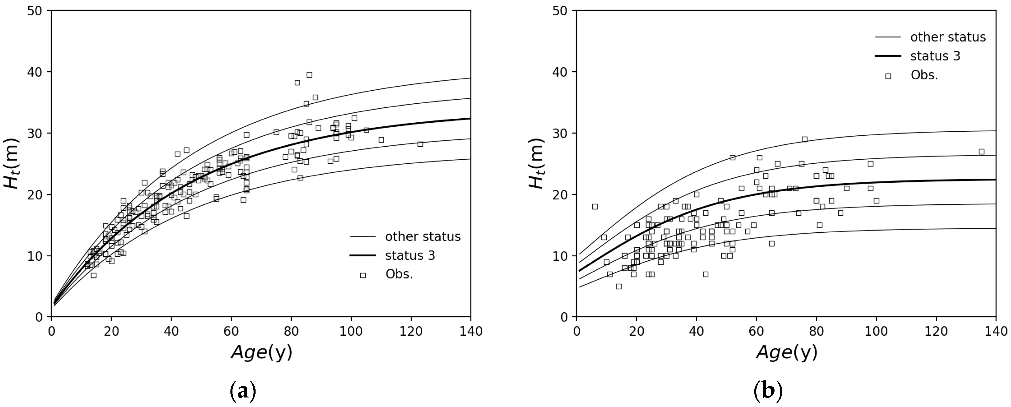
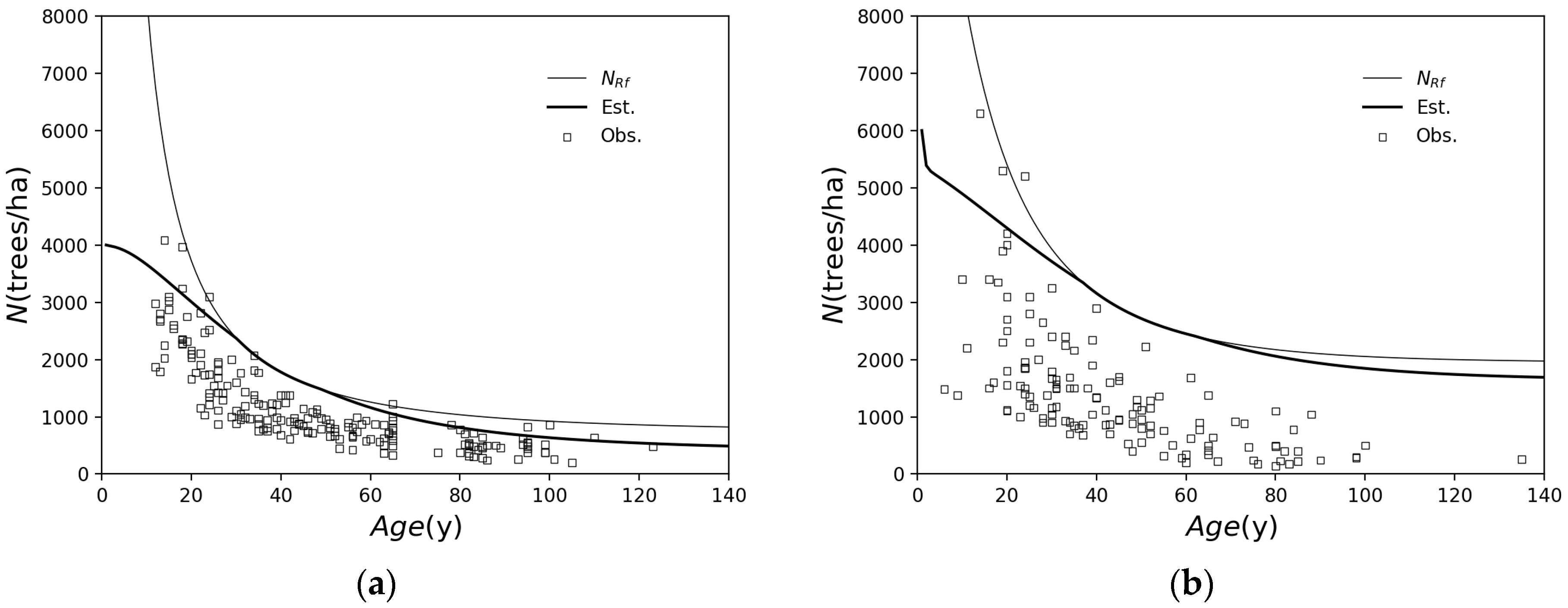
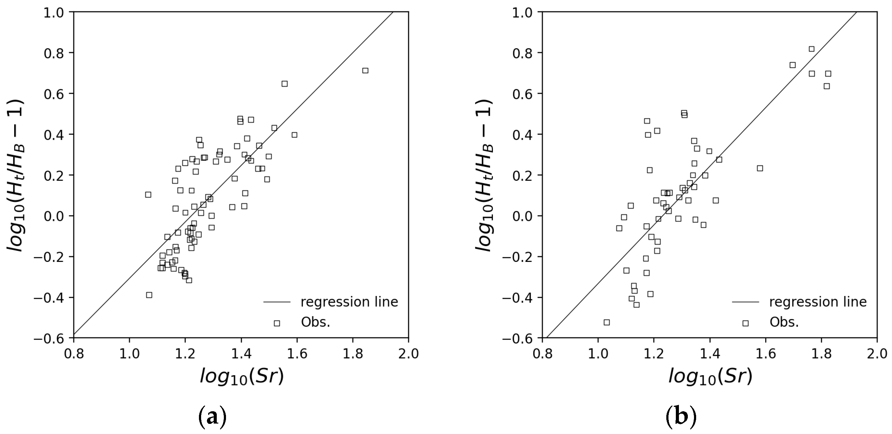
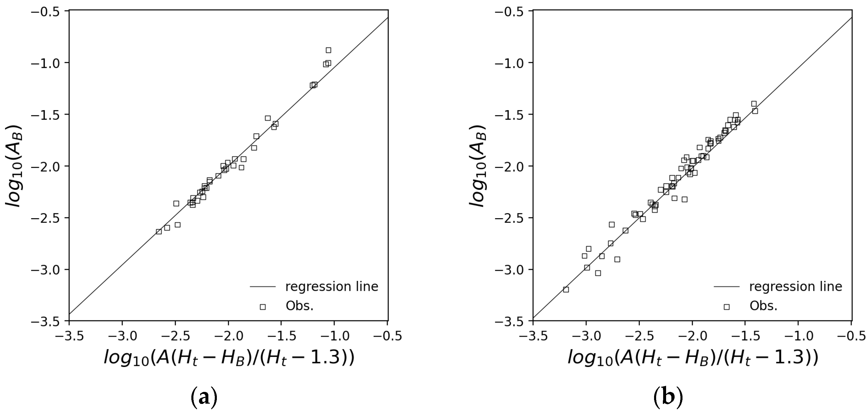
2.1.1. Forest Growth Model

Japanese forestry industries use yield-density diagrams in predicting tree growth and timber harvest [12,13,14,15,16,17,18,19,20]. In this study, the forest growth model was developed based on yield-density diagrams. Tree height of the top layer $H_t$ (m) was defined based on growth curve equations. The growth curves used were the Mitscherlich curve (Equation (1)), logistic curve (Equation (2)), Gompertz curve (Equation (3)), and so on.

$$H_t=M\left\{1-L\exp \left(-Kt\right)\right\}$$

(1)

$$H_t=M/\left(1+L\exp \left(-Kt\right)\right)$$

(2)

$$H_t=\exp \left\{M\left(1-L\exp \left(-Kt\right)\right)\right\}$$

(3)

where $t$ is forest age (y), and $M$, $L,$ and $K$ are parameters determined for each tree species and each area. Variation in growth at the same forest age is adjusted for the growth status. The growth status is a parameter determined for each location based on sunlight, soil, moisture condition, and other factors. In this study, the tree height determined through Equations (1)–(3) was taken as status 3, and the index of statuses 1–5 given to each area was used to represent the variation in growth. The distribution range of statuses was determined so that 95% of the forest sample said to determine the parameters of the growth curves fell between statuses 1 and 5. Figure 1 shows the plots and the growth curves of Japanese cedar (Cryptomeria japonica) and type L-1 broadleaf forests, such as beech (Fagus crenata), Mizunara oak (Quercus crispula), Keyaki (Zelkova serrata), walnut (Juglans), horse chestnut (Aesculus turbinata), and so on, for samples of statuses 1–5.

Stem volume excluding branches and leaves is the so-called “merchantable volume”. The average “merchantable volume” (hereinafter “stem volume”) per hectare $V$ (m³/ha) is obtained from the following inverse formula for the yield-density effect.

$$V={\left(b_1{H_t}^{b_2}+\frac{b_3{H_t}^{b_4}}{N}\right)}^{-1}$$

(4)

where $N$ is the stand density (trees/ha), and $b_1$ to $b_4$ are parameters determined for each tree species and each area. The average diameter at breast height $D$ (cm) is obtained from the following equations:

$$H_F={\alpha }_1+{\alpha }_2{H}_t+\frac{{\alpha }_3\sqrt{N}{H}_t}{100}$$

(5)

$$D_g=200\sqrt{\frac{V}{\pi N{H}_F}}$$

(6)

$$D={\beta }_1+{\beta }_2{D}_g+\frac{{\beta }_3\sqrt{N}{H}_t}{100}$$

(7)

where $H_F$ is the stand shape ratio, $D_g$ is the average section diameter (cm), and ${\alpha }_1$ to ${\alpha }_3$ and ${\beta }_1$ to ${\beta }_3$are parameters determined for each tree species and each area. Stand density varies with forest management, but if the stand is not artificially managed, it decreases due to natural mortality. A smaller stand density for the next year based on the natural mortality curve, defined as per Equation (8), and maximum density $N_{Rf}$ (trees/ha) based on the maximum density curve, defined as per Equation (9), are adopted.

$$\frac{1}{N\left(t+1\right)}=\frac{1}{N_0}-\frac{v\left(t\right)}{K_5{N_0}^{\left(K_1+1\right)}}$$

(8)

$$N_{Rf}=K_4{H_t}^{K_3}$$

(9)

where $N\left(t+1\right)$ is the stand density in year $t+1$, $N_0$ is the planted stand density (trees/ha), and $v\left(t\right)$ is the average stem volume for a stand (m³) in year $t$. $K_1$ to $K_4$ are determined with the parameters $b_1$ to $b_4$ of the inverse formula for the yield-density effect and marginal competition ratio number $R_f$as follows:

$$K_1=\frac{b_4}{b_2-b_4}$$

(10)

$$K_3=b_4-b_2$$

(11)

$$K_4=\frac{b_3\left(1-R_f\right)}{b_1{R}_f}$$

(12)

$$K_5=\frac{K_1{R}_f}{b_3}{\left(\frac{R_f}{1-R_f}\frac{b_1}{b_3}\right)}^{K_1}{\left(\frac{b_2}{b_4}\right)}^{\left(K_1+1\right)}$$

(13)

Figure 2 shows the observed sample forest plots and estimated stand density of Japanese cedar and type L-1 broadleaf forests. The plots with densities less than the natural mortality curves and the maximum density curves indicate locations where densities have decreased due to thinning, etc.

2.1.2. LAI Estimation Model

LAI (leaf area index) is the leaf area per unit area (m²/m²). LAI is obtained with the equation for the relationship of dry leaf weight and leaf area and the equation for the relationship of the breast height diameter and dry leaf weight. Those equations are defined for each tree species. Total leaf weight of a tree is more strongly related to the cross-sectional area under the living branch than the diameter at breast height, including dead conduits, as shown by Shinozaki et al. [21]. Shinozaki’s pipe model is a well-known model in the field of ecology, but very few forest survey data are available, and in many cases, equations have been proposed using the breast height diameter as an alternative to the cross-sectional area under the living branch, for example, in [22,23]. Therefore, in this study, LAI estimation models using the cross-sectional area under the living branch were developed for Japanese cedar and cypress (Chamaecyparis obtusa), for which survey data are abundant, and models using the breast height diameter for other species as follows:

The cross-sectional area under the living branch is related to the height under the branch $H_B$ (m). Although the height under the living branch changes due to forest management practices such as pruning, in a case where there is no artificial care, it is estimated using the following equation proposed by Kanazawa et al. [24]:

$$H_B=\frac{H_t}{{a_0{S}_r}^{a_1}+1}$$

(14)

where $S_r$ is the relative spacing index, defined as follows:

$$S_r=\frac{10000}{H_t\sqrt{N}}$$

(15)

where $a$ and $b$ are parameters determined for each tree species. Equation (14) is modified as follows:

$${\log }_{10}\left(\frac{H_t}{H_B}-1\right)={\log }_{10}{a}_0+a_1{\log }_{10}{S}_r$$

(16)

Figure 3 shows the results of plotting data extracted from several previous studies [22,25,26,27,28,29,30,31,32,33,34,35,36,37,38,39,40]. In this study, the parameters $a_0$ and $a_1$ of Equation (16) are defined as $a_0$ = 0.02039 and $a_1$ = 1.384 for cedar and $a_0$ = 0.01694 and $a_1$ = 1.439 for cypress from Figure 3. The correlations between the observed and the estimated $H_B$, using Equation (16) and the obtained parameters, are $R$ = 0.967 and 0.943 for cedar and cypress, respectively, indicating that the parameters were estimated with good accuracy.

Assuming that the trunk shape is trapezoidal, the following equation is proposed between the cross-sectional area under the living branch $A_B$ (m²) and $H_B$ [27,41]:

$$A_B=A\left(H_t-H_B\right)/\left(H_t-H_0\right)$$

(17)

where $A$ is the cross-sectional area at breast height (m²), and $H_0$ is breast height, which is typically 1.3 m [41]. In this study, the following equation, modified from Equation (17), was used to adjust for small differences among tree species:

$${\log }_{10}{A}_B=c_0{\log }_{10}\left\{A\left(H_t-H_B\right)/\left(H_t-1.3\right)\right\}+c_1$$

(18)

where $c_0$ and $c_1$ are parameters determined for each tree species. Figure 4 shows the results of plotting data extracted from several previous studies [26,29,31,34,36,42,43,44,45]. In this study, the parameters $c_0$ and $c_1$ of Equation (18) are defined as $c_0$ = 0.9558 and $c_1$ = −0.09077 for cedar and $c_0$ = 0.9682 and $c_1$ = −0.08349 for cypress from Figure 4. The correlations between the observed and the estimated $A_B$ are $R$ = 0.980 and 0.983 for cedar and cypress, respectively, indicating that the parameters were estimated with good accuracy.

Many equations have been proposed for estimating dry leaf mass, including one that uses the cross-sectional area and another that uses the square of the diameter. In this study, the following equations, which were relatively accurate for all species analyzed, are proposed:

$${\log }_{10}{W}_L=d_0{\log }_{10}{A}_B+d_1$$

(19)

$${\log }_{10}{W}_L=d_2{\log }_{10}D+d_3$$

(20)

where $W_L$ is the total dry leaf mass of one tree (kg), and $d_0$ to $d_3$ are parameters determined for each tree species. Figure 5 shows the relationships of $W_L$ and $A_B$ with data extracted from several previous studies [22,25,26,27,29,30,31,32,33,34,36,40,41,42,43,44,45,46,47]. In this study, the parameters $d_0$ and $d_1$ of Equation (19) are defined as $d_0$ = 0.9601 and $d_1$ = 2.759 for cedar and $d_0$ = 1.031 and $d_1$ = 2.897 for cypress from Figure 5. The correlations between $A_B$ and $W_L$ are $R$= 0.858 and 0.914 for cedar and cypress, respectively, indicating that the parameters were estimated with good accuracy.

Figure 6 shows the relationships $W_L$ and $D$ with extracted data from several previous studies for beech, Konara oak, and birch [45,48,49,50,51,52,53,54,55].

Table 1. Parameters obtained for Equation (20) and their correlations for beech, Konara oak and birch.

	Beech	Konara Oak	Birch
$d_2$	1.854	1.974	2.278
$d_d$	−1.883	−1.659	−2.290
$R$	0.958	0.858	0.889

shows the obtained parameters and their correlations, as determined from Figure 6. Any correlations are more than 0.85, so good parameters were obtained.

Many equations have been proposed for estimating the leaf area from the dry weight of the leaf. In this study, the following equations, which were relatively accurate for all species analyzed, are proposed:

$$A_L=a{W}_L$$

(21)

where $A_L$ is the total leaf area of one tree (m²), and $a$ is a parameter determined for each tree species. Figure 7 shows the relationships of $A_L$ and $W_L$ with data extracted from several previous studies for cedar, cypress, beech, Konara oak, and birch [26,32,33,36,45,49,51,56,57,58,59,60,61,62,63].

Table 2. Parameters obtained for Equation (21) and their correlations for cedar, cypress, beech, Konara oak and birch.

	Cedar	Cypress	Beech	Konara Oak	Birch
$a$	2.897	3.666	20.77	11.90	17.62
$R$	0.995	0.993	0.998	0.992	0.973

shows the parameters obtained and their correlations, as determined from Figure 7. Any correlations are more than 0.95, so good parameters were obtained.

Finally, LAI is obtained using the stand density as follows:

$$LAI=A_{L}N/10000$$

(22)

where $LAI$ is LAI (m²/m²) and $N$ is stand density (trees/ha). As described in this section, the LAI estimation model is proposed based on forest structural factors such as forest age, tree height, and stand density for several tree species, including broadleaf forest species.

2.2. Hydrological Model

The time variation of the basin storage volume $S$ is expressed using runoff volume $Q$, precipitation $R,$ and evapotranspiration $E$ as follows:

$$\frac{dS}{dt}=R-Q-E$$

(23)

where $t$ is time. Considering the long-term water balance, $dS/dt=0$. Thus, Equation (23) is modified to $Q=R-E$. If the annual water supply is considered as the water conservation function, the estimation of annual evapotranspiration and observation of annual precipitation are important to evaluate the water conservation function for the specific basin. In Japan, rainfall radar observation networks are well developed, so it is possible to estimate annual basin precipitation amounts. Annual evaporation is estimated using the following procedure, which combines the estimation of evapotranspiration and interception evaporation:

Evapotranspiration is obtained using potential evapotranspiration according to the Makkink equation [64], which considers albedo, and correction factors as follows:

$$E_p=\left(a+0.05-\alpha \right)\frac{\mathsf{\Delta }}{\mathsf{\Delta }+\gamma }\frac{R_s}{\iota }+b$$

(24)

where $E_p$ is daily potential evapotranspiration (mm/d), $\gamma$ is the psychrometric coefficient, $\mathsf{\Delta }$ is the gradient of the saturated vapor pressure curve (hPa/°C), $R_s$ is the total solar radiation (MJm⁻²d⁻¹), $\iota$ is latent heat of evaporation (MJ/kg), $\alpha$ is albedo, and $a$ and $b$ are parameters for each location. The difference between actual and possible evapotranspiration varies depending on the condition of the ground surface, vegetation, and so on. Kondo [65] proposed the following correction factors using LAI:

$$\frac{E_t}{E_p}=\frac{0.78}{1+\exp \left\{-0.78\left(LAI-2.2\right)\right\}}$$

(25)

$$\frac{E_t}{E_p}=0.45+0.4\left\{1-\exp \left(-1.5LAI\right)\right\}$$

(26)

where $LAI$ is LAI (m²/m²), and $E_t$ is daily actual evapotranspiration (mm/d). Equations (25) and (26) are used for forest area and grassland, respectively.

Interception evaporation is estimated according to the following method proposed by Kondo et al. [66,67,68]:

$$I=I_{POT}\times \left(\tau /24\right)+S$$

(27)

where $I$ is interception evaporation (mm), $I_{POT}$ is the potential interception evaporation (mm), $\tau$ is the duration of a rainfall event (h), and $S$ is the water storage capacity of tree surfaces (mm). $I_{POT}$ is defined using the following equation:

$$\frac{{\iota I}_{POT}}{R_n-G-\sigma T^4}=\frac{\mathsf{\Delta }}{\gamma }\left\{T^{+}+q^{+}\left(1-rh\right)\right\}J$$

(28)

where $R_n$ is the net radiation (W/m²), $G$ is the ground heat flux (W/m²), $T$ is the air temperature (K), $rh$ is relative humidity, and $\sigma$ is the Stefan–Boltzmann constant. $T^{+}$, $q^{+}$, and $J$ are defined using the following equations:

$$T^{+}=\frac{1-J\left(\mathsf{\Delta }/\gamma \right)\left(1-rh\right)q^{+}}{1+J\left(1+\mathsf{\Delta }/\gamma \right)}$$

(29)

$$q^{+}=\frac{1}{R_n-G-\sigma T^4}\frac{4\sigma T^3{q}_{sat}\left(T\right)}{\mathsf{\Delta }}$$

(30)

$$J=\left(c_P\rho /4\sigma T^3\right)C_{H}u$$

(31)

where $q_{sat}\left(T\right)$ is the saturated specific humidity at air temperature $T$, $u$ is wind speed, $c_P$ is the constant pressure specific heat of air (1006 J/kg/K at 1.0 a.t.m.), $\rho$ is the wet gas density (kg/m³), and $C_H$ is the bulk exchange coefficient for sensible heat. The water storage capacity $S$ is defined using the following equation:

$$S=s_{leaf}LAI+s_{branch}BAI+s_{stem}SAI$$

(32)

where $BAI$ is the branch area index (BAI), which is the branch area per unit area (m²/m²), and $SAI$ is the stem area index (SAI), which is the stem area per unit area (m²/m²). $s_{leaf}$, $s_{branch}$, and $s_{stem}$ are the water storage capacity of the leaf, branch, and stem (mm/$LAI$, mm/$BAI$, mm/$SAI$), respectively. $BAI$ was estimated using the cedar and cypress tree shape model proposed by Ebisu et al. [69]. For other species, the mean of the parameters for cedar and cypress was used instead. $SAI$ considers the tree shape as a triangular pyramid and calculates the surface area of the triangular pyramid with the cross-sectional area at breast height as the base area and the height of the tree as the height of the triangular pyramid.

Here, the probability of precipitation impacting a tree body $\Omega *$ is defined using the following equation:

$$\Omega *=\Omega \left\{1-\mathrm{e}\mathrm{x}\mathrm{p}\left(-\frac{f·LAI}{\Omega }\right)\right\}$$

(33)

where $\Omega$ is the canopy closure rate, and $f$ is the factor of leaf tilt, usually 0.5. In the case of $\Omega *\times P_g>I_{POT}\times \left(\tau /24\right)+S$, canopy interception can be estimated as $I=I_{POT}\times \left(\tau /24\right)+S$; otherwise, $I=\Omega *\times P_g$, where $P_g$ is gross precipitation (mm). $\Omega$ is expressed based on the Beer–Lambert law as follows:

$$1-\Omega =\mathrm{e}\mathrm{x}\mathrm{p}\left(-k·LAI\right)$$

(34)

where $k$ is the extinction coefficient, affected by the angle of the leaves. In this study, the relationship of $1-\Omega$ and LAI was plotted in Figure 8 [70,71], and the value of $k$ = 0.4035 ($R$ = 0.892) was obtained.

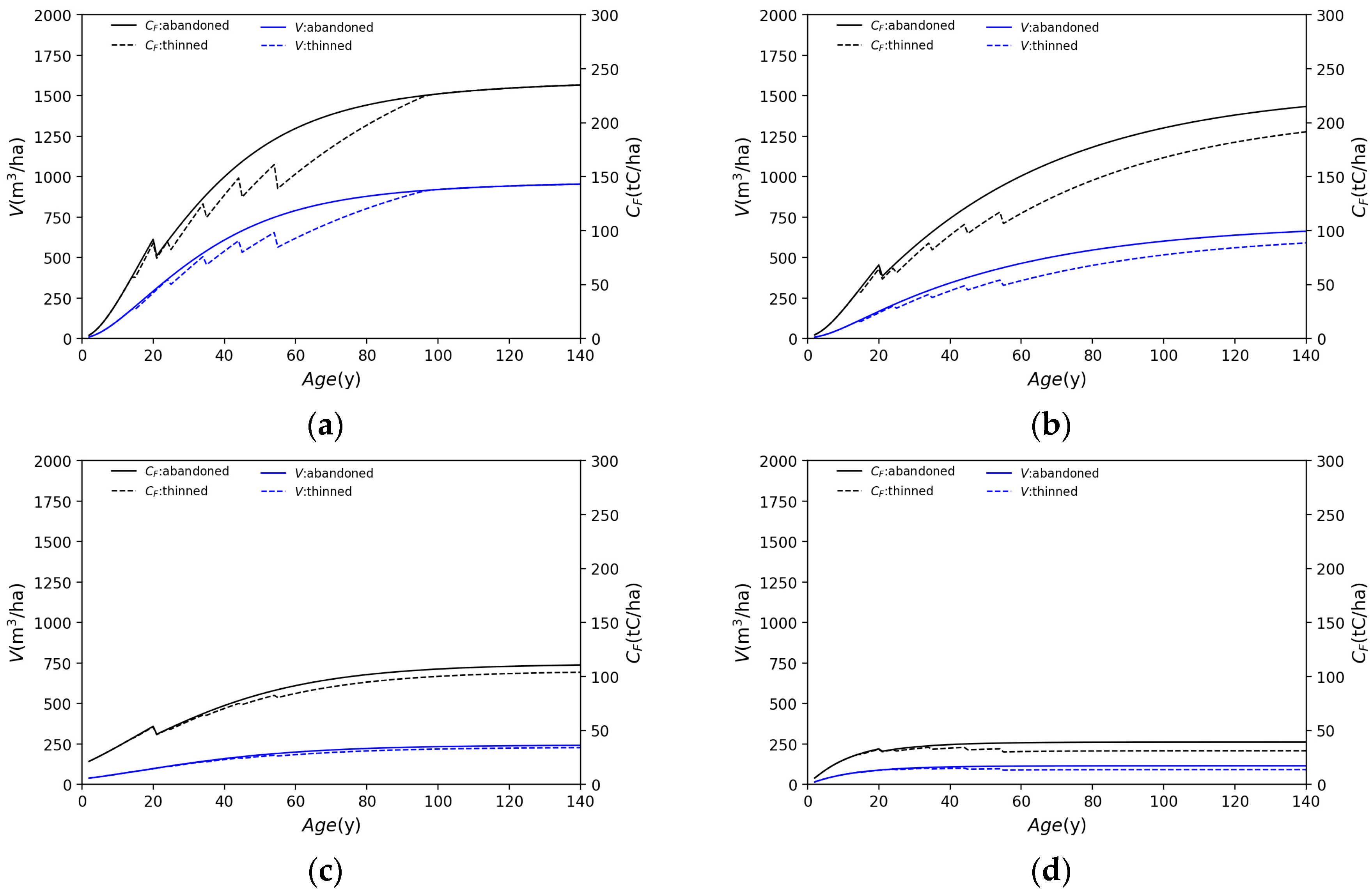
2.3. Carbon Stock Assessment Model

In this study, the carbon stock in living biomass in forest $C_F$ (t-C/ha) was calculated using the following equation, based on a greenhouse gas inventory report by the CGER, Japan [72]:

$$C_F=V·D_d·BEF·\left(1+R_{root}\right)·CF$$

(35)

where $V$is the stem volume per hectare (m³/ha), $D_d$is the dry wood density (t/m³), $BEF$ is the biomass expansion factor for the conversion of merchantable volume, $R_{root}$ is the root-to-shoot ratio, and $CF$ is the carbon fraction of dry matter (t-C/t). Thus, $V·BEF·\left(1+R_{root}\right)$ reflects the total volume of trees, including leaves, branches, roots, and stem. Parameters for the major tree species are listed in

Table 3. Parameters for estimations of living biomass for each species [66].

		Cedar	Cypress	Beech	Oak	Birch
$BEF$	$\le 20$	1.57	1.55	1.58	1.40	1.31
	$>20$	1.23	1.24	1.32	1.26	1.20
$R_{root}$		0.25	0.26	0.26	0.26	0.26
$D_d$		0.314	0.407	0.573	0.624	0.438
$CF$		0.51	0.51	0.48	0.48	0.48

Note—$BEF$: biomass expansion factor (20 = age); $R_{root}$: root-to-shoot ratio; $D_d$: dry wood density; $CF$: carbon fraction; Cedar: Cryptomeria japonica; Cypress: Chamaecyparis obtusa; Beech: Fagus crenata; Oak: Quercus; Birch: Betula.

.

3. Results and Discussion

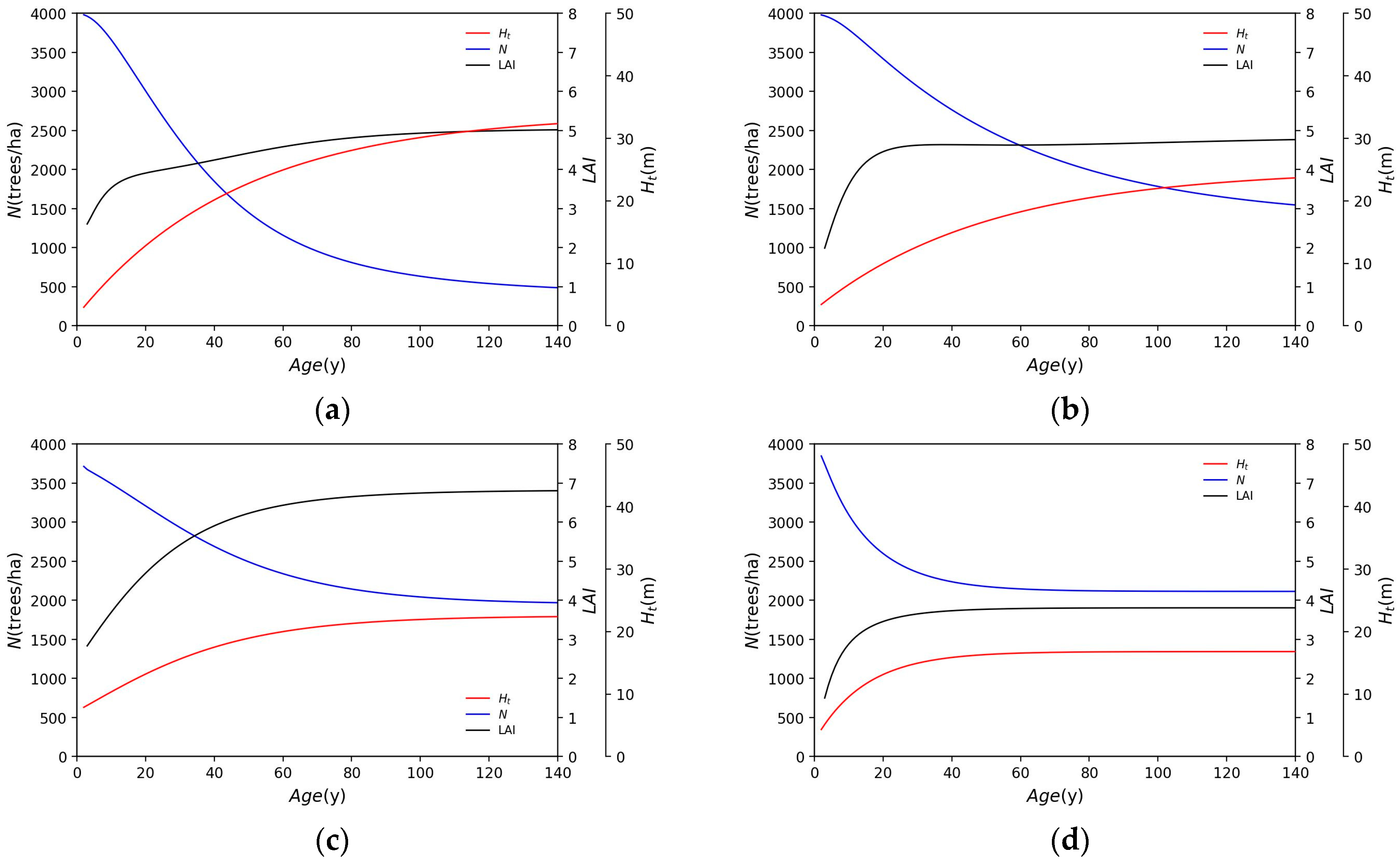
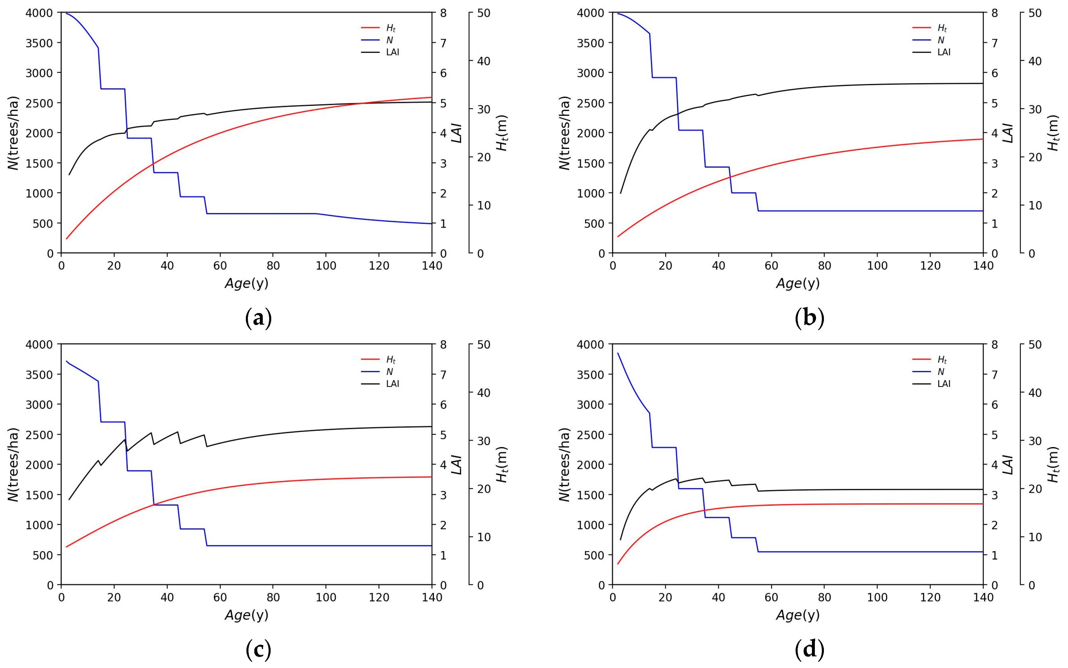
3.1. Application of Each Species

From the above, a model that evaluates water conservation function, carbon stock, and woody production by calculating forest parameters based on tree species, forest age, stand density, and growth status was developed. Figure 9 shows the simulated changes in LAI, stand density, and tree height with forest age in a case where the initial number of trees planted is 4000 trees/ha and the growth status is 3, using the proposed model in this study. The target area is assumed to be Gujo City, Gifu Prefecture, Japan. The density of cedar trees decreases rapidly due to natural mortality, while the density of other tree species decreases relatively slowly. The LAI of beech has a maximum of about 7, while the LAI of Japanese cedar and Japanese cypress has a maximum of about 5. On the other hand, the LAI of birch is up to 4. This shows that the LAI varies depending on the species, or even among the same broadleaf trees.

Figure 10 shows the simulated changes in LAI, stand density, and tree height with forest management as 30% thinning at 25, 35, 45, and 55 years, respectively, versus Figure 9. Cedar is less affected by thinning, except for a small increase in LAI when thinned. Thinning of cypress increases LAI. This is the reason why a decrease in the living branch height and an increase in the living branch cross-sectional area are caused by a decrease in tree density. The LAIs of beech and birch decrease with thinning. Although not the same for all forest management and forest conditions, thinning like that for the management of cedar and cypress is excessive for beech and birch. Excessive thinning greatly reduces the number of trees, resulting in a large decrease in LAI. The example analysis presented in this section assumes growth status 3 and the initial planting of 4000 trees/ha and does not simulate a real forest. Nonetheless, the development of this model enables us to evaluate the impact of forest management on a forest with diverse tree species.

Figure 11 shows the simulated changes in the water supply evaluation factors, such as annual water supply, annual evapotranspiration, and annual interception evaporation. The target area is assumed to be Gujo City, Gifu Prefecture, Japan. The water supply for each species is simulated using observation data from the Hachiman gauge station, Japan Meteorological Agency. Meteorological data from 1994, the most severe drought year in the past 30 years, are used. Water supply varies with tree species, but generally decreases until about 40 years old, after which it is near constant. Although beech forests have a larger LAI than needleleaf forests, water supply is not significantly different. The reasons for this are not only differences in LAI but also differences in the water storage capacity per unit area and differences in albedo between the broadleaf forest and needleleaf forest. The modified Makkink equation allows us to estimate that the possible evapotranspiration of the broadleaf forest is less than that of the needleleaf forest due to differences in albedo. When applying this calculation, the albedos of the broadleaf and needleleaf forest are $\alpha$ = 0.20 and 0.15, respectively. Water supply does not change much in cedar, decreases in cypress, and increases in beech and birch as a result of LAI changes due to thinning. Yamamura et al. [5] also reported in their model analysis that the water conservation function decreases with forest growth up to a certain forest age and then tends to be almost constant. Vertessy et al. [73] also reported that the water balance and discharge in the watershed of mountain ash forests after forest burns decreased with forest growth up to a certain age, and it becomes almost constant thereafter. Kojima [74] analyzed daily water discharge over about 20 years in a small forested watershed with a cypress priority, and reported a slight decline trend in discharge in a well-grown forest. Our proposed model reproduced the trend reported in the above studies that “the water conservation function declines up to a certain forest age and then becomes almost constat”, which can evaluate water conservation function with high accuracy.

Figure 12 shows the simulated changes in the stem volume and carbon stock per unit area. Figure 12 shows that needleleaf forests accumulate a very large amount of carbon stock, while broadleaf forests accumulate less carbon. For other species besides cedar, the accumulated carbon stock is reduced via thinning. When considering forests as carbon sinks, planting cedar trees was found to be the most effective using this model.

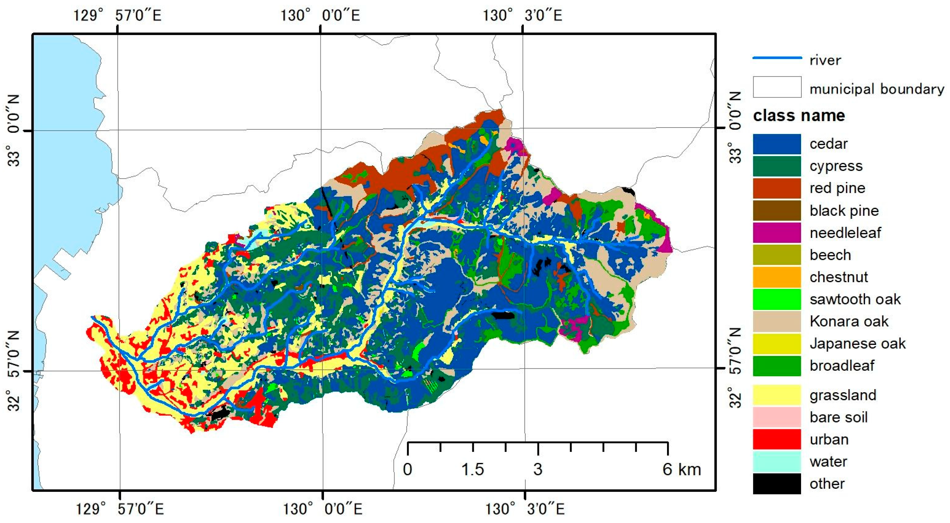
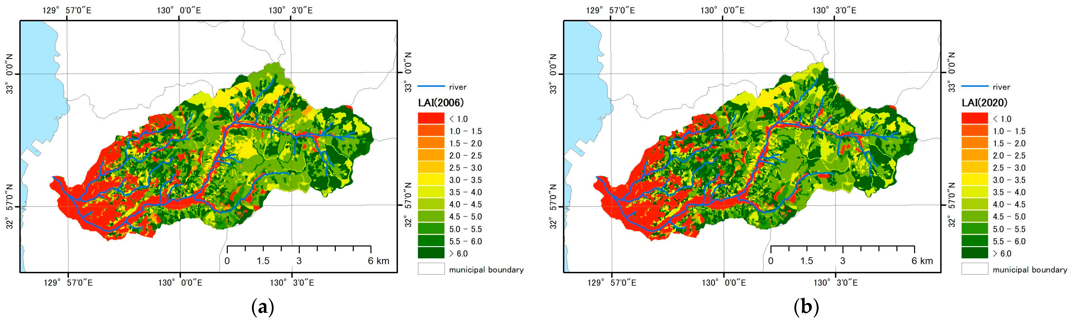
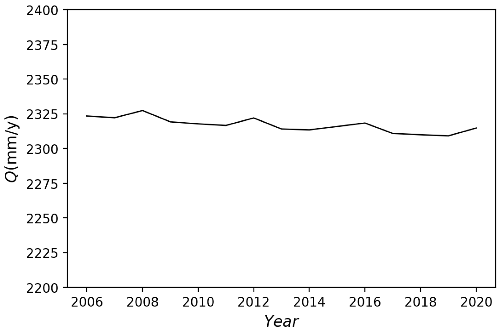
3.2. Basin-Scale Application

3.2.1. LAI Estimation

The model is applied to the Kori River Basin in Omura City, Nagasaki Prefecture. This basin (54.7 km²) has a relatively mild climate with an average annual temperature of about 17 °C and annual rainfall of about 1800 mm, with the Kayase Dam (total storage capacity: 6.8 Mm³) in its upper reaches. Figure 13 shows the distribution of tree species and land cover types in the target basin. The basic forest information, such as species, age, and growth status, was obtained from the Omura City Forest Inventory for FY2020, the National Forest Inventory for FY2021, and Natural Environmental GIS by the Biodiversity Center of Japan [75]. The forest conditions from 2006 to 2020 were estimated using the forest model described above, based on the forest management history, such as thinning, clear-cutting, and harvest rate. Figure 14 shows the distribution of LAI in 2006 and 2020, estimated with the forest model. The LAI increases in some areas between 2006 and 2020 due to growth, while the LAI decreases in other areas due to forest management such as logging, clear-cutting, and thinning.

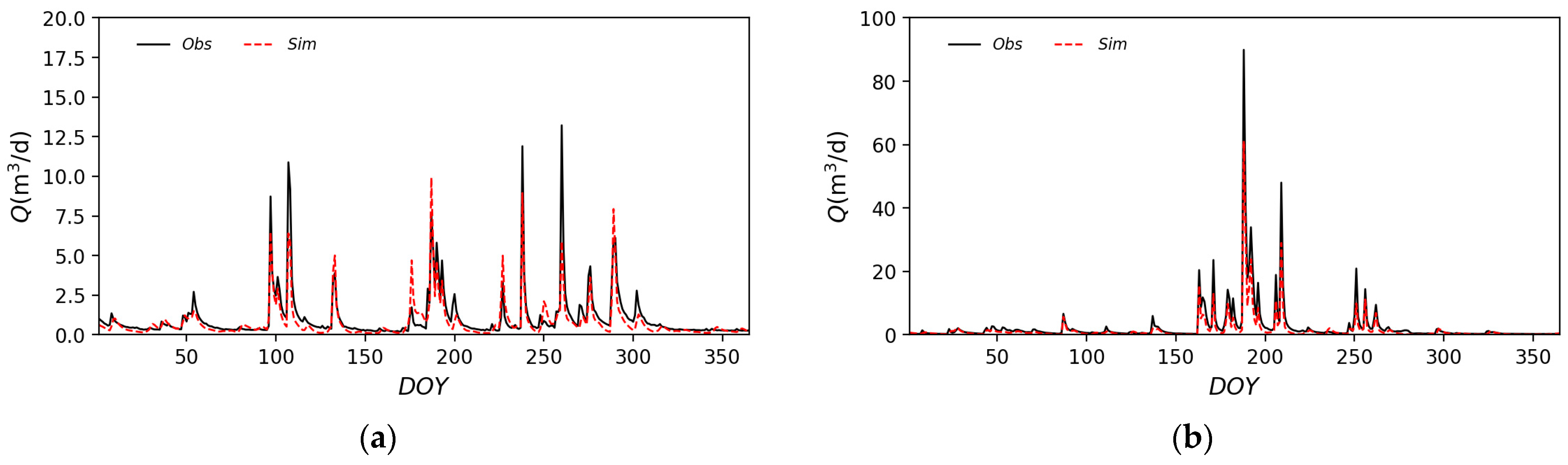
3.2.2. Hydrological Application and Validation

Using the hydrological model described above, daily effective rainfall was calculated by subtracting daily interception evaporation and evapotranspiration from total precipitation, and daily discharge at the Kayaba Dam was calculated using a simple runoff model. Figure 15 compares the observed and simulated inflow hydrographs at the Kayaba Dam in 2017 with a drought trend and in 2020 with a heavy rainfall event. Peak flow rates were slightly underestimated, but generally good results were obtained.

Table 4. Accuracy of simulation results for each year.

	2016	2017	2018	2019	2020
NSE	0.875	0.774	0.823	0.848	0.848

shows validation results based on the Nash–Sutcliffe efficiency (NSE). An NSE of more than 0.7 was obtained for all years, indicating that the flow rate could be calculated with good estimation accuracy. The annual water supply in the Kori River Basin was evaluated based on the LAI distribution for 2006 to 2020. Meteorological conditions were unified for the year 2020. Figure 16 shows the variation in annual water supply. We found that changes in LAI associated with forest management can result in slight variations in water supply with the same meteorological data. However, the change is very small, at less than 1% of the total, suggesting that the forest management practices currently in place do not have a significant impact on water supply.

4. Conclusions

In this study, we developed an integrated tool to evaluate how ecosystem services such as the water conservation function, wood production, and carbon absorption are changed by forest management practices such as clear-cutting, thinning, pruning, and tree species shifting for sustainable forest management. Previous studies have classified conifers and broadleaf trees, and evergreen and deciduous trees, but have been insufficient to cover the diversity of tree species in Japan. In Japan, there are many observations and developed models for cedar and cypress for timber production purposes, but models to evaluate species differences have been lacking for other trees, especially for broadleaf trees. By referring to many previous reports and combining data, we developed a model for multiple tree species, which can evaluate changes that may occur as a result of species conversion and forest management in each species.

The results of our simulations for the major tree species produced the following findings:

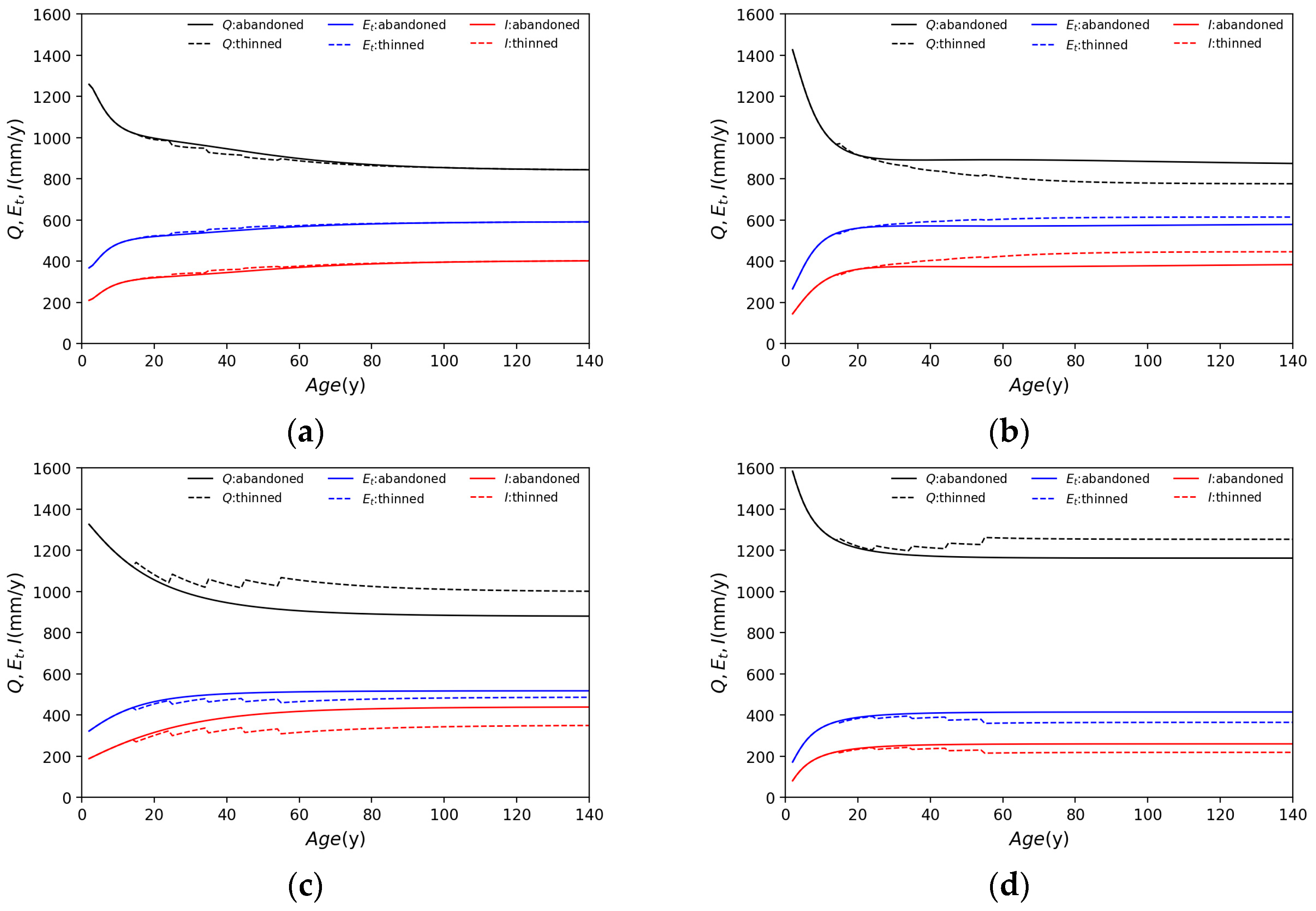
• Water supply varies with tree species but generally decreases until about 40 years of age, after which it is near constant.
• Cedar is less affected than other tree species by thinning. The water supply is barely affected by thinning.
• The thinning of cypress trees increases the LAI due to reduced density, and water supply is reduced in thinned forests compared to in abandoned forests, influenced by an increased LAI.
• Although beech forests have a larger LAI than needleleaf forests, water supply is not significantly different.
• Birch has a smaller LAI and a much larger water supply than other species.
• Broadleaf forests are more affected by thinning than needleleaf forests and tend to receive an increased water supply as a result of thinning.

Our model also enables the evaluation of the water conservation function at the basin scale. Application to the Kori River Basin, Omura City, Nagasaki Prefecture, Japan, showed that large-scale clear-cutting and species conversion may have an impact, but the forest management currently practiced by Omura City does not result in significant changes in forest function.

To summarize, in this study, we developed a model to evaluate forest modification and changes in function for diverse tree species. In the future, we would like to use this model to examine the degree to which forest conditions change and whether that is to the extent that significant alterations in forest function occur, as well as the relationship between the costs of forest management and the ecosystem services that change.

References

1. Bagstad, K.J.; Johnson, G.W.; Voigt, B.; Villa, F. Spatial dynamics of ecosystem service flows: A comprehensive approach to quantifying actual services. Ecosyst. Serv. 2013, 4, 117–125. [Google Scholar] [CrossRef]
2. Government Public Relations Office, Japan. Public Opinion Survey on Forest and Livelihoods. Available online: https://survey.gov-online.go.jp/r01/r01-sinrin/ (accessed on 5 December 2023). (In Japanese)
3. Kohsaka, R.; Uchiyama, Y. Status and Trends in Forest Environment Transfer Tax and Information Interface between Prefectures and Municipalities: Multi-Level Governance of Forest Management in 47 Japanese Prefectures. Sustainability 2022, 14, 1791. [Google Scholar] [CrossRef]
4. Thornton, P.E.; Law, B.E.; Gholz, H.L.; Clark, K.L.; Falge, E.; Ellsworth, D.S.; Goldstein, A.H.; Monson, R.K.; Hollinger, D.; Falk, M.; et al. Modeling and measuring the effects of disturbance history and climate on carbon and water budgets in evergreen needleleaf forests. Agric. For. Meteorol. 2002, 113, 185–222. [Google Scholar] [CrossRef]
5. Yamaura, Y.; Yamada, Y.; Matsuura, T.; Tamai, K.; Taki, H.; Sato, T.; Hashimoto, S.; Murakami, W.; Toda, K.; Saito, H.; et al. Modeling impacts of broad-scale plantation forestry on ecosystem services in the past 60 years and for the future. Ecosyst. Serv. 2021, 49, 101271. [Google Scholar] [CrossRef]
6. Cheng, X.; Bai, Y.; Zhu, J.; Han, H. Effects of forest thinning on interception and surface runoff in Larix principis-rupprechtii plantation during the growing season. J. Arid Environ. 2020, 181, 104222. [Google Scholar] [CrossRef]
7. Chen, L.; Yuan, Z.; Shao, H.; Wang, D.; Mu, X. Effects of Thinning Intensities on Soil Infiltration and Water Storage Capacity in Chinese Pine-Oak Mixed Forest. Sci. World J. 2014, 2014, 268157. [Google Scholar] [CrossRef]
8. Komatsu, H. Relationship between Stem Density and Interception Ratio for Coniferous Plantation Forests in Japan. J. Jpn. For. Soc. 2007, 89, 217–220. (In Japanese) [Google Scholar] [CrossRef]
9. Watanabe, N.; Kojima, T.; Shinoda, S.; Ohashi, K.; Tamagawa, I.; Saitoh, T. Observation and Modeling of Rainfall Interception in Evergreen Forest and Deciduous Forest. J. Jpn. Soc. Civ. Eng. Ser. B1 Hydraul. Eng. 2012, 68, I_1759–I_1764. (In Japanese) [Google Scholar] [CrossRef]
10. Komatsu, H.; Shinohara, Y.; Kume, T.; Otsuki, K. Changes in peak flow with decreased forestry practices: Analysis using watershed runoff data. J. Environ. Manag. 2011, 92, 1528–1536. [Google Scholar] [CrossRef]
11. Gao, X.; Huang, X.; Chang, S.; Dang, Q.; Wen, R.; Lo, K.; Li, J.; Yan, A. Long-term improvement in water conservation function at Qilian Mountain national Park northwest China. J. Mt. Sci. 2023, 20, 2885–2897. [Google Scholar] [CrossRef]
12. Forestry Resources Management Division of Gifu Prefecture. Forest Harvest Table/Forest Density Control Chart for Japanese Cedar Planted Forest; Forestry Resources Management Division of Gifu Prefecture: Gifu, Japan, 1992. (In Japanese)
13. Forestry Resources Management Division of Gifu Prefecture. Forest Harvest Table/Forest Density Control Chart for Japanese Cypress Planted Forest; Forestry Resources Management Division of Gifu Prefecture: Gifu, Japan, 1992. (In Japanese)
14. Forestry Resources Management Division of Gifu Prefecture. Forest Harvest Table/Forest Density Control Chart for Japanese Redpine Planted Forest; Forestry Resources Management Division of Gifu Prefecture: Gifu, Japan, 1984. (In Japanese)
15. Forestry Resources Management Division of Gifu Prefecture. Forest Harvest Table/Forest Density Control Chart for Japanese Larch Planted Forest; Forestry Resources Management Division of Gifu Prefecture: Gifu, Japan, 1985. (In Japanese)
16. Forestry Resources Management Division of Gifu Prefecture. Forest Harvest Table/Forest Density Control Chart for Broad Leaf Forest; Forestry Resources Management Division of Gifu Prefecture: Gifu, Japan, 1992. (In Japanese)
17. Maeda, H. Management standard for Hinoki (Chamaecyparis obtuse) plantations applied to long-term management in Nagasaki prefectures. Bull. Nagasaki Agric. For. Technol. Dev. Cent. 2012, 3, 54–64. (In Japanese) [Google Scholar]
18. Forestry Experiment Station, Kyushu Region Hinoki Forest Harvest Table Adjustment Instructions. Harvest Table Adjustment Operations Research Materials, 19; Kumamoto For. Off., Forest Agency: Kumamoto, Japan, 1957; p. 49. (In Japanese)
19. Forestry Experiment Station, Kitakyushu Region Akamatsu Forest Harvest Table Adjustment Instructions. Harvest Table Adjustment Operations Research Materials, 25; Kumamoto For. Off., Forest Agency: Kumamoto, Japan, 1960; p. 46. (In Japanese)
20. Narasaki, K.; Maeda, H.; Sasaki, S. Adjustment of Japanese cedar forest density control chart and status index curve for preparation of Fukuoka Prefecture version of system harvest table. Bull. Fukuoka Agric. For. Res. Cent. 2015, 1, 38–43. (In Japanese) [Google Scholar]
21. Shinozaki, K.; Yoda, K.; Hozumi, K.; Kira, T. A Quantitative Analysis of Plant Form-The Pipe Model Theory I. Basic Analyses. Ecol. Soc. Jpn. 1964, 14, 97–105. [Google Scholar]
22. Ando, T.; Hatiya, K.; Doi, K.; Kataoka, H.; Kato, Y.; Sakaguchi, K. Studies on the system of density control of sugi (Cryptomeria japonica) stand. Bull. Gov. For. Exp. Stn. 1968, 209, 1–76. (In Japanese) [Google Scholar]
23. Makungwa, S.D.; Kodani, J. Estimation of standing crop and productivity of an even-aged young Keyaki (Zelkova serrata Makino) plantation in Suzu prefectural Forest. Bull. Ishikawa-Ken For. Exp. Stn. 1998, 29, 6–11. (In Japanese) [Google Scholar]
24. Kanazawa, Y.; Kiyono, Y.; Fujimori, T. Crown Development and Stem Growth in Relation to Stand Density in Even-Aged Pure Stands (II) Cear-Length Model of Cryptomeria japonica Stands as a Function of Stand Density and Tree Height. J. Jpn. For. Soc. 1985, 67, 391–397. [Google Scholar]
25. Watanabe, H.; Moteki, Y. Growth progress and biomass in 92-years-old plantation of Japanese cedar. Bull. Gifu Prefect. Res. Inst. For. 2007, 36, 7–13. (In Japanese) [Google Scholar]
26. Ishii, T.; Nashimoto, M.; Shimogaki, H. Development of forest observation method using remote sensing data -Estimation of leaf area index-. In Annual Research Report; Central Research Institute of Electric Power Industry: Tokyo, Japan, 1998. (In Japanese) [Google Scholar]
27. Inagaki, Y.; Nakanishi, A.; Tange, T. A simple method for leaf and branch biomass estimation in Japanese cedar plantations. Trees 2020, 34, 349–356. [Google Scholar] [CrossRef]
28. Saito, H.; Kan, M.; Shidei, T. Studies on the effects of thinning from small diameter trees (I). Changes in stand condition before and after thinning. Bull. Kyoto Univ. For. 1966, 38, 50–67. (In Japanese) [Google Scholar]
29. Saito, H.; Yamada, I.; Shidei, T. Studies on the effects of thinning from small diameter trees (II). Changes in stand condition after single growing season. Bull. Kyoto Univ. For. 1967, 39, 64–78. (In Japanese) [Google Scholar]
30. Saito, H.; Tamai, S.; Ogino, K.; Shidei, T. Studies on the effects of thinning from small diametered trees (III). Changes in stand condition after the second growing season. Bull. Kyoto Univ. For. 1968, 40, 81–92. (In Japanese) [Google Scholar]
31. Saito, H.; Shidei, T. Studies on the productivity and its estimation methodology in a young stand of Cryptomeria japonica D. Don. J. Jpn. For. Soc. 1973, 55, 52–62. (In Japanese) [Google Scholar]
32. Tadaki, Y.; Kawasaki, Y. Studies on the production structure of forest. IX. Primary productivity of a young Cryptomeria plantation with excessively high stand density. J. Jpn. For. Soc. 1966, 48, 55–61. [Google Scholar]
33. Tadaki, Y.; Ogata, N.; Nagatomo, Y. Studies on production structure of forest. XI. Primary productivities of 28-years-old plantations of Cryptomeria of cuttings and of seedlings origin. Bull. Gov. For. Exp. Stn. 1967, 199, 47–65. (In Japanese) [Google Scholar]
34. Inagaki, Y.; Miyamoto, K.; Itou, T.; Kitahara, F.; Sakai, H.; Okuda, S.; Noguchi, M.; Mitsuda, Y. Estimation of leaf biomass cypress plantation in Kochi Prefecture. Appl. For. Sci. 2015, 24, 11–18. (In Japanese) [Google Scholar]
35. Inagaki, Y.; Fukata, H.; Noguchi, K.; Kuramoto, S.; Nakanishi, A. Recovery of leaf biomass after thinning of hinoki cypress plantations in Kochi Prefecture. Appl. For. Sci. 2018, 27, 1–9. (In Japanese) [Google Scholar]
36. Ishii, T. Estimation of Forest Leaf Area Index Using Remote Sensing Data and Its Applications to Predicting Forest Carbon Sequestration and Water Budget. Ph.D. Thesis, Waseda University, Tokyo, Japan, 2007. (In Japanese). [Google Scholar]
37. Wakiyama, Y.; Onda, Y.; Nanko, K.; Mizugaki, S.; Kim, Y.; Kitahara, H.; Ono, H. Estimation of temporal variation in splash detachment in two Japanese cypress plantations of contrasting age. Earth Surf. Process. Landf. 2010, 35, 995–1005. [Google Scholar] [CrossRef]
38. Nakaya, K.; Wakamatsu, T.; Ikeda, H.; Abe, S.; Toyoda, Y. Development of raindrop kinetic energy model under canopy for the estimation of soil erosion in forest. In Annual Research Report; Central Research Institute of Electric Power Industry: Tokyo, Japan, 2011. (In Japanese) [Google Scholar]
39. Takeuchi, I.; Kawasaki, T.; Mori, S. Changes of stem height-to-diameter ratio in hinoki (Chamaecyparis obtuse) young man-made stands. J. Jpn. For. Soc. 1997, 79, 137–142. (In Japanese) [Google Scholar]
40. Watanabe, H.; Moteki, Y.; Obora, T. Effects of Thinning on Stand Structure and Diameter Growth in Old and Overcrowded Japanese Cypress (Chamaecyparis obtuse) Stands. J. Jpn. For. Soc. 2015, 97, 182–185. (In Japanese) [Google Scholar] [CrossRef]
41. Sumida, A.; Nakai, T.; Yamada, M.; Ono, K.; Uemura, S.; Hara, T. Ground-Based Estimation of Leaf Area Index and Vertical Distribution of Leaf Area Density in a Betula ermanii Forest. Silva Fenn. 2009, 43, 799–816. [Google Scholar] [CrossRef]
42. Kawanabe, S.; Ando, M. Studies on regeneration of natural forest on lower limit of cool temperate deciduous broad-leaved forest V -Biomass and growth in natural forest of Cryptomeria japonica-. Bull. Kyoto Univ. For. 1988, 60, 67–76. (In Japanese) [Google Scholar]
43. Tange, T.; Murakawa, I. Growth and Biomass of an 87-year-old Manmade Chamaecyparis obtuse Stand. Bull. Univ. Tokyo For. 1990, 82, 103–112. (In Japanese) [Google Scholar]
44. Utsugi, H. Effects of Leaf Community Structure on Forest Canopy Photosynthetic Production in a Forest Community: Particularly on the Effect of Leaf Tilt Angle. Ph.D. Thesis, The University of Tokyo, Tokyo, Japan, 2009. (In Japanese). [Google Scholar]
45. Daniel, S.F.; Remko, A.D.; Masae, I.I.; Diego, R.B.; Richard, G.F.; Angelica, V.; Masahiro, A.; Makoto, A.; Niels, A.; Michael, J.A.; et al. BAAD: A Biomass and Allometry Data Base for woody plants. Ecology 2015, 96, 1445. [Google Scholar] [CrossRef]
46. Tange, T.; Kojima, K. Aboveground biomass data of Anno growth monitoring stands of Cryptomeria japonica in the University Forest in Chiba, The University of Tokyo. Misc. Inf. Univ. Tokyo For. 2010, 49, 1–6. (In Japanese) [Google Scholar]
47. Sugimoto, T.; Ishii, H.; Chiba, Y.; Kanazawa, Y. Branch and Foliage Mass and their Vertical Distribution in a 90-year-old Chamaecyparis obtuse Plantation. J. Jpn. For. Soc. 2010, 92, 63–71. (In Japanese) [Google Scholar] [CrossRef]
48. Karizumi, N. (Ed.) The Latest Illustrations of Tree Roots; Seibundo Shinkosha Publishing Co., Ltd.: Tokyo, Japan, 2010; ISBN 978-4-416-41005-9. (In Japanese) [Google Scholar]
49. Tadaki, Y.; Hatiya, K.; Tochiaki, K. Studies on the Production Structure of Forest (XV) Primary Productivity of Fagus crenata in Plantation. J. Jpn. For. Soc. 1969, 51, 331–339. (In Japanese) [Google Scholar]
50. Kotani, J. Estimation of standing crop and productivity of an even-aged young Buna (Fagus crenata) plantation. Bull. Ishikawa-Ken For. Exp. Stn. 2008, 40, 12–16. (In Japanese) [Google Scholar]
51. Hoshi, H.; Tatsuhara, S.; Abe, N. Estimation of Leaf Area Index in Natural Deciduous Broad-leaved Forests Using Landsat TM Data. J. Jpn. For. Soc. 2001, 83, 315–321. (In Japanese) [Google Scholar]
52. Kai, S. Dry-matter production of a young Konara oak (Quercus serrata Thunb.) plantation. Kyushu J. For. Res. 2011, 64, 130–131. (In Japanese) [Google Scholar]
53. Katakura, M.; Koyama, Y. Existing and carbon stocks in larch, red pine, and Konara oak forests, and changes in soil carbon content after logging of red pine forests. Bull. Nagano Prefect. For. Res. Cent. 2007, 22, 33–55. (In Japanese) [Google Scholar]
54. Ogasawara, R.; Yamamoto, T.; Arita, T. Biomass and Production of the Konara (Quercus serrata) Secondary Stand. Hardwood Res. 1987, 4, 257–262. (In Japanese) [Google Scholar]
55. Hasegawa, M. Productivity of Oak Coppice Forests. J. Toyama For. For. Prod. Res. Cent. 1989, 2, 5–12. (In Japanese) [Google Scholar]
56. Tadaki, Y.; Ogata, N.; Nagatomo, Y. The dry matter productivity in several stands of cryptomeria japonica in Kyushu. Bull. Gov. For. Exp. Stn. 1965, 173, 45–66. (In Japanese) [Google Scholar]
57. Tsuruta, K.; Nogata, M.; Shinohara, Y.; Komatsu, H.; Otsuki, K. The correction coefficient for leaf area index measurement based on the optical method in a Japanese cedar forest. Bull. Kyusyu Univ. For. 2014, 95, 88–92. (In Japanese) [Google Scholar]
58. Ogata, N.; Nagatomo, Y.; Kaminaka, S.; Tutumi, T. An example of analysis of production structure in a mature cypress forest at different growth status. Bull. Kyushu Branch Jpn. For. Soc. 1973, 26, 51–52. (In Japanese) [Google Scholar]
59. Yamakura, T.; Saito, H.; Shidei, T. Production and structure of under-ground part of Hinoki (Chamaecyparis obtusa) stand (I) Estimation of root production by means of root analysis. J. Jpn. For. Soc. 1972, 54, 118–125. [Google Scholar]
60. Miyamoto, M.; Tanimoto, T.; Ando, T. Analysis of the Growth of Hinoki (Chamaecyparis obtuse) Artificial Forests in Shikoku District. Bull. For. For. Prod. Res. Inst. 1980, 309, 89–107. (In Japanese) [Google Scholar]
61. Kakubari, Y. Beech forests in the Naeba Mountains I. Distribution of primary productivity along the altitudinal gradient. In Primary Productivity in Japanese Forests; Shidei, T., Kira, T., Eds.; Japanese Committee for the International Biological Program, University of Tokyo Press, JIBP Synthesis: Tokyo, Japan, 1977; Volume 16, pp. 201–212. [Google Scholar]
62. Maruyama, K. Effect of altitude on dry-matter production of primeval Japanese beech forest communities in Naeba Mountains. Mem. Fac. Agric. Niigata Univ. 1971, 9, 85–171. [Google Scholar]
63. Okumura, T.; Tanaka, K.; Moriishi, M. Measurement of Transpiration by Oak Trees with the Butt Immersed in the Water. Hardwood Res. 1987, 4, 119–128. (In Japanese) [Google Scholar]
64. Nagai, A. Estimation of pan evaporation by Makkink equation. J. Jpn. Soc. Hydrol. Water Resour. 1993, 6, 237–243. (In Japanese) [Google Scholar] [CrossRef]
65. Kondo, J. Dependence of evapotranspiration on the precipitation amount and leaf area index for various vegetated surfaces. J. Jpn. Soc. Hydrol. Water Resour. 1998, 11, 679–693. (In Japanese) [Google Scholar] [CrossRef]
66. Kondo, J.; Watanabe, T. A guide to study on evaporation from the complex land surface. Tenki 1991, 38, 699–710. (In Japanese) [Google Scholar]
67. Kondo, J.; Ishii, M. Estimation of rainfall interception loss from forest canopies and comparison with measurements. J. Jpn. Soc. Hydrol. Water Resour. 1992, 5, 27–34. (In Japanse) [Google Scholar] [CrossRef]
68. Kondo, J.; Watanabe, T.; Nakazono, M.; Ishii, M. Estimation of forest rainfall interception. Tenki 1992, 39, 159–167. (In Japanese) [Google Scholar]
69. Ebisu, N.; Takase, K.; Otake, N. Construction of forest hydrological tree form model for Japanese cedar and cypress trees. J. Jpn. Soc. Eros. Control Eng. 2015, 68, 25–31. (In Japanese) [Google Scholar]
70. Leblanc, S.G.; Chen, J.M.; Fernandes, R.; Deering, D.W.; Conley, A. Methodology comparison for canopy structure parameters extraction from digital hemispherical photography in boreal forests. Agric. For. Meteorol. 2005, 129, 187–207. [Google Scholar] [CrossRef]
71. Ena Regional Agriculture and Forestry Office of Gifu Prefecture and Japan Forest Engineering Consultants. Report of the Kiso River Basin Forest Hydrologic Function Study -Futatsumori, Fukuoka, Nakatsugawa City, Gifu Prefecture-; Ena Regional Agriculture and Forestry Office of Gifu Prefecture and Japan Forest Engineering Consultants: Gifu, Japan, 2008. (In Japanese)
72. Greenhouse Gas Inventory Office of Japan (Ed.) National Greenhouse Gas Inventory Report of JAPAN; Ministry of the Environment: Tokyo, Japan, 2022; pp. 6-12–6-29. ISSN 2434-5679.
73. Vertessy, R.A.; Watson, F.G.R.; O’sullivan, S.K. Factors determining relations between stand age and catchment water balance in mountain ash forests. For. Ecol. Manag. 2001, 143, 13–26. [Google Scholar] [CrossRef]
74. Kojima, T. Relationship between forest stand condition and water balance in a forested basin. In River Basin Environment: Evaluation, Management and Conservation; Li, F., Awaya, Y., Kageyama, K., Wei, Y., Eds.; Springer: Singapore, 2022; pp. 231–258. [Google Scholar]
75. Biodiversity Center of Japan, Natural Environmental Information GIS, Japan Integrated Biodiversity Information System. Available online: https://www.biodic.go.jp/kiso/fnd_f.html (accessed on 25 December 2023).
76. Suzuki, M.; Tange, T.; Suzuki, T.; Suzuki, S. Growth and biomass of manmade Zelkova serrata stands in Tokyo University Forest in Chiba. Bull. Tokyo Univ. For. 1990, 82, 113–129. (In Japanese) [Google Scholar]
77. Kumagai, S. Estimation of Surface Area of AKAMATSU Foliage. Rep. Kyushu Univ. For. 1962, 16, 1–8. (In Japanese) [Google Scholar]
78. Fellner, H.; Dirnberger, G.F.; Sterba, H. Specific leaf area of European Larch (Larix decidua Mill.). Trees 2016, 30, 1237–1244. [Google Scholar] [CrossRef]
79. Satoo, T.; Negisi, K.; Senda, M. Materials for the studies of growth in stands. V. Amount of leaves and growth in plantations of Zelkova serrata applied with crown thinning. Bull. Tokyo Univ. For. 1959, 55, 101–123. (In Japanese) [Google Scholar]
Figure 1. Forest sample plots and growth curves: (a) cedar (Cryptomeria japonica); (b) type L-1 broadleaf forest. Thick solid curves are the growth curves for growth status 3. Other solid curves represent variation in growth by status.
Water 16 00588 g001
Figure 2. Observed forest sample plots and estimated N . Thick solid curves are the estimated natural mortality curves for growth status 3, and the thin solid curves are the maximum density curves N R f : (a) Japanese cedar, in the case of N 0 = 4000 ; (b) type L-1 broadleaf forest, in the case of N 0 = 6000 .
Water 16 00588 g002
Figure 3. Relationships of relative spacing index and height under the branch: (a) cedar (Cryptomeria japonica) [22,25,26,27,28,29,30,31,32,33]; (b) cypress (Chamaecyparis obtusa) [34,35,36,37,38,39,40].
Water 16 00588 g003
Figure 4. Relationships of cross-sectional area under the living branch and cross-sectional area at breast height: (a) cedar [26,29,31,42]; (b) cypress [34,36,43,44,45].
Water 16 00588 g004
Figure 5. Relationships of cross-sectional area under the living branch and dry leaf mass: (a) cedar [22,25,26,27,29,30,31,32,33,40,41,42,43,44,45,46]; (b) cypress [32,34,36,44,45,46,47].
Water 16 00588 g005
Figure 6. Relationships of diameter at breast height and dry leaf mass: (a) beech (Fagus crenata) [45,48,49,50,51]; (b) Konara oak (Quercus serrata) [45,51,52,53,54,55]; (c) birch (Betula) [45].
Water 16 00588 g006
Figure 7. Relationships of dry leaf mass and leaf area: (a) cedar [26,32,33,56,57]; (b) cypress [36,45,58,59,60]; (c) beech [45,49,61,62]; (d) Konara oak [45,51,63]; (e) birch [45].
Water 16 00588 g007
Figure 8. Relationships of canopy openness and LAI [70,71].
Water 16 00588 g008
Figure 9. Simulated time series variation of LAI, stand density, and tree height in the case of an initial number of planted trees of 4000 trees/ha and growth status of 3 for each tree species: (a) cedar; (b) cypress; (c) beech; (d) birch.
Water 16 00588 g009
Figure 10. Simulated time series variation of LAI, stand density, and tree height with thinning in the case of an initial number of planted trees of 4000 trees/ha and growth status of 3 for each tree species: (a) cedar; (b) cypress; (c) beech; (d) birch.
Water 16 00588 g010
Figure 11. Simulated time series variation of annual water supply   Q (mm/y), actual evapotranspiration E t (mm/y), and interception evaporation I (mm/y) for each tree species in the case of abandoned and thinned forest: (a) cedar; (b) cypress; (c) beech; (d) birch.
Water 16 00588 g011
Figure 12. Simulated time series variation of carbon stock   C F (tC/ha) and stem volume V (m3/ha) for each tree species in the case of abandoned and thinned forest: (a) cedar; (b) cypress; (c) beech; (d) birch.
Water 16 00588 g012
Figure 13. Distribution of tree species and land cover types in the Kori River Basin.
Water 16 00588 g013
Figure 14. Distribution of LAI (a) in 2006 and (b) in 2020.
Water 16 00588 g014
Figure 15. Comparison of observed and simulated inflow hydrographs at the Kayaba Dam: (a) in 2017 with drought trend and (b) in 2020 with a heavy rainfall event.
Water 16 00588 g015
Figure 16. Variation in annual water supply in the Kori River Basin using LAI distribution for 2006 to 2020. Meteorological data fixed in 2020.
Water 16 00588 g016