Identifying Challenges to 3D Hydrodynamic Modeling for a Small, Stratified Tropical Lake in the Philippines

Abstract

Three-dimensional hydrodynamic modeling for small, stratified tropical lakes in the Philippines and in Southeast Asia in general is not deeply explored. This study pioneers investigating the hydrodynamics of a small crater lake in the Philippines with a focus on temperature simulation using a Fantom Refined 3D model that has been tested mostly for temperate and sub-tropical lakes. The lake’s monthly temperature during the dry season served as a reference for the model’s initial condition and validation. For the simulation to proceed, input data such as weather, inflow, and bathymetry were prepared. In the absence of hourly meteorological data from local weather stations, this paper adopted the satellite weather data from Solcast. Simple correlation analysis of daily weather data between local stations and Solcast showed valid and acceptable results. Inflow values were estimated using the rational method while the stream temperature was estimated from a regression equation using air temperatures as input. The validated satellite-derived data and runoff model can therefore be employed for 3D modeling. The simulations resulted in extremely higher temperatures compared with those observed when using previous default model settings. Direct modifications were then applied to weather parameters, compromising their integrity but resulting in reasonable profiles. By adding scaling factors to heat flux equations and multiplying their components by 0.75 (shortwave), 1.35 (longwave), 0.935 (air temperature), and 0.80 (wind), better results were achieved. This study identifies several challenges in performing 3D hydrodynamic modeling, such as paucity in input hydro-meteorologic and limnologic data and the need for heat flux model improvement. Overall, this study was successful in employing 3D hydrodynamic modeling in a tropical lake, which can pave directions and serve as an excellent reference for future modeling in the same region.

1. Introduction

Hydrodynamic modeling is a fundamental tool for studying the complex dynamics of aquatic systems, such as lakes and reservoirs, while incorporating various external factors of the environment [1]. However, hydrodynamic modeling performances are constantly challenged in terms of climate conditions and dimensionality. In the tropical Southeast Asian region, climate and seasonal fluctuations are vastly different than in temperate zones [2]. This implies different modeling strategies, as seen in the studies of lakes and reservoirs in either tropical or temperate locations worldwide by Caramatti et al. [3], Duka et al. [4], Bueche et al. [5], Herrera et al. [6], and Hodges et al. [7]. All the stated analyses offer models ranging from 1D, 2D, and 3D. The dimensionality of these models relies on the simulation’s objective, the properties of the water body being observed, and the availability of computer resources, resulting in a corresponding trade-off between accuracy, availability, and computational costs [8]. Although there has been substantial research in lake hydrodynamic modeling, there has been a notable lack of focus on the application of 3D modeling in the case of small, stratified tropical lakes. This gap becomes even more evident when considering the unique challenges in 3D hydrodynamic modeling that frequently arise in the lakes of Southeast Asia, with focus on temperature simulation.

The modeling of water temperature helps experts to assess various aspects of hydrology, ecology, and water resources within water bodies [9]. Understanding water temperature is crucial for comprehending thermal stratification, the dynamics of water quality, the dispersion of nutrients, dissolved oxygen levels, the presence and behavior of aquatic species, and various biochemical and physiological processes [10,11]. The temperature of the lake also plays a crucial role in governing the behavior of turbidity currents and the movement of phytoplankton. These processes are closely linked to the sedimentation of particles and the level of eutrophication in the lake, ultimately influencing the quality of the water. Therefore, it is essential to comprehensively grasp the factors that impact the thermal conditions of the lake as this knowledge is pivotal in managing and preserving water quality.

Lake water temperature is primarily influenced by the interaction of heat flux components, with meteorological inputs having a significant impact on these interactions [12]. For precise temperature modeling, it is essential to incorporate well-defined heat flux equations, as these equations play a fundamental role in determining water temperature by quantifying the heat exchange between a body of water and its surroundings [10] Shortwave radiation, longwave radiation latent heat, and sensible heat are the components responsible for the significant changes that occur in the lake’s thermal structure, as discussed in different studies of Abed-Zaid and Al-Zubaidi [13], Tomita et al. [14], Duka et al. [15], and Soulignac et al. [16]. These four components are highly essential in simulating a lake’s thermodynamics for many models, like the general lake model (GLM) [17], Mike 21 and Mike 3 [18], Delft 3D [19,20,21,22,23], and Fantom Refined [24].

With the unique challenges and gaps discussed, this paper adopts Fantom Refined [24], a 3D hydrodynamic simulator established for reservoirs and estuaries to venture on a pioneering investigation on a small stratified tropical lake in the Philippines. Like other small lakes, the escalating urbanization, leading to heightened demands on the reservoir’s productivity, heeded the need for a more comprehensive study on the freshwater bodies. As such, utilizing models to offer insights into future water quality scenarios enables targeted and more cost-effective management actions. Given the limited modeling research in this region of the world, this study aims to identify challenges in 3D hydrodynamic simulation, particularly weather data acquisition and validation, setting up the lake’s initial and boundary conditions, the frequency of data collection, and the validation and adjustment of model results. It aspires to contribute to the great progress of hydrodynamic modeling and extends the knowledge of the physical, chemical, and biological processes in lakes and other aquatic systems.

2. Materials and Methods

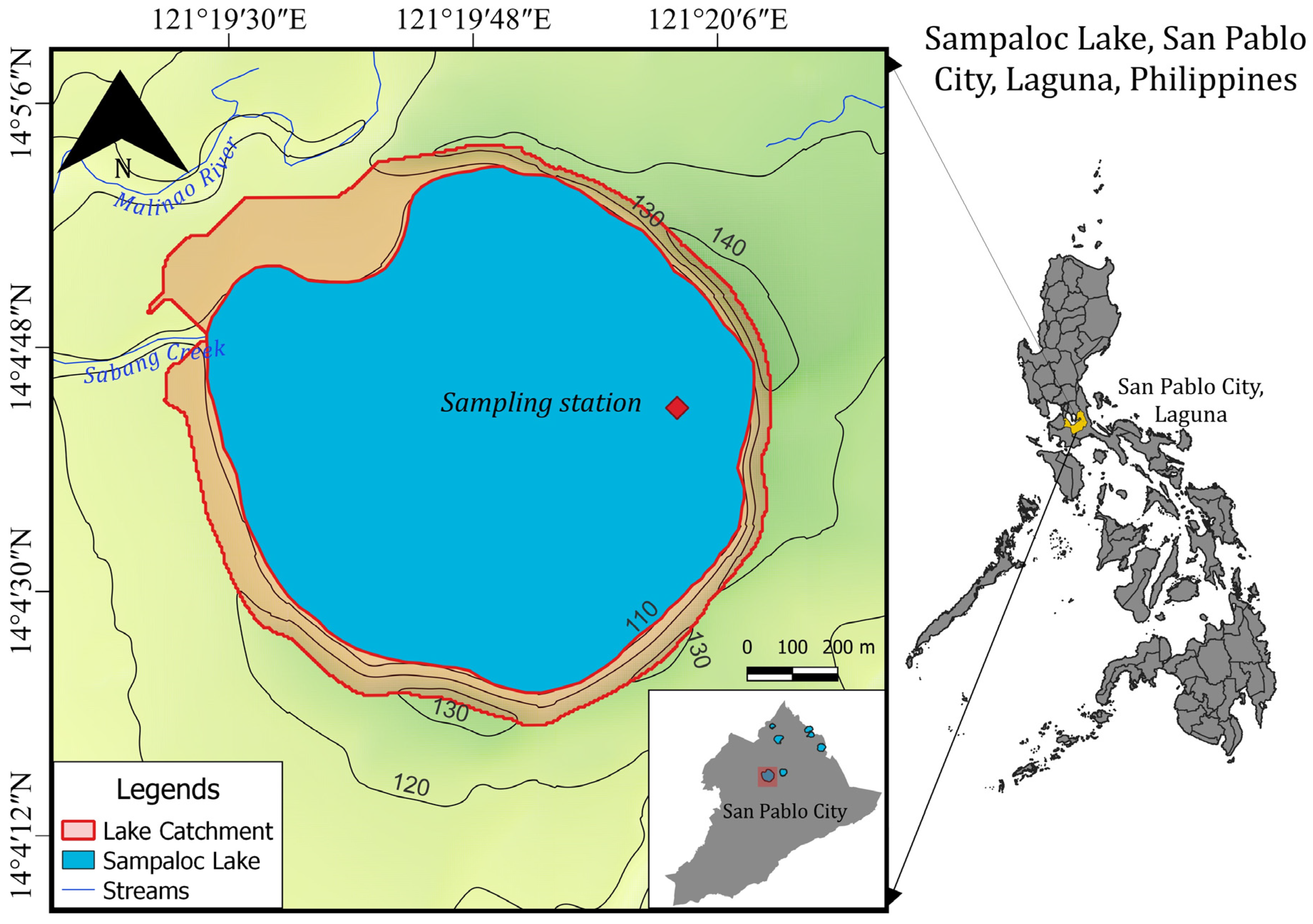
2.1. Site Background

Located at the center of San Pablo City, Laguna, Philippines, Sampaloc Lake (Figure 1) is the largest and premier lake among the six others in the area. The freshwater reservoir is of volcanic origin formed through a phreatic eruption when the lava from a nearby volcano reached the groundwater, causing an explosion resulting in a shallow depression [25]. Its circular shape is a feature like the other crater lakes in the city. The aquatic system obtains its water from various sources, including precipitation, runoff from the neighboring terrain, and numerous springs within the vicinity. The water within the reservoir is discharged through mechanisms such as soil seepage, evaporation, and outflow toward Sabang Creek, which serves as the lake’s sole water outlet [26].

Sampaloc Lake has a water surface area of 104 ha at an elevation of 106 m above mean sea level and its catchment area is relatively small at only 26 ha. With a mean depth of 20 m and a maximum depth of 27 m [27], its mixed layer has a water retention time of four years, indicating a slow rate of water volume exchange that leads to a stable stratification in the lake. The lake also supports various activities centered around ecotourism and aquaculture. Miniparks and boardwalks have been established around the lake and have become an attractive feature to visitors from various parts of the province [26]. Moreover, native and non-native aquatic species such as tilapia, silver perch, mudfish, and catfish bound the lake as they are used for commercial business by fisherfolks in the community [28]. Its rich biodiversity and cultural significance make it an appealing site for different research in biology and social sciences. However, studies particularly involving 3D hydrodynamic modeling remain limited. With its deep but small surface area and accessibility from the conducting institution, the lake is an ideal candidate for simulating water quality challenges and dynamics.

2.2. Field Measurement

Monthly field monitoring in the lake was made at the sampling station (Figure 1), situated at 14°04′42″ N and 121°20′03″ E. This is the same location where the country’s local limnological agency collects some of the lake’s water quality information at certain months of the year. Measurement was carried out with the use of a bamboo raft for navigation, as motorboats are prohibited in the field. Temperature measurements were made three times, once each month, from March to May 2023, between 10:00 and 12:00, under normal dry conditions. The multiparameter YSI Pro DSS was employed to measure various water quality parameters of the lake, including its temperature and depth profile. The instrument was submerged into the water at a consistent rate, recording different parameters every second.

2.3. Computation of Stratification Index

To quantitatively define the thermal structure of the reservoir, this study uses Brunt–Vaisala frequency (N²) as the measurement of the lake’s buoyancy and stability to vertical displacements such as those caused by convection [29]. It is given by the formula that follows:

$$N^2=-\frac{g \partial \rho }{\rho \partial z}$$

(1)

where N² (s⁻²) is computed on all measured layers in the lake based on the vertical density gradient $\frac{\mathrm{g}\delta \rho }{\rho \delta Z}$, where g (9.80 m s⁻²) is the acceleration due to gravity and $\rho$ (kg m⁻³) is the density at depth z (m). The value N² depends on the width of the thermocline and the lake’s stratification strength. A higher N² aligns with a steeper density gradient and thermocline within the lake. This index effectively measures the temperature gradient intensity in the lake, with a higher frequency observed within the metalimnion or the region of the thermocline.

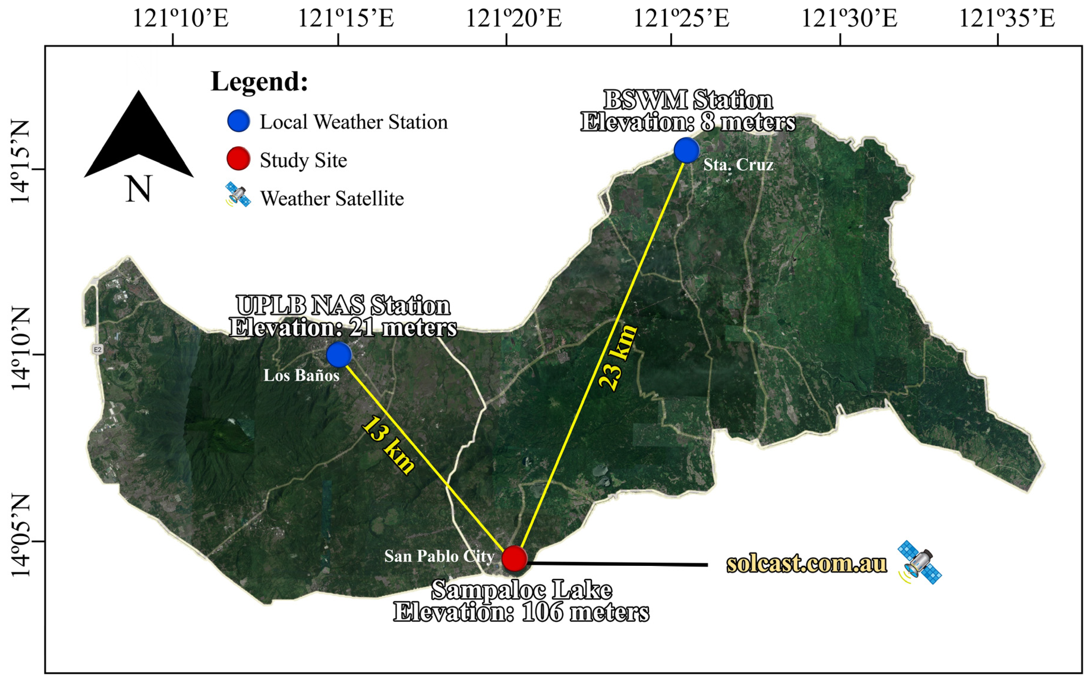
2.4. Weather Data Collection and Preliminary Analysis

Weather influences the heat transfer dynamics in environmental simulations [30]. Researchers focus on understanding the intricate relationship between weather parameters like temperature, wind speed, and solar radiation, and heat transfer in lakes [31,32]. For small stratified tropical lakes, local climate conditions, particularly air temperature and wind speed, affect the stratification of layers of the water body. Air temperature controls surface heat flux, influencing thermal convection initiation, while wind speed affects heat and momentum flux. Disruptions in surface heat flux can induce thermal convection in the water column. This phenomenon tends to be slower when compared to the overturns of lakes [33].

Two local weather stations, the University of the Philippines Los Baños National Agro-meteorological Station (UPLB NAS) and the Bureau of Soils and Water Management (BSWM), serve as primary sources of meteorological data within the area. The nearest weather station to the study site was the UPLB NAS (14°11′ N, 121°15′ E) located 13 km away, while the BSWM (14°16′ N, 121°24′ E) is farther at 23 km away (Figure 2). While these stations provide valuable information about the weather patterns and conditions in the region, neither of the two stations fulfill the requirements for input in the 3D model. UPLB NAS provides daily data rather than hourly. In addition, wind speed measurements were recorded at a height of 1 m above land surface, as opposed to the 10 m wind speed measurement requirement for Fantom Refined. Furthermore, the BSWM may have sub-daily data, but its most recent measurements, which are required for this paper, are unavailable. This led to the adoption of Solcast as a satellite-based weather data provider.

Solcast is a global online satellite data provider that offers live forecasts and historical weather data of twenty-seven weather parameters. These data are generated through eleven global weather satellites, capturing high-resolution and multi-spectral imagery with a monthly database update. Users can customize data intervals at 5, 10, 15, 30, or 60 min from 2007 to the present. The spatial resolution of the data averages around 1 to 2 km, excluding ocean and polar regions. Additionally, the reliability of the data is reinforced by peer-reviewed industry-standard models and algorithms, verified through a network of 70 global sites.

Compared to data from local stations, Solcast provides complete and latest hourly data that are suitable for 3D modeling input. However, integrating satellite data demands a certain validation approach to ensure its accuracy to actual meteorological conditions. To address this, this study utilized a simple correlation analysis, associating the existing daily datasets from the UPLB NAS and BSWM against those from Solcast. The analysis took place using complete available data from the most recent three years, with a focus on air temperature, wind speed, and solar radiation.

2.5. Numerical Simulation

2.5.1. Model Description

Shintani [24] developed a 3D numerical simulation tool known as Fantom Refined [4,15,34,35,36,37]. It is an open-source tool used in studies of temperate and subtropical reservoirs, as well as estuaries. With its versatility, it holds the potential for exploring tropical lakes and reservoirs. This model utilizes the three-dimensional Navier–Stokes equations with the assumption of incompressibility and the Boussinesq approximation

$$\frac{\partial u}{\partial t}+u\frac{\partial u}{\partial x}+v\frac{\partial u}{\partial y}+w\frac{\partial u}{\partial z}-fu=-\frac{1}{{\rho }_0}\frac{\partial p}{\partial x}+\frac{\partial }{\partial x}\left(v_H\frac{\partial u}{\partial x}\right)+\frac{\partial }{\partial y}\left(v_H\frac{\partial u}{\partial y}\right)+\frac{\partial }{\partial z}\left(v_V\frac{\partial u}{\partial z}\right)$$

(2)

$$\frac{\partial v}{\partial t}+u\frac{\partial v}{\partial x}+v\frac{\partial v}{\partial y}+w\frac{\partial v}{\partial z}-fv=-\frac{1}{{\rho }_0}\frac{\partial p}{\partial y}+\frac{\partial }{\partial x}\left(v_H\frac{\partial v}{\partial x}\right)+\frac{\partial }{\partial y}\left(v_H\frac{\partial v}{\partial y}\right)+\frac{\partial }{\partial z}\left(v_V\frac{\partial u}{\partial z}\right)$$

(3)

$$\frac{\partial w}{\partial t}+u\frac{\partial w}{\partial x}+v\frac{\partial w}{\partial y}+w\frac{\partial w}{\partial z}=-\frac{1}{{\rho }_0}\frac{\partial p}{\partial z}+\frac{\partial }{\partial x}\left(v_H\frac{\partial w}{\partial x}\right)+\frac{\partial }{\partial y}\left(v_H\frac{\partial w}{\partial y}\right)+\frac{\partial }{\partial z}\left(v_V\frac{\partial w}{\partial z}\right)-\frac{g}{{\rho }_0}\left({\rho }_0+\rho \right)$$

(4)

subject to incompressibility

$$\frac{\partial u}{\partial x}+\frac{\partial v}{\partial y}+\frac{\partial w}{\partial z}=0$$

(5)

where $u, v,$ and $w$ are the velocities in the $x, y,$ and $z$ directions, respectively. In addition, $p$ is the pressure, ${\rho }_0$ is the reference density, $\left({\rho }_0+\rho \right)$ is the density, $f(=2\mathsf{\Omega }sin\varphi )$ is the Coriolis coefficient, $\varphi$ is the latitude, and $\mathsf{\Omega }$ is the angular velocity of the Earth. Meanwhile, ${\nu }_H$ and ${\nu }_V$ are the horizontal and vertical eddy viscosity coefficients. The transport equation for temperature is calculated as follows:

$$\frac{\partial T}{\partial t}+u\frac{\partial T}{\partial x}+v\frac{\partial T}{\partial y}+w\frac{\partial T}{\partial z}=\frac{\partial }{\partial x}\left({\kappa }_H\frac{\partial T}{\partial x}\right)+\frac{\partial }{\partial y}\left({\kappa }_H\frac{\partial T}{\partial y}\right)+\frac{\partial }{\partial z}\left({\kappa }_V\frac{\partial T}{\partial z}\right)$$

(6)

where $T$ is the temperature and ${\kappa }_H$ and ${\kappa }_V$ are the horizontal and vertical eddy diffusion coefficients.

The equations were transformed into a discrete form using a collocated finite-volume approach. The second-order Adams–Bashfort method for explicit terms discretized the temporal derivatives, while, for the advection terms, the third-order ULTIMATE-QUICKEST scheme was used [38].

2.5.2. Heat Flux Boundaries

The net heat flux across air/water interface $Q_{net}$ is determined using

$${ Q}_{net}=Q_{Sn}+Q_L+Q_E+Q_C$$

(7)

The heat flux components, which include $Q_{Sn}$ for net shortwave solar radiation, $Q_L$ for longwave radiation flux, $Q_E$ for latent heat flux due to evaporation, and $Q_C$ for sensible heat flux due to conduction, were calculated based on air temperature, humidity, cloud cover, radiation, and wind speed using a bulk formula proposed by Kondo [39].

The integration of heat flux scaling factors improves the estimation of the lake’s thermal condition [12]. The calibrated scaling factors were added to the heat flux components, including shortwave, longwave, wind, and air temperature.

The net shortwave solar radiation flux is given by the Beer–Lambert law as follows:

$${ Q}_{Sn}=Q_{SR}{f}_{SW}\left(1-{\alpha }_{SW}\right){(1-e}^{K_{w}z})$$

(8)

where $Q_{SR}$ is measured solar radiation, $f_{SW}$ is a shortwave scaling factor, ${\alpha }_{SW}$ is shortwave albedo (0.07), and $K_w$ is the light extinction coefficient, expressed in units of m⁻¹. Users have the option to either set $K_w$ as a constant or associate it with the water quality model. The variable z represents the depth [17].

The net shortwave solar radiation flux was adjusted by integrating the longwave scaling factor, computed as

$$Q_L=\epsilon \sigma f_{LW}\left\{\left[9.37\times {10}^{-6}{\left(T_a+273.16\right)}^6\right]\left[1+.17C^2\right]-{\left(T+273.16\right)}^4\right\}$$

(9)

where $\epsilon$ is the emissivity of the water body (0.96), $\sigma$ is the Stefan–Boltzmann constant (=5.67 × 10⁻⁸ W m⁻² K⁻⁴), and $f_{LW}$ is a longwave scaling factor. $T$ is water temperature (°C), $T_a$ is atmospheric temperature (°C), and $C$ is the cloud fraction.

The wind scaling factor was applied to the latent heat flux due to evaporation, and is quantified by

$${ Q}_E=L_V{\rho }_a{U}_{10}{f}_W\left\{q_s-q_a\right\}$$

(10)

where $L_V$ represents the latent heat of the vaporization of water, ${\rho }_a$ is the density of air, $U_{10}$ is wind speed at 10 m above the surface, and $f_W$ is a wind scaling factor. The specific humidity of saturated air, denoted as $q_s$, is calculated by $q_s=\frac{0.622e_s}{P_{atm}-0.378e_s}$. Similarly, the specific humidity of remote air, referred as $q_a$, is determined by $q_a=\frac{0.622e_a}{P_{atm}-0.378e_a}$, with $e_s$ as the saturation vapor pressure and $e_a$ as the actual vapor pressure.

Lastly, both wind and air temperature scaling factors were integrated into the sensible heat flux due to conduction using the formula

$${ Q}_C={c_p\rho }_a{U}_{10}{f}_W\left\{T-T_a{f}_{AT}\right\}$$

(11)

where $c_P$ is the specific heat of air and $f_{AT}$ is an air temperature scaling factor.

2.6. Initial and Boundary Conditions

The temperature profiles from 25 March to 20 May 2023 from monthly field observations were used for validating the simulation results. Inflow, originating from the surrounding terrain, rainfall, and numerous local springs, was calculated using the rational method, a simple rainfall–runoff modeling technique. It was assumed that both inflow and outflow are constant, thus providing no significant change in the lake’s water level. Furthermore, the river temperature was calculated based on air temperature using a non-linear model proposed by Bautista [40] for a certain river in the Philippines.

$${ T}_w=\frac{31.40}{1+e^{0.14(15.24-T_a)}}$$

(12)

where $T_w$ is the water temperature.

For the weather data, hourly values of wind speed (m s⁻¹), wind direction (°), air temperature (°C), relative humidity (%), solar radiation (W m⁻²), atmospheric pressure (Pa), rainfall (mm), and cloud cover (%) were obtained from Solcast.

Uniform grids were set on the horizontal (dx = 80 m, dy = 80 m) and the vertical (dz = 0.5 m) axes. The time step, dt, was set at 10 s. The vertical temperature profile for March 25 was set as the initial condition.

2.7. Model Sensitivity and Calibration

Two approaches were implemented to fit actual data with the model. The first method involves the direct modification of weather parameters, including air temperature, solar radiation, and wind speed. The second one introduces scaling factors to the heat flux equations, which were described in Section 2.5.2. The latter is better than the former such that the implemented scaling factors do not compromise the integrity of the weather data.

Sensitivity analysis was initially carried out using the one-at-a-time (OAT) approach, where a single parameter varies while maintaining all other parameters as fixed at their initial values [41]. The results obtained from the sensitivity analysis were used as a basis in creating scaling factors systematically. This method of sensitivity analysis was utilized in several studies, including those involving generalized linear models (GLMs), as illustrated in

Table 1. Summary of scaling factors for tropical lakes [42,43].

Parameter	Description	Calibration Range
$f_{SW}$	scaling factor for solar radiation	0.7–1.3
$f_{LW}$	scaling factor for longwave radiation	0.7–1.3
$f_{AT}$	scaling factor for air temperature	0.7–1.3
$f_W$	scaling factor for wind	0.7–1.3

[42,43].

The normalized sensitivity index (SI) is quantified by

$$SI=\frac{\Delta Y/Y}{\Delta X/X}$$

(13)

where Y represents the model performance for the reference value X of the parameter, exhibiting a variation ΔX that generates a corresponding model performance variation ΔY [41]. A value of at least 0.07 is considered as sensitive for calibration. Meanwhile, the model performance is calculated as follows:

$$RMSE=\sqrt{\frac{{\sum }_{i=1}^N{(S_i-O_i)}^2}{N}}$$

(14)

where $N$ is the number of observations, whereas $S_i$ and $O_i$ refer to the “ith” simulated and observed data, respectively.

3. Results

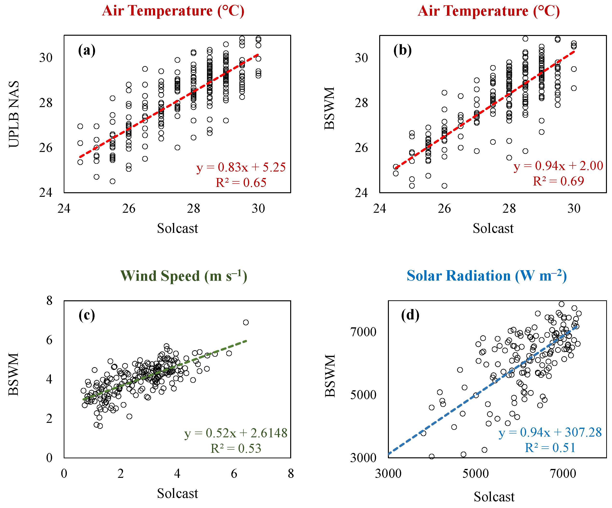
3.1. Weather Correlation

Satellite data validation with land-based observations is imperative for assessing the accuracy and reliability of atmospheric measurements over a small tropical lake [44]. In this study, an assessment of the relationship between Solcast and the UPLB NAS and BSWM was conducted to verify the remotely sensed data. Figure 3a correlates Solcast and UPLB NAS data, while Figure 3b,c provide the data correlations between Solcast and the BSWM. Bland [45] categorized R² values from the correlation analysis as follows: very weak correlation (0–0.19), weak correlation (0.20–0.39), moderate correlation (0.40–0.59), strong correlation (0.60–0.79), and very strong correlation (0.80–1.0). It can be seen in both Figure 3a,b that the correlation between the mean of the maximum and minimum daily air temperature yielded an R² of 0.65 and 0.69, respectively, indicating a strong correlation, while the mean daily wind speed in Figure 3c resulted in an R² of 0.53, suggesting a moderate correlation. Lastly, Figure 3d illustrates the correlation between the BSWM and Solcast for mean daily solar radiation, yielding an R² of 0.53, denoting a moderate correlation.

Overall, the mean of the maximum and minimum daily air temperature resulted in strong correlations. The moderate correlation for wind speed could be attributed to potentially localized weather conditions affecting wind patterns, which vary significantly due to factors like terrain and local topography [46]. Similarly, solar radiation resulting in moderate correlation might be influenced by variations in cloud cover and atmospheric conditions, as clouds can obstruct and disperse sunlight, leading to fluctuations in measurements [47]. Moreover, a comparative study conducted by Miri et al. [48] suggested that correlation coefficients exceeding 0.5 are acceptable for validating satellite-based systems against ground-based measurements, further supporting the acceptability of the 0.5 to 0.7 range.

Notably, the BSWM is located several kilometers in distance from the study site, while the Solcast satellite data were directly gathered at the study site location. This geographic proximity between the two meteorological sources potentially contributed to the disparities in observed solar radiation measurements. The findings indicate that Solcast data show an acceptable discrepancy compared to the ground-based measurements of the atmospheric conditions near Sampaloc Lake, therefore substantiating their reliability and accuracy.

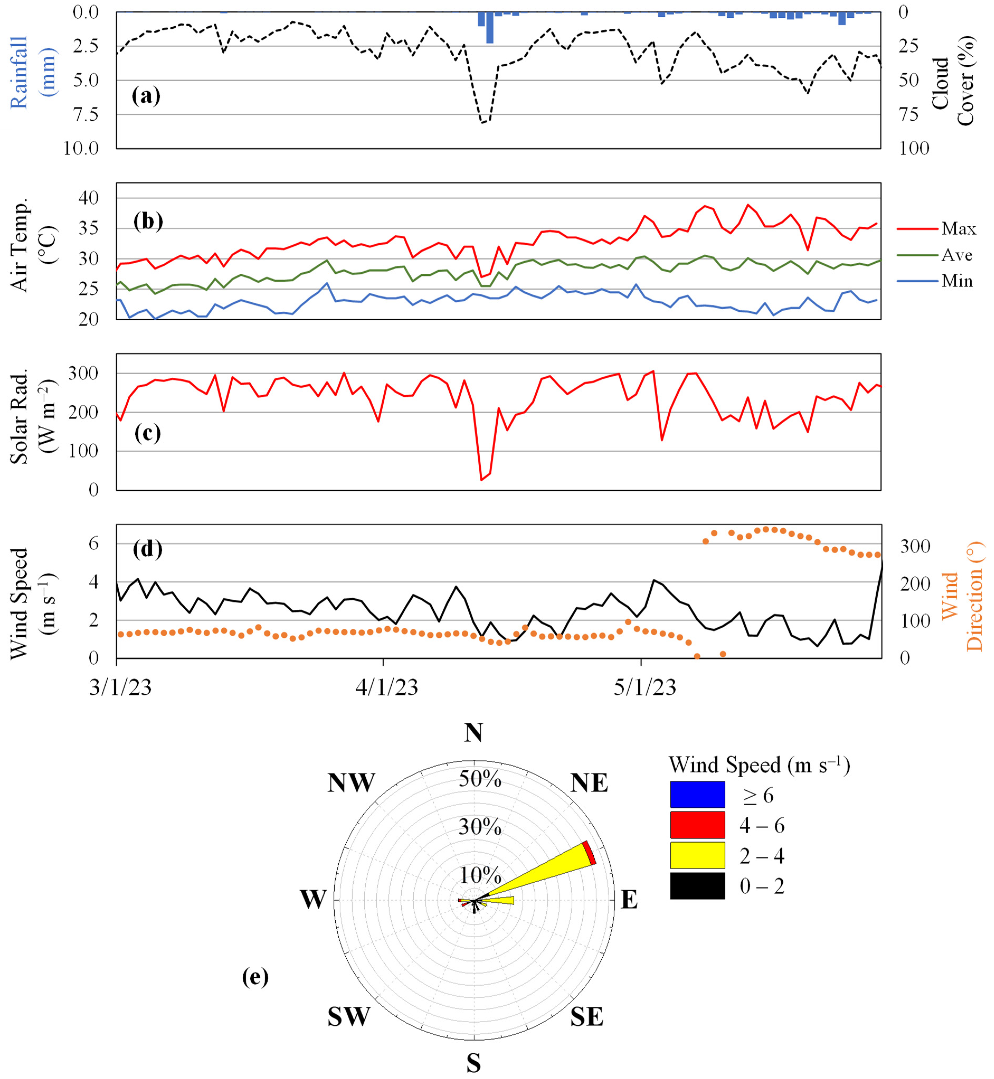
3.2. Meteorological Trends

Weather parameters, including rainfall, cloud cover, air temperature, solar radiation, wind direction, and wind speed, are presented in Figure 4 for the period from March to May 2023. Overall, the recorded rainfall (Figure 4a) during the time is minimal compared to the Philippines’ yearly average, attributable to the observation taking place during the country’s dry season. The average daily rainfall for the period is a mere 0.13 mm, with the first month being the driest and May the wettest, indicating a negligible effect of precipitation on the 3D modeling. There is no discernable impact from typhoons in the vicinity over the testing period, leading to a more stable stratification in the lake. Simultaneously, cloud cover averages 27%, with the sky becoming completely covered during some significant rainfall events.

For air temperature (Figure 4b), the monthly averages ranged from 24.3 to 30.5 °C. An observable upward trend in temperatures was noted as the weather transitioned from the previous colder months. In March, the minimum temperature reached its lowest at 20.1 °C, while its highest was at 26.0 °C. Conversely, the maximum temperature was 38.9 °C, which was observed in May. The direct correlation between high air temperature and the lake’s thermal stability is crucial, leading to a restricted mixing that hampers the replenishment of other water quality parameters in deeper waters [49].

For solar radiation (Figure 4c), the average daily energy output ranges from 26 W m⁻² to 305 W m⁻², with the highest mean value occurring in March and the lowest in May. The discernable pattern indicates a decrease in solar radiation received by the lake throughout the testing period. The interplay of solar radiation and air temperature can significantly influence the daily fluctuations in water temperature within the lake [50,51]. Additionally, these variations may be linked to cloud cover, which acts as a barrier to direct solar radiation, reducing the availability of light necessary for aquatic processes.

Wind speed (Figure 4d) plays a crucial role in the turnover and mixing of the lake. Among the other meteorological factors, it has the most significant impact on mixing [52]. During the monitoring period, the values of wind speed ranged from 0.7 to 5.8 m s⁻¹. Higher wind speeds are prevalent in March, with an average of 3 m s⁻¹. However, the trend proceeds to decline over time as it only averages 2.3 m s⁻¹ in May.

For wind direction (Figure 4d,e), the Northeast Monsoon is predominant at the start of the observation period, with the wind mainly coming from the East–Northeast direction. However, a shift in the wind pattern was observed before the end of May, indicating the end of the Northeast Monsoon, and marking the start of the Southwest Monsoon. Along with wind speed, the wind direction can be an indicator of a high concentration of different water quality parameters in the surface of the lake and can also act as a regulator of the physical environment since it can either disrupt or deepen the layer of stratification, depending on the morphology of the water body [53,54].

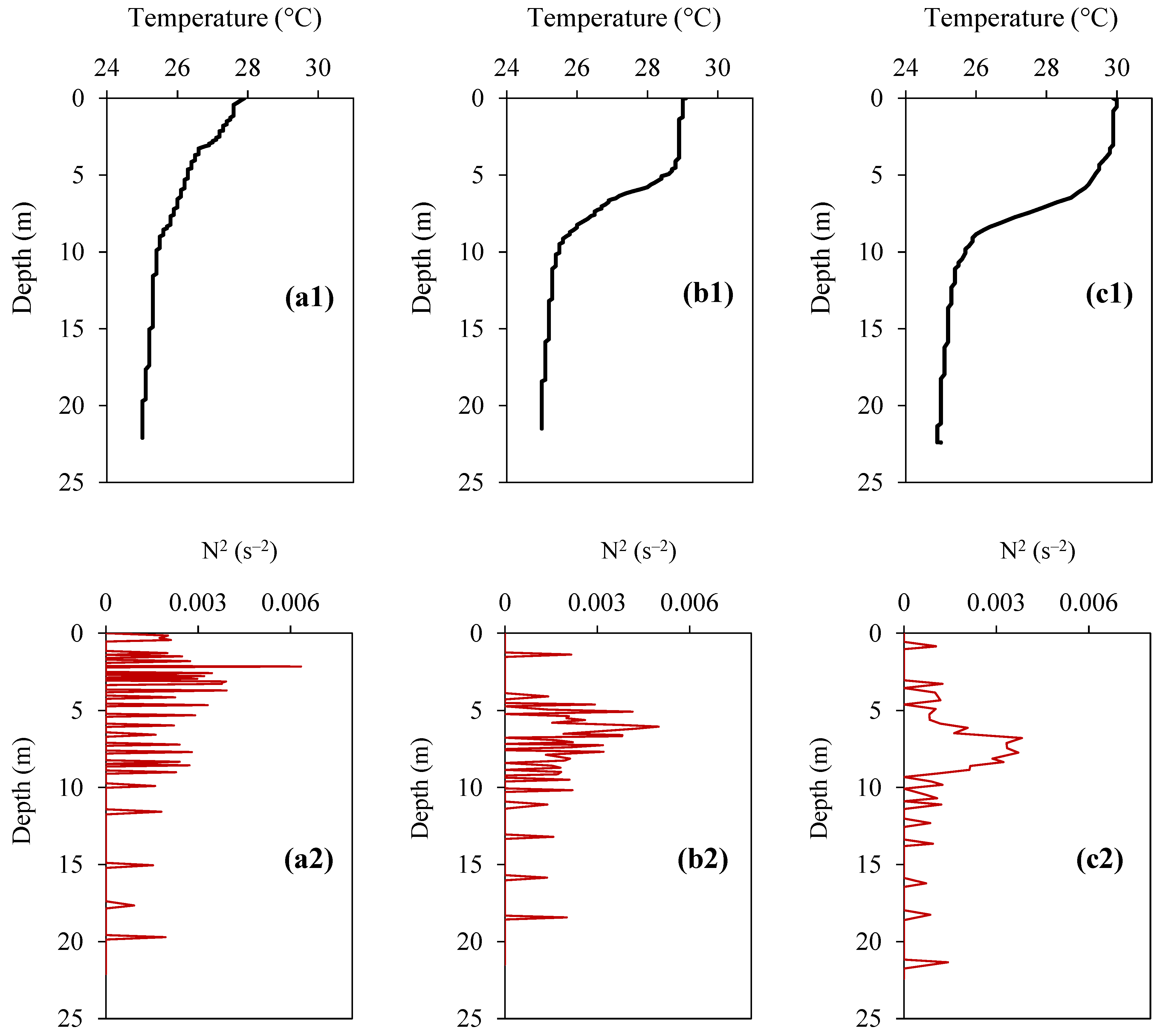
3.3. Thermal Structure of the Lake

The temporal variation in water temperature is provided in Figure 5. While the thermal profile remains stratified, the depth and thickness of the thermocline varies near the surface of the reservoir. A shallow and weak thermocline was observed in March (Figure 5a). This can be associated with the lake recovering from its natural mixing regime, which typically happens in the earlier months of the year [55]. In the next months, the increasing air temperature caused a higher lake temperature and a deeper and steeper thermocline. It was observed that the warmer epilimnion gradually thickens (Figure 5b,c), but the cooler hypolimnion remains the same at a temperature of 25 °C. Overall, the major changes for these times in the lake were only observed at the mixing layer of the lake, as the lake’s thermal structure attempts to stabilize for the rest of the year.

To quantify the resistance of the water column against turbulence and vertical displacement, the Brunt–Vaisala frequency (N²) was computed based on the density of the water body. The warming trend of the lake is notable, evident in the increasing running average of N². March (Figure 5a1,a2) exhibits the weakest stability during the three-month testing period, as the lake is still in the process of recovering from its cooled stage. Subsequently, the lake gains more heat in April (Figure 5b1,b2), coinciding with an increased frequency. May (Figure 5c1,c2) emerges as the month with the highest N², boasting the strongest thermocline over the three-month period. This occurrence aligns with minimal rainfall, reduced windspeed, and the concurrent rise in air temperature, leading to strong and defined lake stability.

4. Discussion

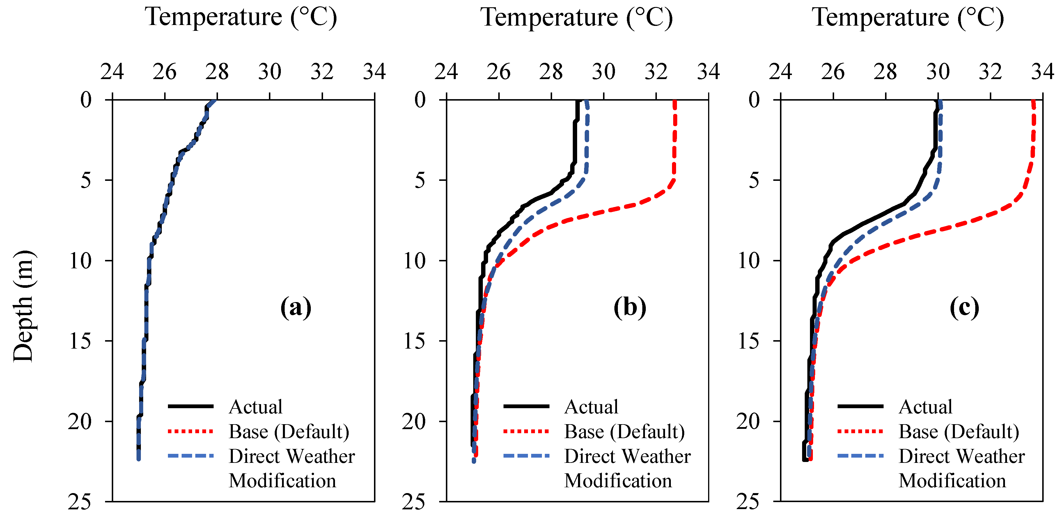
4.1. Preliminary Model Runs

4.1.1. Base Model Profiles Using Default Setting

Using Fantom Refined and its default parameters, the water temperature profile was simulated. In Figure 6, the simulated temperatures are compared with actual temperature data for the months of March, April, and May 2023. The root mean square error (RMSE), a widely used model evaluation statistic in similar hydrodynamic model studies [4,15,34,35,36,37], serves as a metric used to measure the agreement between the simulated results and the actual field data. During the initial model runs in March, no significant discrepancies emerged, as expected, given that this represents the model’s starting point (Figure 6a). However, in April and May, discrepancies between the actual and simulated results became evident. Specifically, in April, the RMSE values reached 10.41 °C (Figure 6b) and, in May, they increased to 11.69 °C (Figure 6c), indicating areas where potential improvements in the model’s performance are needed. These can be referred to in the “base” temperature profiles in red broken lines.

Among several hydrodynamic factors, one possible reason to consider is that the model was mostly tested for temperate and sub-tropical lakes. Considerable differences in environmental conditions occur between temperate and tropical regions [26]. Also, applying the model to small, stratified tropical lakes like the Sampaloc Lake necessitates specific adjustments to heat flux components. Factors such as shortwave, longwave, sensible, and latent heat fluxes, which vary significantly between temperate and tropical regions, play a role in these discrepancies and need to be considered for model enhancement.

Meteorological parameters are integral components influencing the heat flux equations used in hydrodynamic models like Fantom Refined [4,24,39]. These parameters include air temperature, solar radiation, and wind speed, considering the major atmospheric forcings affecting surface water systems [10]. An initial comparative analysis between the model’s simulations and the actual meteorological parameters (Figure 4) reveals a significant discrepancy in surface water temperature, deviating by approximately 3 to 4 °C from the air temperature. This may be attributed mainly to the configuration of the heat transfer model, which utilizes meteorological parameters such as air temperature, solar radiation, and wind speed. The wind field data produced by Solcast’s satellite can also be considered for modification due to possible topographical differences from land data. Consequently, adjustment to the current heat flux equations or the replacement of other heat flux models is essential to better replicate the observed data.

4.1.2. Model Profiles after Input Weather Modification

The pronounced impact of heat flux components, including air temperature, solar radiation, and wind speed, was observed previously on the modeled temperature profiles. The subsequent focus was on the direct modification of these parameters to optimize the model’s performance. Reduction coefficients were introduced to run different sensitivity analyses. The goal was to fine-tune the model, allowing it to replicate actual data more closely while minimizing the adjustments made to the meteorological parameters.

Through a series of case analyses with varying reduction coefficients applied to air temperature, solar radiation, and wind speed, the model results gradually approached a closer match with the actual temperature values as seen in Figure 6. Remarkably, the reduction coefficients of 2 °C for air temperature, 40% for solar radiation, and 50% for wind speed yielded the best alignment between model outputs and observed data. These can be referred to in the “adjusted” temperature profile in blue broken lines.

In terms of the RMSE, these adjustments resulted in significant improvements. The initial RMSE value of 10.41 °C for April decreased to 2.37 °C, while the May value of 11.69 °C was reduced to 2.13 °C. It becomes evident that these reduction coefficients reflect the substantial influence of air temperature, solar radiation, and wind speed on the heat flux equations used in the hydrodynamic model. While these optimizations improve the accuracy of the model’s output, they also introduce a trade-off between closely representing the simulated data and maintaining the integrity of the original weather data inputs.

4.2. Application of Heat Flux Scaling Factors

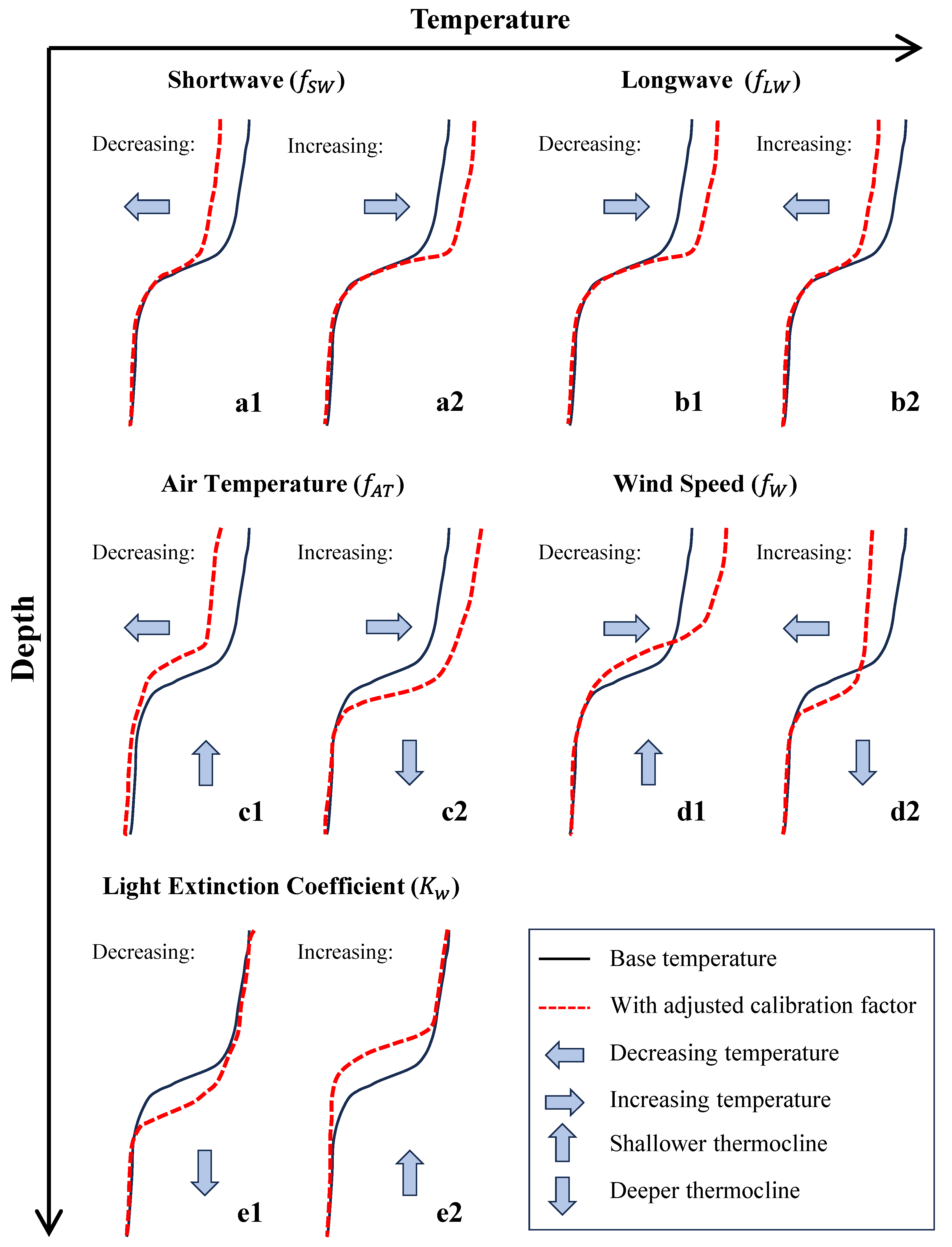
4.2.1. Sensitivity Analysis and Trend

Table 2. Model performance (Y) and sensitivity index (SI) of selected heat flux parameters using OAT approach. SI > 0.07 was declared as sensitive and calibrated.

Parameter (Factor)	Parameter Value (X)			Model Performance (Y)			Sensitivity Index (SI)
	Initial	Lower	Upper	Initial	Lower	Upper	Lower	Upper	Average
$f_{SW}$	1.00	0.70	0.90	6.75	5.20	6.00	0.57	1.12	0.85
$f_{LW}$	1.00	0.70	0.90	6.75	3.78	5.89	1.47	1.28	1.37
$f_{AT}$	1.00	0.70	0.90	6.75	4.65	6.06	1.04	1.03	1.04
$f_W$	1.00	0.70	0.90	6.75	8.20	7.04	0.43	0.43	0.43

shows the model performance and sensitivity analysis of selected heat flux parameters of Fantom Refined. Using the OAT method, the factors with the strongest to least sensitivities are longwave (SI = 1.37), air temperature (SI = 1.04), shortwave (SI = 0.85), and wind (SI = 0.43), respectively. Having a higher SI implies that even a slight adjustment in the value corresponds to a significant effect on the thermal profile. All selected parameters were identified as sensitive and were calibrated in subsequent procedures. Also, Figure 7 illustrates the trends of the temperature profile in relation to modifying each factor. Decreasing the shortwave factor also decreases the temperature of the upper layer (epilimnion) of the lake and vice versa. However, an opposite trend is observed for the longwave factor as reducing the coefficient leads to an increased water temperature. These two factors generally affect the horizontal movement of the upper layer of the modeled profile. Moreover, air temperature and wind factors affect the upper portion and depth of the thermocline simultaneously. Decreasing the value of the air temperature factor also reduces the temperature of the mixing layer and its thermocline depth. On the other hand, reducing the wind factor increases the water surface temperature and makes the thermocline depth shallower. Additionally, it is observed that the susceptibility of the thermocline movement weakens as both the air temperature and wind factor reach lower values of 0.8 and below.

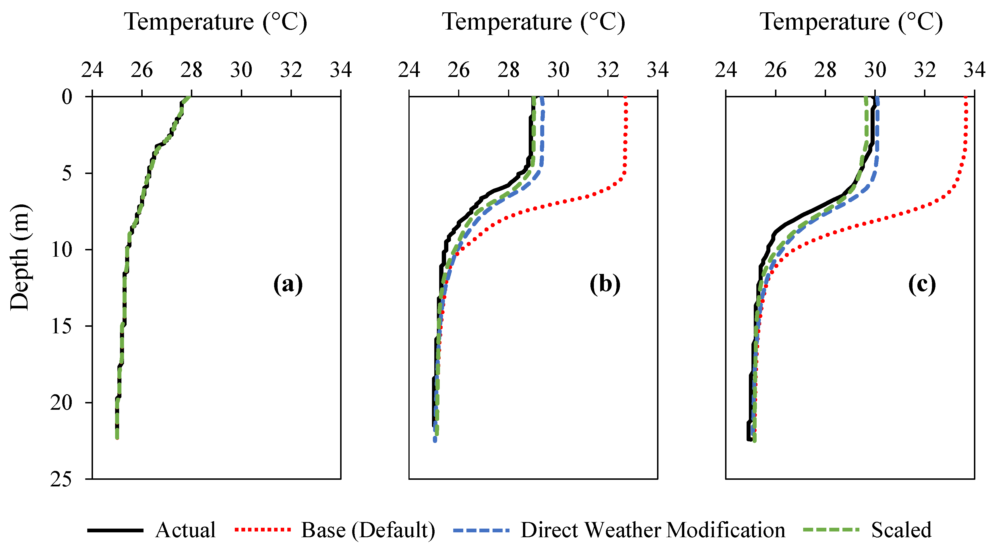
4.2.2. Final Model Profiles

After applying the heat flux factors, the model produced more reasonable temperature profiles. Factors multiplied to the following heat flux components: shortwave (0.75), longwave (1.35), air temperature (0.935), and wind (0.80). Monthly calibrated profiles (green) of March to May 2023, in comparison to the adjusted (blue), base (red), and actual temperature (black) profiles, are shown in Figure 8. Scaling factors yielded improved RMSE values from 2.37 °C to 1.32 °C and from 2.13 °C to 0.70 °C for the months of April (Figure 8b) and May (Figure 8c), respectively. Also, scaling factors are more flexible than manually adjusting the weather data. However, the adjustments in the four initial parameters are not enough to generate better results; thus, the adjustment in the light extinction coefficient $K_w$ was introduced. The light extinction coefficient indicates how quickly light diminishes as it travels through the water and is affected by the substances in the water. A higher coefficient is associated with a lower heat content in the water body [56]. Measurements of the Secchi depth [57], the depth from the water surface to the disk, can be related to the light extinction coefficient by

$$K_w=\frac{1.7}{Secchi Depth}$$

(15)

The $K_w$ for the months of September and December 2023 was 0.34 and 0.85, respectively, indicating that $K_w$ is temporally changing.

The calibration of the light extinction coefficient improves as it significantly affects the thermocline depth (Figure 7). Applying calibration factors produces acceptable results and ensures the integrity of the input weather data of the model, such as air temperature and wind.

4.3. Challenges to 3D Modeling of a Tropical Lake

Tropical lakes, located particularly in developing countries such as Southeast Asia, are provided little to no attention in terms of 3D hydrodynamic modeling due to several reasons. In this region, limnologic data are limited by the infrequent monitoring of the physical, chemical, and biological status of lakes. In the Philippines, only the major lakes such as the Laguna Lake and Taal Lake are monitored due to their large contribution to aquaculture industry. Small lakes such as the Sampaloc Lake are often not given the same priority. Without basic information such as consistent measurements of temperature profiles and other water quality parameters, the application of 3D modeling will fail without proper validation procedures. In this study, the temperature of the lake was monitored monthly for the year 2023, and these data served as the reference for the calibration and validation of the hydrodynamic model. This paper thus emphasizes the need to consistently monitor the water quality of lakes and reservoirs in the region.

Hydrologic information such as streamflow and river temperature are also lacking. For small lakes where catchments are also small, inflows into the lake can be estimated directly from rainfall using the rational method for streams without flow gauging stations. However, these flow values should be checked from time to time by performing actual flow measurement in these streams. In this study, the low and high flows generated from the rational method were counterchecked with the actual flow measurements in the tributary of Sampaloc Lake during dry and rainy periods. Also, one large component in modeling the lake’s thermal structure is the stream temperature, which also lacks information. While the Philippines may have daily monitoring of streamflow for major rivers in the country, the daily temperature and water quality of streams are barely available. This then resulted in the study adopting an existing regression model of river water temperature as a function of air temperature.

Weather information, in hourly or smaller intervals, is necessary for 3D hydrodynamic modeling that utilizes time steps as small as 10 s. While Sampaloc Lake has a nearby weather station (UPLB NAS), the data available are daily, not hourly. The other station may have sub-daily data (BSWM), but records are fragmentary and up-to-date information required for modeling for this study is unavailable, as this weather station has terminated operation. However, with the presence of satellite data from Solcast, the 3D modeling for Sampaloc Lake could proceed, as Solcast offers complete hourly weather information. However, satellite weather data should be used with caution by ensuring that they represent actual weather conditions. For this purpose, this study employed a simple correlation analysis of existing data from the UPLB NAS and BSWM with those of Solcast, and the results were proven to be acceptable.

Another factor that the modeler should look further into is the proper calibration of the model. As Fantom Refined was mostly used for temperate and subtropical lakes and reservoirs, this study found that using the default parameters of the model tends to overestimate the temperature of the tropical Sampaloc Lake. Hence, this paper introduces adjustments in calibration factors and light extinction in the heat flux components. In future, other heat flux equations other than from Kondo [39] will be tested for longer datasets and the addition of other scaling factors will be employed in conjunction with the use of 1D hydrodynamic modeling, such as the general lake model (GLM). Moreover, expanding the modeling period, perhaps to a year, would offer a thorough understanding of the lake’s temperature patterns and provide insights into its long-term dynamics and seasonal variations.

This paper outlines the challenges posed by performing 3D hydrodynamic modeling in a small tropical lake. This study pioneers this approach so that other researchers may be given a reference and direction in their future endeavors when carrying out 3D modeling for this region. Other matters that need to be considered are the lake water level monitoring as well as the production of reasonable and updated bathymetric data for the 3D modeling to properly proceed.

5. Conclusions

A pioneering study carried out 3D hydrodynamic modeling using Fantom Refined with a focus on temperature simulation for a small, stratified tropical lake in the Philippines. In this region, hydro-meteorological and limnological data are usually not easily accessible. Monthly monitoring of the lake’s temperature was conducted from March to May 2023, which served as the initial condition and point for the validation of the model. Meteorological data were taken from the Solcast website, providing hourly satellite weather data, which were duly validated using two local weather stations. Inflows were generated using the simple rainfall–runoff model while streamflow temperatures were estimated from a regression model where air temperature is the input. The combined satellite data and runoff model can therefore be utilized for 3D hydrodynamic modeling. As Fantom Refined was usually applied to temperate and sub-tropical lakes and reservoirs, the resulting temperature profiles using default parameters were warmer than those observed for tropical settings. This study initially opted to make some reductions to air temperature, solar radiation, and windspeed as a preliminary step in adjusting the heat flux components. However, the process compromised the integrity of the primary weather data. The calibration process was then employed by multiplying factors to components like shortwave (0.75), longwave (1.35), air temperature (0.935), and wind (0.80), including the adjustment light extinction coefficient (0.65). This underscores the importance of gathering actual field data for temperature for model validation purposes. This study identifies challenges in 3D hydrodynamic modeling for tropical lakes, such as paucity in input hydro-meteorological and limnological data and the need for the improvement of calibration factors for the heat flux models for tropical regions. It is recommended to continue gathering field data of temperature and water quality profiles in the lake as a basis to further improve the model. Overall, this study was successful in employing 3D hydrodynamic modeling in a tropical lake, which can pave directions for future modeling in the same region.

References

1. Zamani, B.; Koch, M. Comparison between two hydrodynamic models in simulating physical processes of a reservoir with complex morphology. Water 2020, 12, 814. [Google Scholar] [CrossRef]
2. Catalan, J.; Rondón, J. Perspectives for an integrated understanding of tropical and temperate high-mountain lakes. J. Limnol. 2016, 75, 216–234. [Google Scholar] [CrossRef]
3. Caramatti, I.; Peeters, F.; Hamilton, D.; Hofmann, H. Modelling inter-annual and spatial variability of ice cover in a temperate lake with complex morphology. Hydrol. Process. 2020, 34, 691–704. [Google Scholar] [CrossRef]
4. Duka, M.A.; Shintani, T.; Yokoyama, K. Thermal stratification responses of a monomictic reservoir under different seasons and operation schemes. Sci. Total Environ. 2020, 767, 144423. [Google Scholar] [CrossRef]
5. Bueche, T.; Hamilton, D.P.; Vetter, M. Using the general lake model (GLM) to simulate water temperatures and ice cover of a medium-sized lake: A case study of lake Ammersee, Germany. Environ. Earth Sci. 2017, 76, 461. [Google Scholar] [CrossRef]
6. Herrera, E.; Nadaoka, K.; Blanco, A.; Hernandez, E. Hydrodynamic investigation of a shallow tropical lake environment (Laguna Lake, Philippines) and associated implications for eutrophic vulnerability. Asean Eng. J. 2015, 4, 48. [Google Scholar]
7. Hodges, B.R.; Imberger, J.; Laval, B.E. Modeling the hydrodynamics of stratified lakes. Hydroinformatics 2000. Available online: https://www.researchgate.net/publication/255596842_Modeling_the_Hydrodynamics_of_Stratified_Lakes (accessed on 5 November 2023).
8. Ishikawa, M.; Gonzalez, W.; Golyjeswski, O.; Sales, G.; Rigotti, J.A.; Bleninger, T.; Mannich, M.; Lorke, A. Effects of dimensionality on the performance of hydrodynamic models for stratified lakes and reservoirs. Geosci. Model Dev. 2022, 15, 2197–2220. [Google Scholar] [CrossRef]
9. Heddam, S.; Ptak, P.; Zhu, S. Modelling of daily lake surface water temperature from air temperature: Extremely randomized trees (ERT) versus Air2Water, MARS, M5Tree, RF and MLPNN. J. Hydrol. 2020, 588, 125130. [Google Scholar] [CrossRef]
10. Ji, Z.G. Hydrodynamics and Water Quality: Modeling Rivers, Lakes, and Estuaries; John Wiley & Sons: Hoboken, NJ, USA, 2017. [Google Scholar]
11. Zhao, L.; Cheng, S.; Sun, Y.; Zou, R.; Ma, W.; Zhou, Q.; Liu, Y. Thermal mixing of Lake Erhai (Southwest China) induced by bottom heat transfer: Evidence based on observations and CE-QUAL-W2 model simulations. J. Hydrol. 2021, 603, 126973. [Google Scholar] [CrossRef]
12. Rahaghi, A.I.; Lemmin, U.; Cimatoribus, A.; Bouffard, D.; Riffler, M.; Wunderle, S.; Barry, D. Improving surface heat flux estimation for a large lake through model optimization and two-point calibration: The case of Lake Geneva. Limnol. Oceanogr. Methods 2018, 16, 576–593. [Google Scholar] [CrossRef]
13. Abed-Zaid, D.S.; Al-Zubaidi HA, M. Surface heat budget estimation for Laurance Lake, US. IOP Conf. Ser.Earth Environ. Sci. 2021, 877, 012005. [Google Scholar] [CrossRef]
14. Tomita, H.; Kutsuwada, K.; Kubota, M.; Hihara, T. Advances in the estimation of global surface net heat flux based on satelilite observation: J-OFURO3 v1.1. Fron. Mar. Sci. 2021, 8, 612361. [Google Scholar] [CrossRef]
15. Duka, M.A.; Iguchi, K.; Yokoyama, K.; Koizumi, A. Effect of selective withdrawal and vertical curtain on turbid water flow after a flood event in the Ogouchi Reservoir—Field Observation and 3D Numerical Simulation. In Proceedings of Japan Water Works Association; Japan Water Works Association: Tokyo, Japan, 2020. [Google Scholar]
16. Soulignac, F.; Vinçon-Leite, B.; Lemaire, B.J.; Scarati Martins, J.R.; Bonhomme, C.; Dubois, P.; Mezemate, Y.; Tchiguirinskaia, I.; Schertzer, D.; Tassin, B. Performance assessment of a 3D hydrodynamic model using high temporal resolution measurements in a shallow urban lake. Environ. Model. Assess. 2017, 22, 309–322. [Google Scholar] [CrossRef]
17. Hipsey, M.R.; Bruce, L.C.; Hamilton, D.P. General Lake Model: Model Overview and User Information; AED Report #26; The University of Western Australia: Perth, Australia, 2014; p. 42. ISBN 878-1-7-74052-303-5. [Google Scholar]
18. DHI Mike 21 & Mike 3 Flow Model FM—Hydrodynamic and Transport Module: Scientific Documentation. 2017. Available online: https://manuals.mikepoweredbydhi.help/2017/Coast_and_Sea/MIKE_321_FM_Scientific_Doc.pdf (accessed on 5 November 2023).
19. Octavio KA, H.; Jirka, G.H.; Harleman DR, F. Vertical heat transport mechanisms in lakes and reservoirs. Mass. Inst. Technol. Technol. Rep. 1977, 22. Available online: http://hdl.handle.net/1721.1/52844 (accessed on 5 November 2023).
20. Sweers, H.E. A nomogram to estimate the heat exchange coefficient at the air-water interface as a function of windspeed and temperature; a critical survey of some literature. J. Hydrol. 1976, 30, 375–401. [Google Scholar] [CrossRef]
21. Murakami, M.; Oonisishi, Y.; Kunishi, H. A numerical simulation of the distribution of water temperature and salinity in the Setol Inland Sea. J. Oceanogr. Soc. Jpn. 1985, 41, 221–224. Available online: https://api.semanticscholar.org/CorpusID:129568759 (accessed on 5 November 2023). [CrossRef]
22. Gill, A.E. Atmosphere-Ocean Dynamics; International Geophysics Series; Academic Press: Cambridge, MA, USA, 1982; p. 30. Available online: https://books.google.com/books?hl=en&lr=&id=1WLNX_lfRp8C&oi=fnd&pg=PR11&dq=Gill.+A.+E.+(1982).+Atmosphere-ocean+dynamics.+International+Geophysics+Series,+Academic+Press,+30.+&ots=Tr7337UWdP&sig=AINTdr3i7WF6tWbHe7tz0h9wpSI (accessed on 7 November 2023).
23. Lane, A. The Heat Balance of the North SEA; Technical Report #8; Proudman Oceanographic Laboratory: Liverpool, UK, 1989. [Google Scholar]
24. Shintani, T. An unstructured-cartesian hydrodynamic simulator with local mesh refinement technique. J. JSCE 2017, 73, 967–972. [Google Scholar] [CrossRef] [PubMed]
25. Gayllo, V.; Paller, V.; Magcale-Macandog, D.; Ryan, E.; De Chavez, C.; Grace, M.; Paraso, V.; Claret, M.; Tsuchiya, L.; Campang, J.; et al. The Seven Lakes of San Pablo: Assessment and Monitoring Strategies Toward Sustainable Lake Ecosystems. Philipp. Sci. Lett. 2021, 14. Available online: https://scienggj.org/2021/PSL%202021-vol14-no01-p158-179-Paller%20et%20al.pdf (accessed on 7 November 2023).
26. Brillo, B.B.C. Urban lake governance and development in the Philippines: The case of Sampaloc lake, San Pablo City. Taiwan Water Conserv. J. 2016, 64, 66–81. Available online: https://ssrn.com/abstract=2848705 (accessed on 5 November 2023).
27. de la Cruz, C.P.P.; Bandal, M.Z.; Avila, A.R.B., Jr.; Paller, V.G.V. Distribution pattern of Acanthogyrus sp. (acanthocephala: Quadrigyridae) in Nile tilapia (Oreochromis niloticus L.) from Sampaloc lake, Philippines. J. Nat. Stud. 2013, 12, 1–10. [Google Scholar]
28. LLDA Seven (7) Crater Lakes. 2014. Available online: https://llda.gov.ph/seven-7-crater-lakes/ (accessed on 15 November 2023).
29. Duka, M.A.; Shintani, T.; Yokoyama, K. Mediating the effects of climate on the temperature and thermal structure of a monomictic reservoir through use of hydraulic facilities. Water 2021, 13, 1128. [Google Scholar] [CrossRef]
30. Woolway, R.I.; Verburg, P.; Lenters, J.D.; Merchant, C.J.; Hamilton, D.P.; Brookes, J.; de Eyto, E.; Kelly, S.; Healey, N.C.; Hook, S.; et al. Geographic and temporal variations in turbulent heat loss from lakes: A global analysis across 45 lakes. Limnol. Oceanogr. 2018, 63, 2436–2449. [Google Scholar] [CrossRef]
31. Abbasi, A.; Annor, F.; Van de Giesen, N. Investigation of temperature dynamics in small and shallow reservoirs, case study: Lake Binaba, upper east region of Ghana. Water 2016, 8, 84. [Google Scholar] [CrossRef]
32. Guo, M.; Zhuang, Q.; Yao, H.; Małgorzata Gołub, L.; Leung, R.; Pierson, D.; Tan, Z. Validation and Sensitivity Analysis of a 1-D Lake Model Across Global Lakes. J. Geophys. Res. Atmos. 2021, 126, e2020JD033417. [Google Scholar] [CrossRef]
33. Pu, T. Stratification Stability of Tropical Lakes and Their Responses to Climatic Changes: Lake Towuti (Indonesia). 2023. Available online: https://www.proquest.com/docview/2784390988?pq-origsite=gscholar&fromopenview=true (accessed on 14 December 2023).
34. Duka, M.A.; Yokoyama, K.; Shintani, T.; Iguchi, K. Effect of selective withdrawal and vertical curtain on reservoir sedimentation: A 3-D numerical modeling approach. In River, Coastal and Estuarine Morphodynamics, Auckland, New Zealand. 2019. Available online: https://www.researchgate.net/publication/342826574_Effect_of_Selective_Withdrawal_and_Vertical_Curtain_on_Reservoir_Sedimentation_a_3-D_Numerical_Modeling_Approach?channel=doi&linkId=5f07d22c92851c52d62686a0&showFulltext=true (accessed on 5 November 2023).
35. Duka, M.A.; Yokoyama, K.; Shintani, T.; Iguchi, K.; Iwasaki, H.; Ueno, T.; Chiba, T. Influence of water control facilities on thermal stratification of Ogouchi Reservoir for 58 years. J. Jpn. Soc. Civ. Eng. Ser. B1 Hydraul. Eng. 2019, 75, 685–690. [Google Scholar] [CrossRef] [PubMed]
36. Duka, M.A.; Yokoyama, K.; Shintani, T.; Sakai, H.; Koizumi, A. Application of the modified Gaussian distribution method to reproduce the water temperatures of the Ogouchi Reservoir. J. JSCE Ser. B1 Hydraul. Eng. 2021, 77, I961–I966. [Google Scholar] [CrossRef]
37. Somsook, K.; Olap, N.A.; Duka, M.A.; Veerapaga, N.; Shintani, T.; Yokoyama, K. Analysis of interaction between morphology and flow structure in a meandering macro-tidal estuary using 3-D hydrodynamic modeling. Estuar. Coast. Shelf Sci. 2022, 264, 107687. [Google Scholar] [CrossRef]
38. Leonard, B.P. The ULTIMATE conservative difference scheme applied to unsteady one-dimensional advection. Comput. Methods Appl. Mech. Eng. 1991, 88, 17–74. [Google Scholar] [CrossRef]
39. Kondo, J. Air-sea bulk transfer coefficients in diabatic conditions. Bound. Layer Meteorol. 1975, 9, 91–112. [Google Scholar] [CrossRef]
40. Bautista PM, O. Modeling River Water Temperature from Air Temperature for Selected Rivers. University of the Philippines Los Banos, Los Baños, Philippines, 2022, unpublished undergraduate thesis. [Google Scholar]
41. Hamby, D.M. A review of techniques for parameter sensitivity analysis of environmental models. Env. Monit Assess 1994, 32, 135–154. [Google Scholar] [CrossRef]
42. Soares, L.M.; Calijuri, M.D.; Silva, T.F.; Novo, E.; Cairo, C.T.; Barbosa, C.C. A parameterization strategy for hydrodynamic modelling of a cascade of poorly monitored reservoirs in Brazil. Environ. Model. Softw. 2020, 134, 104803. [Google Scholar] [CrossRef]
43. Calamita, E.; Vanzo, D.; Wehrli, B.; Schmid, M. Lake Modeling Reveals Management Opportunities for Improving Water Quality Downstream of Transboundary Tropical Dams. Water Resour. Res. 2021, 57, e2020WR027465. [Google Scholar] [CrossRef]
44. Dinku, T.; Funk, C.; Peterson, P.; Maidment, R.; Tadesse, T.; Gadain, H.; Ceccato, P. Validation of the CHIRPS satellite rainfall estimates over eastern Africa. Q. J. R. Meteorol. Soc. 2018, 144, 292–312. [Google Scholar] [CrossRef]
45. Bland, M. Correlation and regression. In Statistics at Square One; BMJ Publishing Group Ltd.: London, UK, 2016; Available online: https://www.bmj.com/about-bmj/resources-readers/publications/statistics-square-one/11-correlation-and-regression (accessed on 3 January 2024).
46. He, Y.; Pak Wai, C.h.a.n.; Li, Q. Wind characteristics over different terrains. J. Wind Eng. Ind. Aerodyn. 2013, 120, 51–69. [Google Scholar] [CrossRef]
47. Zagouras, A.; Kazantzidis, A.; Nikitidou, E.; Argiriou, A.A. Determination of measuring sites for solar irradiance, based on cluster analysis of satellite-derived cloud estimations. Sol. Energy 2013, 97, 1–11. [Google Scholar] [CrossRef]
48. Miri, M.; Masoudi, R.; Raziei, T. Performance Evaluation of Three Satellites-Based Precipitation Data Sets Over Iran. J. Indian Soc. Remote Sens. 2019, 47, 2073–2084. [Google Scholar] [CrossRef]
49. Shinohara, R.; Tanaka, Y.; Kanno, A.; Matsushige, K. Relative impacts of increases of solar radiation and air temperature on the temperature of surface water in a shallow, eutrophic lake. Hydrol. Res. 2021, 52, 916–926. [Google Scholar] [CrossRef]
50. Rogora, M.; Buzzi, F.; Dresti, C.; Leoni, B.; Lepori, F.; Mosello, R.; Patelli, M.; Salmaso, N. Climatic effects on vertical mixing and deep-water oxygen content in the subalpine lakes in Italy. Hydrobiologia 2018, 824, 33–50. [Google Scholar] [CrossRef]
51. Yang, K.; Yu, Z.; Luo, Y. Analysis on driving factors of lake surface water temperature for major lakes in Yunnan-Guizhou Plateau. Water Res. 2020, 184, 116018. [Google Scholar] [CrossRef]
52. Zhou, J.; Yoshida, T.; Kitazawa, D. Numerical analysis of the relationship between mixing regime, nutrient status, and climatic variables in Lake Biwa. Sci. Rep. 2022, 12, 19691. [Google Scholar] [CrossRef] [PubMed]
53. Donis, D.; Mantzouki, E.; McGinnis, D.F.; Vachon, D.; Gallego, I.; Grossart, H.P.; de Senerpont Domis, L.N.; Teurlincx, S.; Seelen, L.; Lürling, M.; et al. Stratification strength and light climate explain variation in chlorophyll a at the continental scale in a European multilake survey in a heatwave summer. Limnol. Oceanogr. 2021, 66, 4314–4333. [Google Scholar] [CrossRef]
54. Zhang, W.; Xu, Q.; Wang, X.; Hu, X.; Wang, C.; Pang, Y.; Hu, Y.; Zhao, Y.; Zhao, X. Spatiotemporal distribution of eutrophication in Lake Tai as affected by wind. Water 2017, 9, 200. [Google Scholar] [CrossRef]
55. Aguilar, J.I.; Mendoza-Pascual, M.U.; Padilla KS, A.R.; Papa RD, S.; Okuda, N. Mixing regimes in a cluster of seven maar lakes in tropical monsoon Asia. Inland Waters 2023, 13, 47–61. [Google Scholar] [CrossRef]
56. Pal, S.; Das, D.; Chakraborty, K. Colour optimization of the secchi disk and assessment of the water quality in consideration of light extinction co-efficient of some selected water bodies at Cooch Behar, West Bengal. Int. J. Multidiscip. Res. Dev. 2015, 2, 513–518. [Google Scholar]
57. Wetzel, R.; Likens, G. Limonological Analyses; Springer: New York, NY, USA, 2013; p. 3. [Google Scholar] [CrossRef]
Figure 1. Map of Sampaloc Lake.
Water 16 00561 g001
Figure 2. Map of Sampaloc Lake and locations of the local weather stations (blue dots).
Water 16 00561 g002
Figure 3. Comparison of (a,b) Air Temperature, (c) Wind Speed, and (d) Solar Radiation from UPLB NAS, BSWM, and Solcast.
Water 16 00561 g003
Figure 4. Temporal variation in (a) rainfall and cloud cover, (b) air temperature, (c) solar radiation, (d) wind speed and wind direction, and its (e) wind rose.
Water 16 00561 g004
Figure 5. Temperature profile (a1c1) and Brunt–Vaisala frequency (a2c2) of the lake in (a1,a2) March, (b1,b2) April, and (c1,c2) May.
Water 16 00561 g005
Figure 6. Comparison of temperature profiles from preliminary simulation in (a) March, (b) April, and (c) May.
Water 16 00561 g006
Figure 7. Trends of temperature profile by varying the scaling factors; (a1,a2) shortwave, (b1,b2) longwave, (c1,c2) air temperature, (d1,d2) wind speed, and (e1,e2) light extinction coefficient.
Water 16 00561 g007
Figure 8. Final comparison of temperature profiles using different approaches of calibration in (a) March, (b) April, and (c) May.
Water 16 00561 g008