Low-Flow Identification in Flood Frequency Analysis: A Case Study for Eastern Australia

Abstract

Design flood estimation is an essential step in many water engineering design tasks such as the planning and design of infrastructure to reduce flood damage. Flood frequency analysis (FFA) is widely used in estimating design floods when the at-site flood data length is adequate. One of the problems in FFA with an annual maxima (AM) modeling approach is deciding how to handle smaller discharge values (outliers) in the selected AM flood series at a given station. The objective of this paper is to explore how the practice of censoring (which involves adjusting for smaller discharge values in FFA) affects flood quantile estimates in FFA. In this regard, two commonly used probability distributions, log-Pearson type 3 (LP3) and generalized extreme value distribution (GEV), are used. The multiple Grubbs and Beck (MGB) test is used to identify low-flow outliers in the selected AM flood series at 582 Australian stream gauging stations. It is found that censoring is required for 71% of the selected stations in using the MGB test with the LP3 distribution. The differences in flood quantile estimates between LP3 (with MGB test and censoring) and GEV distribution (without censoring) increase as the return period reduces. A modest correlation is found (for South Australian catchments) between censoring and the selected catchment characteristics (correlation coefficient: 0.43), with statistically significant associations for the mean annual rainfall and catchment shape factor. The findings of this study will be useful to practicing hydrologists in Australia and other countries to estimate design floods using AM flood data by FFA. Moreover, it may assist in updating Australian Rainfall and Runoff (national guide).

1. Introduction

Floods are among the most dreadful natural disasters, causing destruction, economic losses, property damage, and the deaths of humans and animals [1]. For example, the 2022 floods in Queensland and New South Wales (NSW) have been deemed to be one of the most expensive flood events in Australian history [2]. Climate change impacts the frequency, duration intensity, and timing of major floods [3,4]. At-site flood frequency analysis (FFA) is the most commonly used method for estimating design floods (when flood record length is adequate), which is required when designing hydraulic infrastructures, conducting flood insurance studies, and a variety of other water resource management tasks [5]. However, for a reliable FFA, a long period of recorded flood data is required, which is not always available. As a result, regional flood frequency analysis (RFFA) is adopted for ungauged stations, which is a data-driven procedure [6]. RFFA enables transferring flood information from gauged to ungauged stations based on regional homogeneity [5,7,8].

Streamflow data preparation is one of the most important steps in any FFA and RFFA, since the accuracy of quantile estimates largely depends on the quality and quantity of streamflow data length. Furthermore, the selection of an appropriate probability distribution is important in FFA because a poor choice often results in significant error and bias in flood quantile estimates [9]. Many research studies have been conducted to compare various probability distributions in FFA. Several studies in Australia have argued that the log-Pearson type 3 (LP3) and generalized extreme value (GEV) distributions are the best-fit flood frequency distributions [10,11]. Estimating parameters is also an important step in fitting the selected probability distribution to the AM flood data of a given station. Maximum likelihood (MLE) and L-moments are the most robust and widely accepted parameter estimation methods in FFA [11].

A potentially influential point (“outlier”) is a point of observation that deviates significantly from the rest of the observations in the AM data series. This could be due to inconsistencies in data collection and recording, or it could simply be due to natural causes such as due to a drought condition. The identification of low flow outliers is a critical step in FFA because their presence in AM flood series can cause significant issues in fitting a probability distribution and can have a significant impact on the estimation of flood quantiles of higher return periods [12]. The presence of low flow data points in AM series can lead to unreliable flood quantile estimates particullarly when logged flow data are used to fit a probability distribution. Several test procedures for identifying low outliers in FFA have been proposed [13,14]. For example, a Grubbs-Beck test (GB) can be used to detect a single outlier at a time in FFA using a one-sided 10% significance level [13,15]. It was recommended in the federal guidelines in the USA for detecting low flow outliers in FFA in Bulletin 17B [16].

In contrast to the GB test, which is used to detect a single low-flow outlier, the multiple Grubbs and Beck (MGB) test can identify multiple potential low flows (PILFs) in AM flood series at a given station [17]. According to this, the MGB test has been proposed in Bulletin 17C in the USA as a method for evaluating low-flow outliers [18,19]. Rosner [20,21], on the other hand, developed a consecutive two-sided outlier test based on a generalization of the GB test that can detect multiple outliers in the AM flood series, which are abnormally large or small. Similarly, Cohn et al. [17] presented a generalized GB (MGB) test based on significance levels, calculated using the new approximations that can detect PILFs in AM flood series and improve the robustness of the FFA. Accordingly, Rahman et al. [22] used FLIKE software to compare the results of LP3 distribution and the GEV distribution for ten Australian stations using two outlier identification tests (GB and MGB) and they found that flood quantile estimates produced from MGB with LP3 were more consistent than estimates derived from GB with LP3.

Blagojević et al. [23] used the GB test on 68 streamflow gauging stations in Serbia to investigate the presence of high and low flow outliers in the AM flood series and concluded that outlier detection is important in design flood estimation. Lamontagne et al. [24] proposed a MGB test to identify PILFs in AM flood data from California and they found that censoring and identifying PILFs improved FFA results to be more robust and precise. Stojkovi et al. [11] also performed an MGB test to detect low outliers in AM flood data from the Kolubara River Basin and concluded that detecting low outliers improves the estimation of design floods. Using the GB test, Ahmad et al. [3] identified outliers in AM flood data from ten stations in Pakistan’s Indus Basin and concluded that censored samples outperformed uncensored ones. Furthermore, Ekeu-Wei et al. [4] used the MGB test to identify outliers in AM flood data from 17 stations in the Ogun-Osun River Basin in Western Nigeria. Jaiswal et al. [25] examined AM flood data from 26 stations in India’s Chhattisgarh state Mahanadi basin and used the GB test to censor outlier data points from AM flood data series in FFA.

All the studies summarized in

Table 1. Summary of literature review on cennsoring of outliers in flood frequency analysis.

Year	Authors	Source	Number of Stations	Country	Comments
1969, 1972	Grubbs & Beck	[13,15]			GB test detected one outlier at a time.
1982	IAWCD	[16]		USA	GB test was recommended in Bulletin 17B.
1975, 1983	Rosner	[20,21]			Generalisation of the GB test that can detect multiple outliers was discussed.
2013	Cohn et al.	[17]			MGB test identified multiple potentially influential low flows (PILFs) in AM flood series.
2013	IAWCD	[18]		USA	MGB test was proposed in Bulletin 17C.
2014	Rahman et al.	[22]	10 stations	Australia	Flood quantile estimates produced from MGB with LP3 were more consistent than estimates derived from GB-LP3 method.
2014	Blagojević et al.	[23]	68 stations	Serbia	Outlier detection was found to an important step in design flood estimation.
2016	Lamontagne et al.	[24]		California, USA	Censoring PILFs improved FFA results.
2017	Stojkovi et al.	[12]		Serbia	Detecting low outliers improved design flood estimates.
2019	Ahmad et al.	[3]	10 stations	Pakistan	Censoring outperformed un-censoring case in FFA.
2020	Rahman et al.	[4]	88 stations	Australia	Censoring PILFs reduced skewness of the available AM flood data significantly.
2020	Ekeu-Wei et al.	[25]	17 stations	Western Nigeria	Used MGB test to identify outliers in AM flood data.
2021	Jaiswal et al.	[26]	26 stations	India	Used GB test to censor outlier data points from AM flood data series in FFA.
2023	Mitchell et al.	[13,15]	238 stations	State of Hawaii	Used MGB test to identify and censor low outliers from AM flood data series in FFA.

show that censoring is important in FFA. However, there is no study on the performance of censoring at a regional/country level. Previous studies have used only a handful of stations and hence the merits of censoring could not be generalized. To fill this knowledge gap, the objective of this paper is to investigate the impacts of censoring of PILFs in AM flood series using the MGB test for a large number of Australian stations and to compare the performances of the two most commonly used probability distributions in FFA (GEV and LP3) with and without censoring. The rest of the paper is laid out as follows: Section 2 presents the study area and data, and the adopted methodology is presented in Section 3. The results and discussion are provided in Section 4. Finally, the conclusions are presented in Section 5.

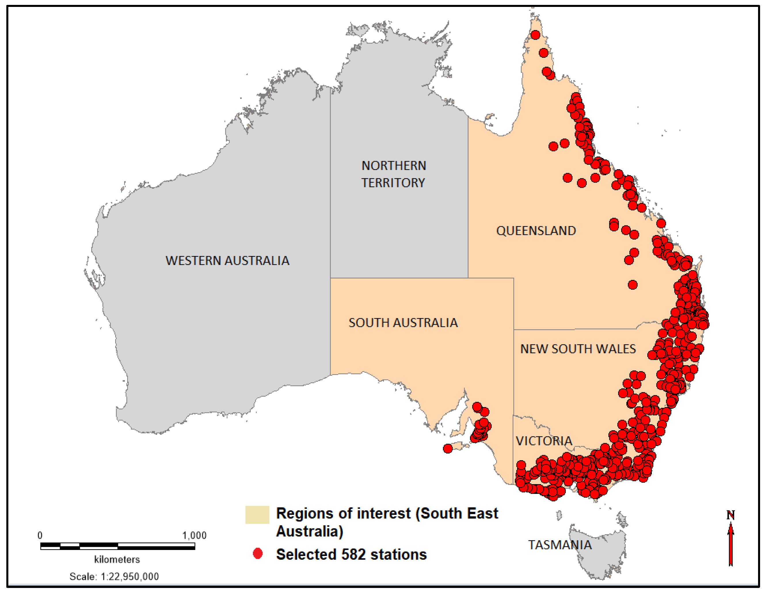
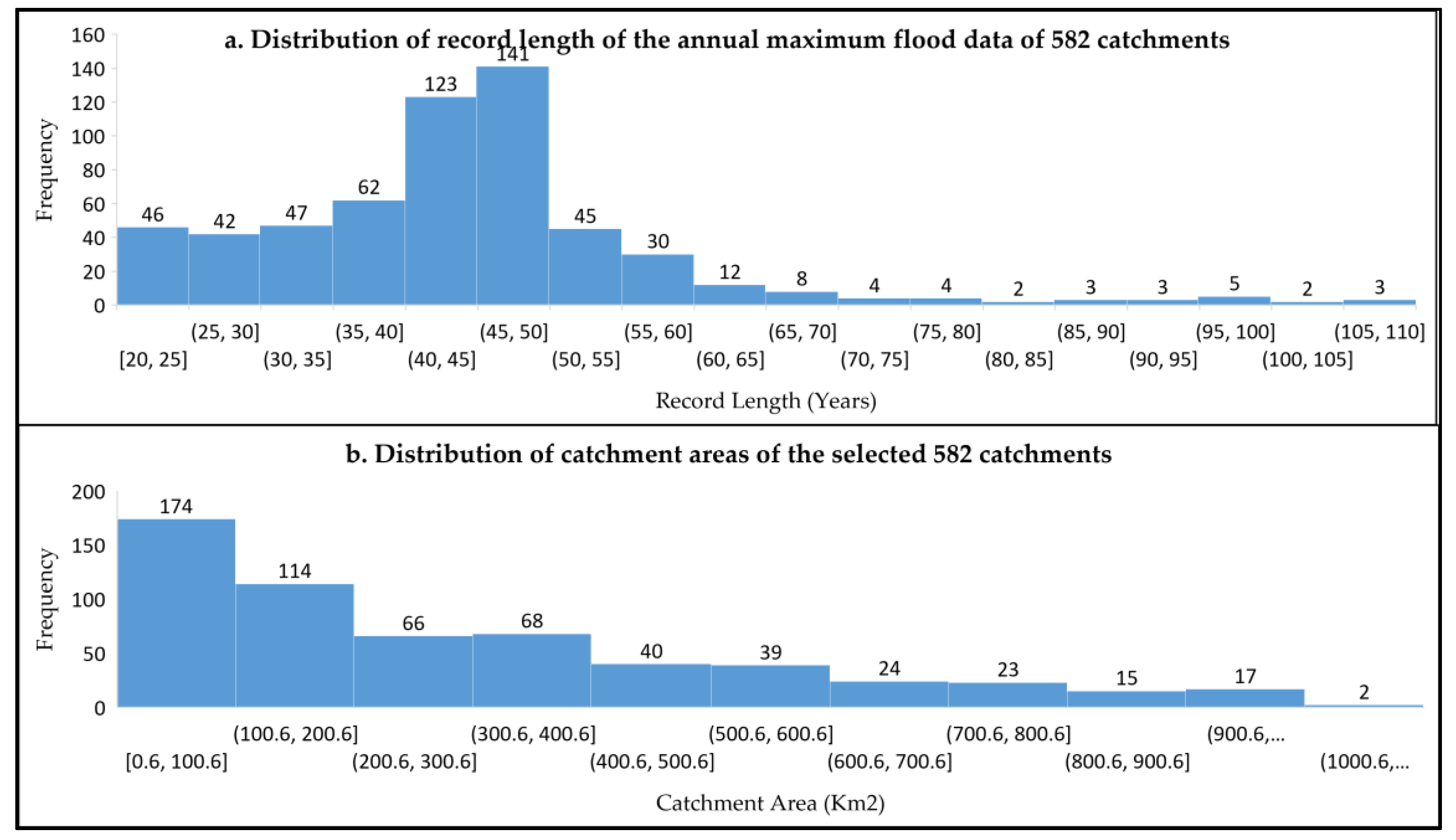
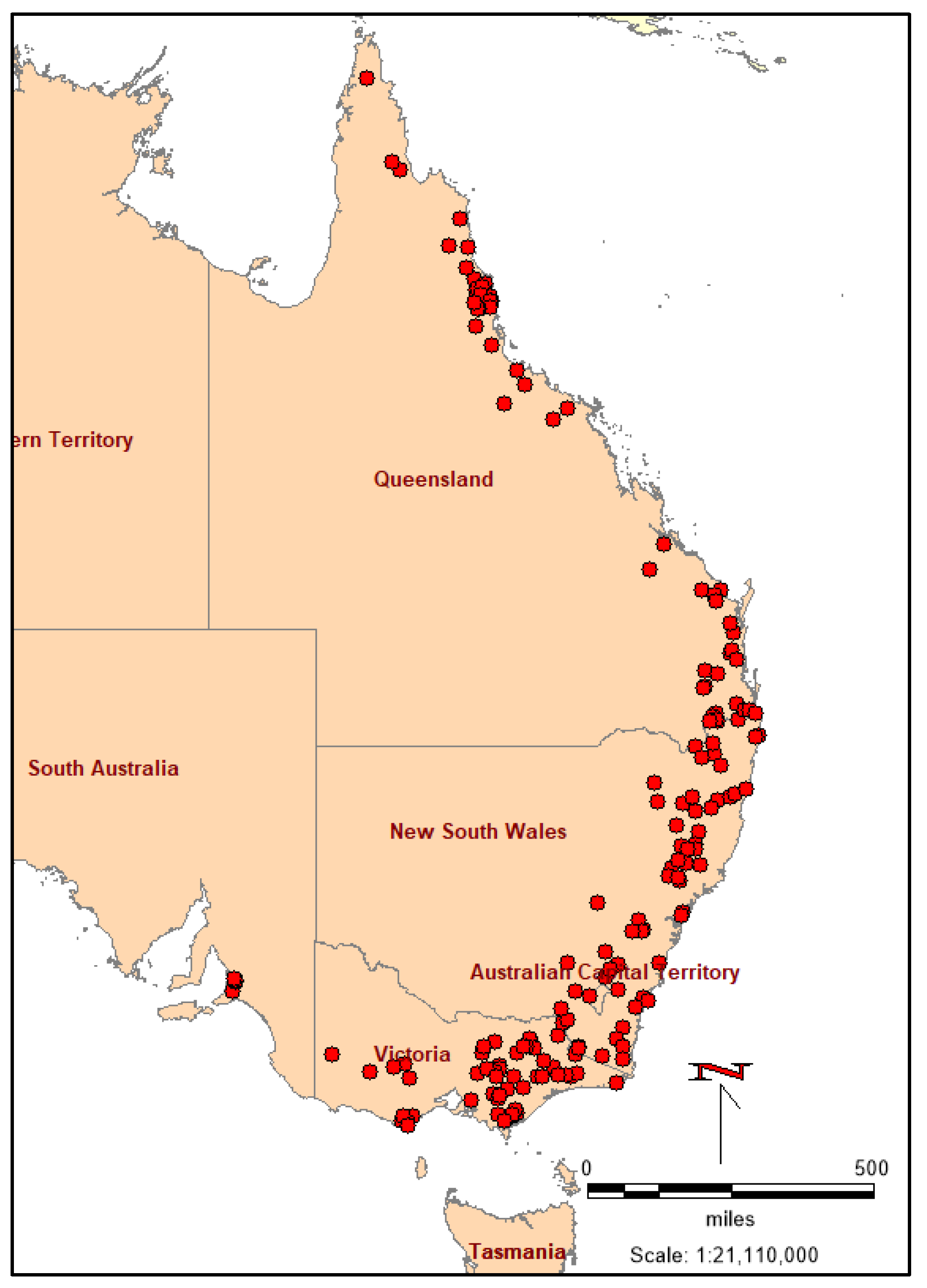
2. Study Area and Data

We selected eastern Australia for this study since it has a high density of gauging stations with long AM flood data. A total of 176 stream gauging stations from New South Wales (NSW), 195 from Queensland (QLD), 183 from Victoria (VIC), and 28 from South Australia (SA) (total 582 stations) were selected. These stations were used in Project 5 of the Australian Rainfall and Runoff (ARR) upgrade project using AM flood data until 2011 [6]; however, we updated the AM flood data until 2018 for these stations as part of this study. Figure 1 illustrates the study region and geographical distribution of the selected stations. Figure 2a depicts the distribution of the AM flood record lengths of the selected 582 stations. The average record length of the AM flood data for the selected 582 stations is 44 years, ranging from 20 to 109 years. Among these stations, 86% have a record length of at least 30 years, and only 13% stations have a record length greater than 55 years. It should be noted that a 20-year record length is too small to carry out meaningful FFA, and, hence, caution should be exercised with the results of the stations (used in this study) having record lengths in the range of 20 to 29 years. Figure 2b depicts the distribution of catchment areas for the selected stations. The selected stations have an average catchment area of 289 km², ranging from 1 km² to 1036 km². Among the stations, 79% are smaller than 500 km² and 21 are larger than 500 km².

3. Methodology

In this study, special consideration is given to the challenges posed by the presence of PILFs in AM flood data. Therefore, the MGB test is selected for its ability to identify multiple PILFs in the AM flood series to overcome the limitation of the original GB test, which can detect only one outlier in a given station’s AM flood series at a time [15].

GEV and LP3 distributions are selected as candidate distributions for FFA because previous studies found that these two distributions are better suited to Australian AM flood data [10]. The estimation of three parameters (location, scale, and shape) of the GEV and LP3 distributions for each of the stations are conducted by L-moments for GEV distribution (due to its robustness and efficiency in estimating distributional parameters) and the Bayesian parameter estimation method for LP3 distribution.

3.1. Log-Pearson Type III Distribution

The LP3 distribution is described by the following equation [27]:

lnQ_T = M + K_TS

(1)

where Q_T is the flood quantile having an annual exceedance probability (AEP) of 1 in T; M is the mean of the natural logarithms of the AM flood series; S is the standard deviation of the natural logarithms of AM flood series; and K_T is frequency factor for the LP3 distribution for AEP of 1 in T, which is a function of the AEP and the skewness of the natural logarithms of the AM flood series [28].

3.2. Generalized Extreme Value Distribution

The GEV distribution is described by the following equation [29]:

$$Q_T=\mu +(\frac{\alpha }{\kappa })[1-{\left(-log\left(\frac{T-1}{T}\right)\right)}^{\kappa }]$$

(2)

where Q_T is the flood quantile having an AEP of 1 in T, µ is the location parameter, α is the scale parameter; and κ is the shape parameter [30]. The at-site FFA for each of the selected stations was conducted using FLIKE software [31]. Flood quantiles were estimated for various AEPs such as 1%, 2%, 5%, 10%, 20%, and 50% (Q₁₀₀, Q₅₀, Q₂₀, Q₁₀, and Q₂, respectively).

3.3. Parameter Estimation Method

In estimating the three parameters (location, scale, and shape) of the GEV and LP3 distributions, L-moments were used for the GEV distribution and Bayesian parameter estimation for the LP3 distribution. The resulting parameters were then used to estimate the selected flood quantiles. Flood quantiles were estimated for various AEPs, and the results were carefully examined to understand the likelihood of extreme events occurring for different return periods at a given station.

3.4. Multiple Grubbs–Beck Test

The GB and MGB test details are given by Cohn et al. [17] and Stedinger [32]. The original GB test, which was recommended in Bulletin 17B [16], describes a low outlier threshold by the following equation:

$$X_{crit}=\widehat{\mu }-K_n\widehat{\sigma }$$

(3)

where K_n is a one-sided, 10% significance-level critical value for an independent sample of n normal variates, and µ and σ are the sample mean and standard deviation of the whole data set [19]. Any observation less than X_crit is labelled as a ‘‘low outlier’’ [17]. Any observation less than X_crit is labelled as a ‘‘low outlier’’ [16,17]. Bulletin 17B [16] uses a conditional probability adjustment to remove low outliers from AM flood data and adjust the frequency curve [16,17]. K_n values are arranged in Section A4 of the Interagency Advisory Committee on Water Data (IACWD) [16] ], based on Table A1 in Grubbs and Beck [13]. Stedinger et al. [32] presents an approximation for 5 ≤ n ≤ 150:

$$K_n\approx -0.9043+3.345\sqrt{lo{g}_{10}\left(n\right)}-0.4046 lo{g}_{10}\left(n\right)$$

(4)

The original GB test can detect one outlier/PILF in the AM flood series of a given station in one go [15]. However, AM flood series may contain more than one low outlier. To overcome this limitation, Rosner [20,21] developed a generalised Extreme Studentised deviate (ESD) to detect one or more outliers from a data set, which is defined as:

$$T_1=\frac{max\left|X_i-\overline{X} \right|}{\widehat{\sigma }}$$

(5)

where $\overline{X}$ and $\widehat{\sigma }$ denote the sample mean and standard deviation of the whole observation [20,21]. The test removes the observation that maximises $\left|X_i-\overline{X} \right|$ and recomputes $T_2$ using the remaining n − 1 data observations [20,21]. Then, it repeats this process until the r number of data points are removed (where r is the number of outliers).

Cohn et al. [17] developed a generalization of the GB test, called the MGB to be able to identify multiple PILFs. In order to consider whether logarithms of AM series {$X_{\left[1:n\right]}, X_{\left[2:n\right]}, \dots ..,X_{\left[k:n\right]}$} are reliable with a normal distribution and the other observations in the sample, Cohn et al. [17] examine a statistic ${\tilde{\omega }}_{\left[k:n\right]}$ which is defined by the following equation:

$${\tilde{\omega }}_{\left[k:n\right]}\equiv \left(X_{\left[k:n\right]}-{\widehat{\mu }}_k\right)/{\widehat{\sigma }}_k$$

(6)

$${\widehat{\mu }}_k\equiv \frac{1}{n-k}{\sum }_{j=k+1}^n{X}_{\left[j:n\right]}$$

(7)

$${{\widehat{\sigma }}^2}_k\equiv \frac{1}{n-k-1}{\sum }_{j=k+1}^n{\left(X_{\left[j:n\right]}-{\widehat{\mu }}_k\right)}^2$$

(8)

where $X_{\left[k:n\right]}$ represents the k_th smallest observation in the flood sample, while ${\widehat{\mu }}_k$ is the partial mean and ${{\sigma }^2}_k$ is the partial variance which are calculated using only the observations greater than $X_{\left[k:n\right]}$ [17].

The Multiple Grubbs-Beck (MGB) test was employed to identify PILFs in the AM flood series. Statistical measures were calculated such as the mean and standard deviation to assess the robustness of the detected outliers.

3.5. Comparison of Results

To further assess the differences between GEV and LP3 distributions (with and without censoring), the absolute percentage difference between the quantiles estimated by the two distributions was calculated using the following equation:

$$\mathrm{Absolute} \mathrm{Percentage} \mathrm{Difference}=\frac{\left|X_1-X_2\right|}{X_1}\times 100$$

(9)

where X₁ represents the flood quantiles from the GEV distribution at a specified AEP and, X₂ represents the flood quantiles from the LP3 distribution (with or without censoring) at the same AEP.

This measure represents the relative variation between the two distributions as a percentage at different AEPs focusing on the effect of censoring low flows in FFA. A higher value indicates a larger difference in the estimated quantiles, while a lower value suggests a closer agreement between the two distributions. The analysis was performed for various AEPs, including 1%, 2%, 5%, 10%, 20%, and 50%, providing a comprehensive understanding of the difference between the GEV and LP3 distributions in representing extreme events in the AM flood series with and without censoring.

3.6. Regression Analysis

A general linear regression model is given by the following equation:

$$Y={\beta }_0+{\beta }_1{X}_1+{\beta }_2{X}_2+{\beta }_3{X}_3+\dots +\epsilon$$

(10)

where Y is is the number of censoring data points (dependent variable); ${\beta }_0$ is the intercept; ${\beta }_1, {\beta }_2, {\beta }_3\dots$ are the regression coefficients for the corresponding catchment characteristics; $X_1, X_2, X_3\dots$ are the catchment characteristic variables; and $\epsilon$ denotes the error term.

T-statistics and p-values are evaluated for a significance level of 0.05. A p-value less than 0.05 indicates a statistically significant association. Multiple R, co-efficient of determination (R²), and adjusted R² are calculated to assess the strengths of the linear relationship.

4. Results and Discussion

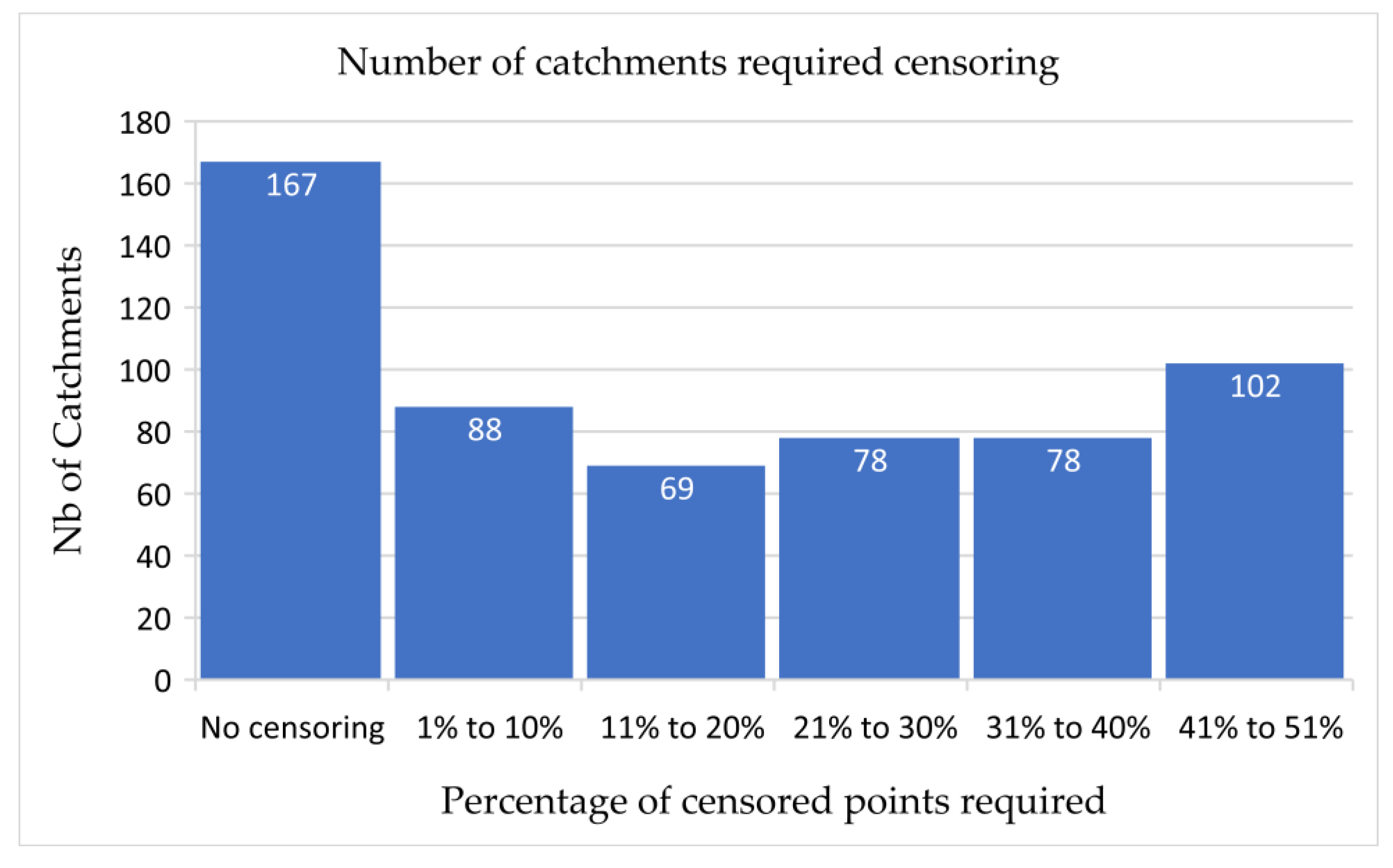
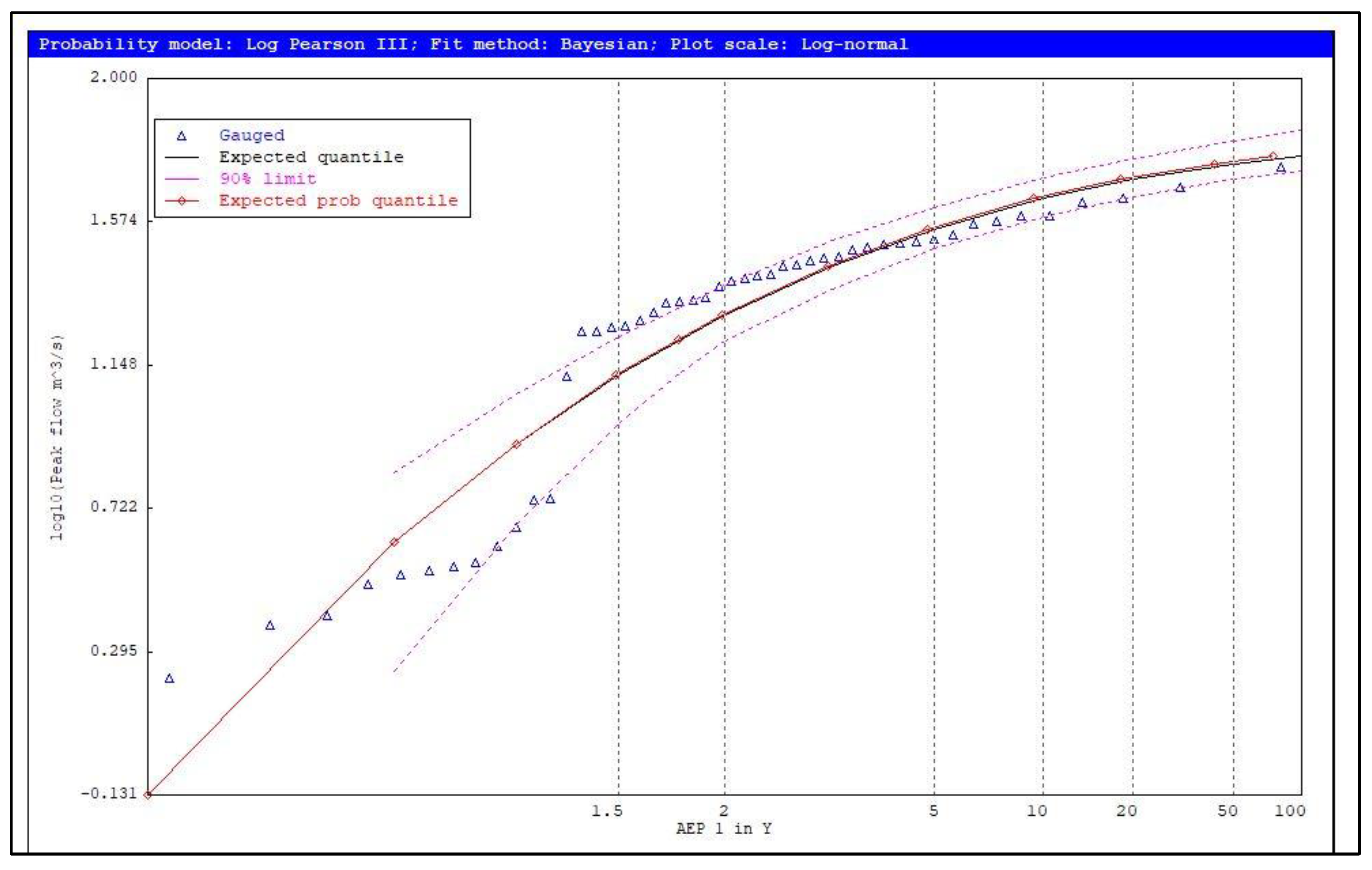
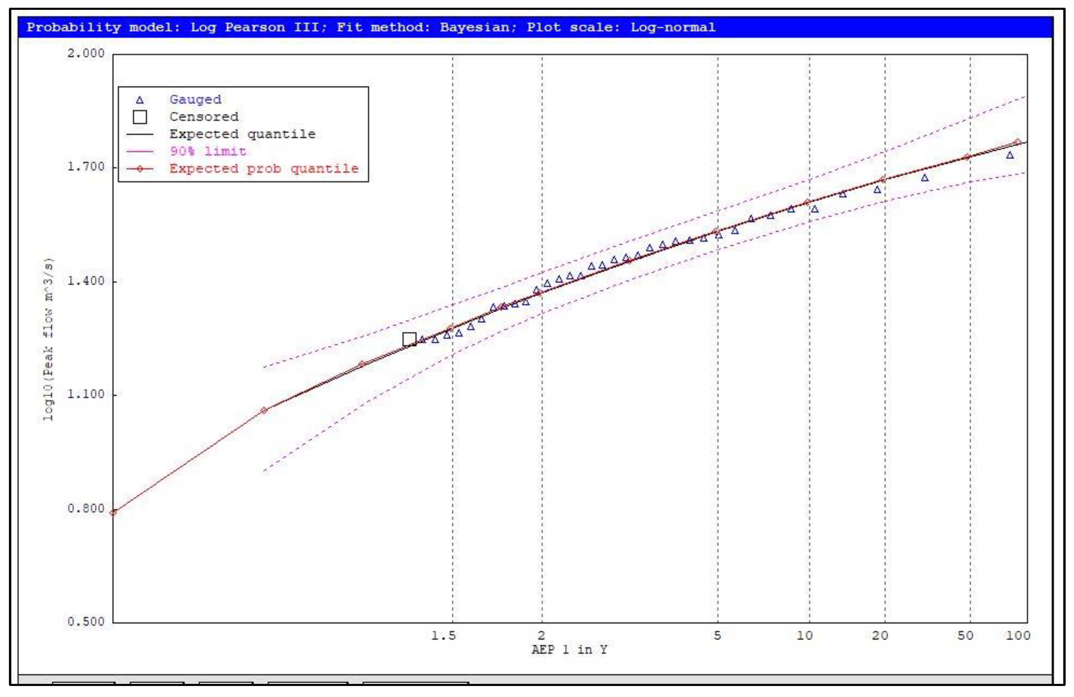
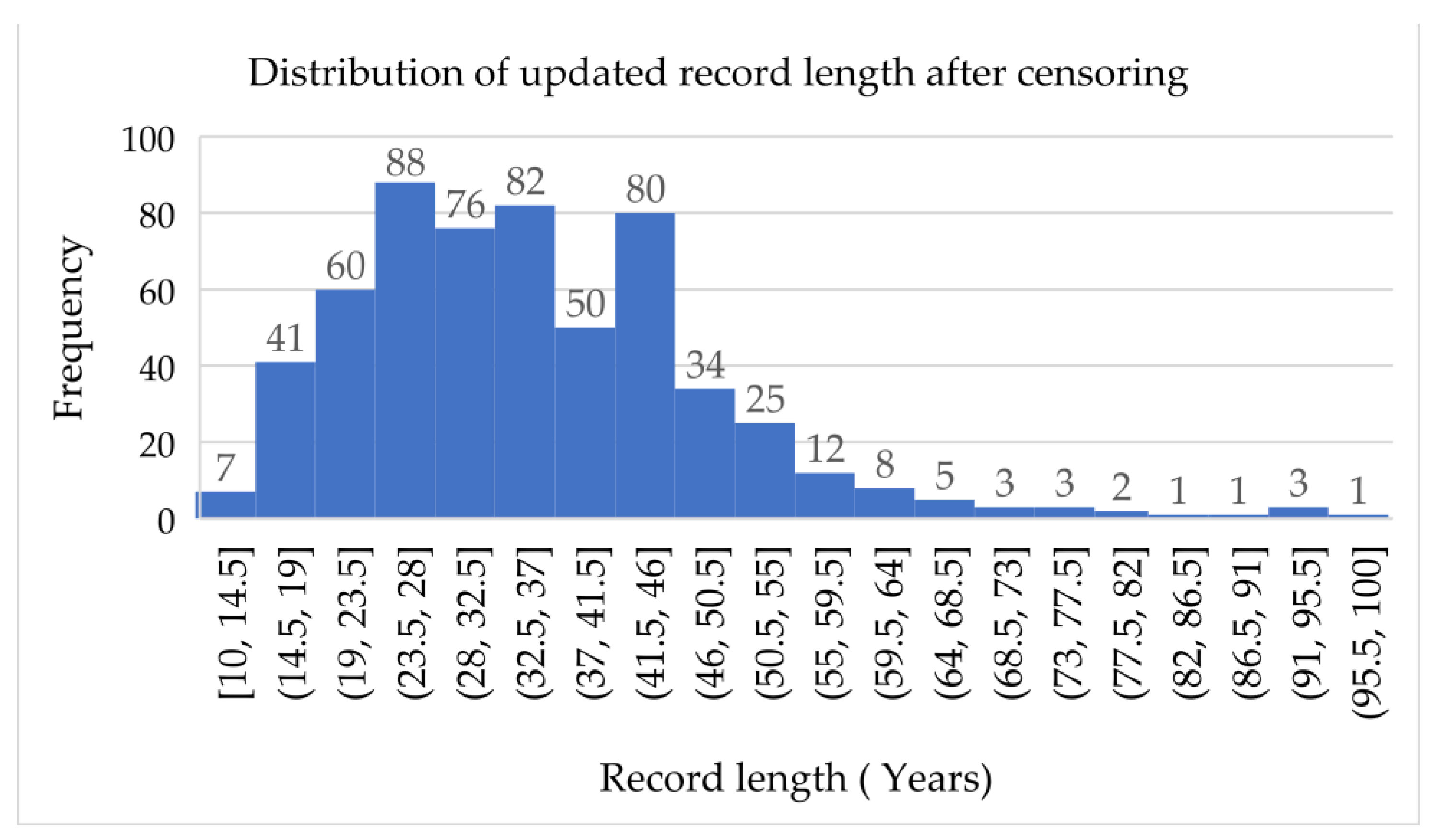
4.1. Identification of Potentially Influential Low Flows (PILFs)

For NSW, it was found that 58 out of 176 stations did not require any censoring and for 30 stations, more than 40% of AM flood data points contain PILFs that needed censoring. For VIC, 51 out of 183 stations did not require any censoring, while 40 stations required censoring for more than 40% of AM flood data points. For SA, it was found that 4 out of 28 stations did not require any censoring, while 5 stations required censoring for more than 40% of AM flood data points. For QLD, 54 out of 195 stations did not require censoring, while 35 stations required censoring for more than 40% of AM flood data points.

Figure 3 shows that 27% (167 out of 582) of stations do not require any censoring; for 88 stations, the MGB test detects between 1 and 10% of the AM flood data points as PILFs; for 69 stations, the MGB test detects between 11% and 20% of AM data points as PILFs. For 78 stations, the MGB test identifies between 21 and 30% of AM data points as PILFs; for 78 stations, the MGB test detects between 31 and 40% of the AM data points as PILFs; and for 102 stations, the MGB test detects at least 41 PILFs. Overall, 71% of the stations contain PILFs. Rahman et al. [22], note that the MGB test detects 40% to 50% of the AM flood series as PILFs at 10 stations in Eastern Australia, which has a temperate climate. Comparing to the USA, Barth et al. [27] report that up to 50% of the peak flows are identified as PILFs using the MGB test in AM flood series from 624 stations in the central and southern coast of California, which is mainly due to precipitation from cold season rainfall. Paretti et al. [32] examine outliers in Arizona (in the Western United States) using the MGB test and identify around 12% of all the AM flood data points as PILFs, which is most likely due to the fact that Arizona is an arid, drought-prone state in the USA.

Figure 4 shows the fitting of GEV distribution to the AM flood data of station 226222 from VIC; Figure 5 shows the LP3 distributions fitting to station 226222 without censoring; and Figure 6 shows the LP3 distribution fitting considering 13 censored data points. The distinction between these three graphs is striking. Thus, fitting the LP3 distribution (with censoring) and GEV distribution (without censoring) is much better than fitting the LP3 distribution without censoring, as the latter shows how far many points are located from the fitted line. The variation in the shape of the graph is obvious, and the results are similar to those reported by Rahman et al. [22], who concluded that the use of the MGB test provides a better fit for the LP3 distribution to the AM flood data series of ten stations in Eastern Australia. Also, Plavsic et al. [33] found that LP3 distribution is very sensitive to the presence of low outliers, and using the MGB test improves the distributional fitting.

Figure 7 shows the location of the 415 stations that require censoring, while Figure 8 shows the percentage of AM flood points that require censoring. The MGB test detects 1.2% to 51.7% of the AM flood data points as PILFs for 415 stations. It can be seen that stations in North-western Victoria require more data points to be censored in fitting the LP3 distribution. Figure 9 depicts the location of the stations that do not require censoring (167 stations). It was discovered that 64 NSW stations, 75 QLD stations, 13 SA stations, and 76 VIC stations have a percentage of censoring points greater than 25% of the total AM records at a station.

Figures S1–S6 (can be seen in the Supplementary Materials) show how the censoring of PILFs affects the fitting of the LP3 distribution to the AM flood data for station 215004 from NSW. It shows the difference in fitting the LP3 distribution by censoring 0, 5, 13, 21, 23, and 31 data points, respectively. The application of the MGB test identifies, in total, 31 PILFs, and the fitting of the LP3 distribution appears to be the best in the last graph (Figure S6) (where all the 31 censored points are applied) compared to the first one (Figure S1) (where there are 0 censored point). Similar to Lamontagne et al. [24], the censoring of PILFs using the MGB test improves the fitting of the LP3 distribution to the AM flood data series at a given station.

After the application of the censoring procedure with the LP3 distribution, Figure 10 displays a new distribution of data lengths (after censoring), which shows that 48 stations have censored data lengths less than 20 years (and 534 stations have a censored data length of 20 years or higher). As a 20-year data length is too small to carry out meaningful FFA, these 48 stations were excluded from further analysis. However, there are 165 stations that have a censored data length in the range of 20 to 29 years. Generally, a 30-year data length is considered to be adequate for a meaningful FFA; hence, caution should be exercised when interpreting the FFA results of these stations (having a data length smaller than 30 years).

Figure 11 shows a boxplot displaying the variations in flood quantiles for 1% AEP using the GEV distribution without censoring and the LP3 distribution with the MGB test and censoring. The plot shows that 50% of the 1% AEP quantiles vary between a minimum of −4% and a maximum of 22% for almost all the states. Furthermore, in NSW, for example, 75% of the variations are less than 55% and 50% are greater than 8% (median value). Regarding the upper and lower whisker values, it is found that the variation of flood quantiles for the 1% AEP flood quantiles falls in the range of −45% to 72% in QLD, −42% to 79% in VIC, −60% to 84% in NSW, and −18% to 30% in SA. However, except for a small number of stations, there is no significant difference in the 1% AEP flood quantiles between the GEV and LP3 distributions. These findings support the results of Rahman et al. [22], who demonstrated that in most of their 10 study stations, the GEV distribution and LP3 distribution (with censoring) produce very similar results.

Table 2. Variation between the absolute values of flood quantiles for 1% AEP for the stations that required censoring.

Distribution	Percentage of Absolute Variation for Q100
	QLD				VIC
	Min	Max	Mean	St. Dev.	Min	Max	Mean	St. Dev.
GEV—LP3 with censoring	0.29	46.57	11.45	8.57	1.10	41.62	12.46	10.24
GEV-LP3 (no censoring)	0.60	69.48	10.47	12.77	0.10	321.69	16.59	42.25
LP3 (censoring)—LP3 (no censoring)	0.32	57.18	12.32	11.74	0.63	291.43	18.68	38.16
Distribution	Percentage of Absolute Variation of Q100
	NSW				SA
	Min	Max	Mean	St. Dev.	Min	Max	Mean	St. Dev.
GEV—LP3 with censoring	0.01	37.60	12.67	7.38	0.15	30.03	11.77	8.50
GEV-LP3 (no censoring)	0.35	55.91	10.83	12.81	0.10	27.93	9.73	8.55
LP3(censoring)—LP3 (no censoring)	0.40	72.79	14.13	14.21	0.48	53.66	16.18	15.88

shows the variation between the absolute values of the flood quantiles for 1% AEP estimated by different distributions for QLD, VIC, NSW and SA. It is found that the variation of the absolute values of the flood quantiles for 1% AEP gets bigger if there is no censoring.

Figure 12 depicts the percentage of the variation in flood quantiles (Q10, Q20, Q50, and Q100) estimated using two methods: LP3 with censoring and GEV without censoring. As shown, the variation for Q10 ranges between −2.91% and 51.09%, and for eight stations, the quantiles estimated by GEV were greater than the quantiles estimated by LP3. The variation for Q20 ranges between −7.29% and 60.71%, and for 12 stations, the quantiles estimated by GEV were greater than the quantiles estimated by LP3 distribution. The variation for Q50 ranges between −30.21% and 77.79%, and for 103 stations, the quantiles estimated by the GEV distribution were greater than the quantiles estimated by the LP3 distribution. The variation for Q100 ranges between −59.79% and 87.21%, and for 178 stations, the quantiles estimated by GEV were greater than the quantiles estimated by LP3. It was also demonstrated that the number of stations with a negative difference in GEV distribution increases with 10%, 5%, 2%, and 1% AEPs, respectively. Interestingly, the stations showed a positive difference in flood quantiles by the GEV, which decreases with AEPs of 10%, 5%, 2%, and 1%. Compared to Rahman et al. (2014), the variations of the flood quantiles Q100 for 10 stations in Eastern Australia, estimated by two methods, LP3 with the MGB test and GEV with L-moments, range between −18.19% and 38.01%. Figure 12 shows that the variations of the flood quantiles Q100 for 87% of the stations (465/534) fall within this range. As a result, these findings highlight the similarity in the results in flood quantile estimates between the LP3 and GEV distributions.

Figure 13 depicts the absolute variation of flood quantiles for various AEPs ranging from Q1 to Q10000 between GEV with L-moments and LP3, with and without censoring. The comparison was performed on the stations that required censoring. As shown, the quantile variations are larger when there is no censoring. Thus, censoring improves the fitting of the LP3 distribution. Also, censoring enhances accuracy of flood quantiles, particularly at higher AEPs.

4.2. Relationship between Number of Censored Data Points and Catchment Characteristics

Regression analysis was conducted to investigate the relationship between the number of censoring data points in the AM flood series and catchment characteristics such as base-flow index (BFI) (volume factor and peak factor), mean annual rainfall (MAR), and the catchment shape factor (SF). For this, only South Australian (SA) stations are used. For the 28 SA stations, the catchment characteristics data were obtained from the ARR data hub. The regression results in

Table 3. Linear regression outputs exhibiting relationship between censored points and catchment characteristics.

Regression Statistics			Coefficients	Standard Error	t Stat	p-Value
Multiple R	0.66	Intercept	9.64	8.281	1.164	0.256
R2	0.43	BFI (volume factor)	−12.04	9.439	−1.28	0.215
Adjusted R2	0.33	BFI (peak factor)	29.917	21.478	1.393	0.177
Standard error	6.2	(MAR) (mm)	−0.016	0.007	−2.31	0.03
Observations	28	SF	12.822	5.599	2.29	0.032

revealed that the MAR and SF are statistically significant, with p-values less than 0.05, indicating a possible association with the number of censoring data points. The volume and peak baseflow factors, on the other hand, did not exhibit statistical significance, as their p-values exceeded the 5% significance level. The correlation coefficient (multiple R) of 66% suggested a reasonable linear relationship (Table 3). Nevertheless, the coefficient of determination (R²), representing the goodness of fit, indicated a modest overall fit of 43%. This implies that the examined catchment characteristics explain only a limited portion of the variability in the number of censored points in the AM flood series in Eastern Australia. While the initial hypothesis focused on catchment characteristics, the results indicate a weak correlation, and, hence, we acknowledge the importance of exploring alternative hypotheses to better understand the origin of censored data in the AM flood series. It is crucial to discover other potential factors contributing to the presence of censored data. Future investigations should consider larger datasets and additional catchment characteristics, including those from other states, to provide a more comprehensive understanding of this phenomenon.

5. Conclusions

This study focused on the treatment of low-flow outliers in flood frequency analysis (FFA). We employed log-Pearson type 3 (LP3) and generalized extreme value (GEV) distributions to carry out FFA using FLIKE software. Of the 582 stations, 71% required low-flow censoring when applying the LP3 distribution in FFA. This study shows that the multiple Grubbs and Beck (MGB) test is quite effective in Australia to identify low-flow outliers in annual maximum (AM) flood data. In many cases, about one third of AM flood data points at a given station need censoring to fit the LP3 distribution. North-western Victoria required more censoring than other parts of Australia. This part of the study area is drier compared to the other parts, which means that there are many low AM flow data points in the AM flood series due to frequent droughts. In cases using the GEV distribution with L-moments, censoring may not be needed, as the L-moments method is less affected by the presence of outliers compared to ordinary product moments. Censoring is generally needed for the LP3 and log-normal distributions, since these two distributions require the log-transformation of AM flood data series before fitting a distribution. It should be noted that log-transformation provides higher weight to data points representing smaller peak discharges in the AM flood series. The record length of a station after censoring should not be too small to ensure that the FFA results are not much affected by sampling errors. However, censoring does not mean discarding the low-flow outliers in fitting a probability distribution to AM flood data. The impact of censoring was more pronounced for smaller return periods than larger ones, as expected. For South Australia, the number of censored low-flow data points in the AM flood series was found to have a modest correlation with catchment characteristics (base-flow index, mean annual rainfall, and catchment shape factor). Given the fact that the correlation was modest, additional research is needed to confirm this finding using data from all Australian states and including additional catchment characteristics that could affect censoring. The findings of this study may be useful to update the FFA methods recommended in Australian Rainfall and Runoff (national guide) [34].

References

1. Stefanidis, S.; Stathis, D. Assessment of flood hazard based on natural and anthropogenic factors using analytic hierarchy process (AHP). Nat. Hazards 2013, 68, 569–585. [Google Scholar] [CrossRef]
2. Insurance Council of Australia (ICA). Updated Data Shows 2022 Flood Was Australia’s Costliest. Available online: https://insurancecouncil.com.au/wp-content/uploads/2022/05/220503-East-Coast-flood-event-costs-update.pdf (accessed on 3 May 2022).
3. Ahmad, I.; Waqas, M.; Almanjahie, I.M.; Saghir, A.; Haq, E.U. Regional flood frequency analysis using linear moments and partial linear moments: A case study. Appl. Ecol. Environ. Res. 2019, 17, 3819–3836. [Google Scholar] [CrossRef]
4. Ekeu-Wei, I.T.; Blackburn, G.A.; Giovannettone, J. Accounting for the Effects of Climate Variability in Regional Flood Frequency Estimates in Western Nigeria. J. Water Resour. Prot. 2020, 12, 690. [Google Scholar] [CrossRef]
5. Garmdareh, E.S.; Vafakhah, M.; Eslamian, S.S. Regional flood frequency analysis using support vector regression in arid and semi-arid regions of Iran. Hydrol. Sci. J. 2018, 63, 426–440. [Google Scholar] [CrossRef]
6. Haddad, K.; Rahman, A.; Weinmann, P.E.; Kuczera, G.; Ball, J. Streamflow data preparation for regional flood frequency analysis: Lessons from southeast Australia. Australas. J. Water Resour. 2010, 14, 17–32. [Google Scholar] [CrossRef]
7. Requena, A.I.; Ouarda, T.B.; Chebana, F. Flood frequency analysis at ungauged sites based on regionally estimated streamflows. J. Hydrometeorol. 2017, 18, 2521–2539. [Google Scholar] [CrossRef]
8. Desai, S.; Ouarda, T.B. Regional hydrological frequency analysis at ungauged sites with random forest regression. J. Hydrol. 2021, 594, 125861. [Google Scholar] [CrossRef]
9. Kousar, S.; Khan, A.R.; Ul Hassan, M.; Noreen, Z.; Bhatti, S.H. Some best-fit probability distributions for at-site flood frequency analysis of the Ume River. J. Flood Risk Manag. 2020, 13, e12640. [Google Scholar] [CrossRef]
10. Rahman, A.S.; Rahman, A.; Zaman, M.A.; Haddad, K.; Ahsan, A.; Imteaz, M. A study on selection of probability distributions for at-site flood frequency analysis in Australia. Nat. Hazards 2013, 69, 1803–1813. [Google Scholar] [CrossRef]
11. Ahn, K.H.; Palmer, R. Regional flood frequency analysis using spatial proximity and basin characteristics: Quantile regression vs. parameter regression technique. J. Hydrol. 2016, 540, 515–526. [Google Scholar] [CrossRef]
12. Stojković, M.; Prohaska, S.; Zlatanović, N. Estimation of flood frequencies from data sets with outliers using mixed distribution functions. J. Appl. Stat. 2017, 44, 2017–2035. [Google Scholar] [CrossRef]
13. Grubbs, F.E.; Beck, G. Extension of sample sizes and percentage points for significance tests of outlying observations. Technometrics 1972, 14, 847–854. [Google Scholar] [CrossRef]
14. Barnett, V.; Lewis, T. Outliers in Statistical Data; John Wiley and Sons: New York, NY, USA, 1994. [Google Scholar]
15. Grubbs, F.E. Procedures for detecting outlying observations in samples. Technometrics 1969, 11, 1–21. [Google Scholar] [CrossRef]
16. Interagency Advisory Committee on Water Data (IAWCD). Guidelines for Determining Flood Flow Frequency: Bulletin 17-B; Technical Report; Interagency Advisory Committee on Water Data (IAWCD): Washington, DC, USA, 1982; 28p. [Google Scholar]
17. Cohn, T.A.; England, J.F.; Berenbrock, C.E.; Mason, R.R.; Stedinger, J.R.; Lamontagne, J.R. A generalized Grubbs-Beck test statistic for detecting multiple potentially influential low outliers in flood series. Water Resour. Res. 2013, 49, 5047–5058. [Google Scholar] [CrossRef]
18. Interagency Advisory Committee on Water Data (IAWCD). Robust National Flood Frequency Guidelines: What Is an Outlier? Bulletin 17C; IAWCD: Washington, DC, USA, 2013. [Google Scholar]
19. England, J.F., Jr.; Cohn, T.A. Bulletin 17B flood frequency revisions: Practical software and test comparison results. In Proceedings of the World Environmental and Water Resources Congress 2008: Ahupua’A, Honolulu, HI, USA, 12–16 May 2008; pp. 1–11. [Google Scholar]
20. Rosner, B. On the detection of many outliers. Technometrics 1975, 17, 221–227. [Google Scholar] [CrossRef]
21. Rosner, B. Percentage points for a generalized ESD many-outlier procedure. Technometrics 1983, 25, 165–172. [Google Scholar] [CrossRef]
22. Rahman, A.S.; Haddad, K.; Rahman, A. Impacts of outliers in flood frequency analysis: A case study for Eastern Australia. J. Hydrol. Environ. Res. 2014, 2, 17–30. [Google Scholar]
23. Blagojević, B.; Mihailović, V.; Plavšić, J. Outlier treatment in the flood flow statistical analysis. In Međunarodna konferencija Savremena dostignuća u građevinarstvu 25; Građevinski Fakultet: Subotica, Serbia, 2014; Volume 30, pp. 603–609. [Google Scholar]
24. Lamontagne, J.R.; Stedinger, J.R.; Yu, X.; Whealton, C.A.; Xu, Z. Robust flood frequency analysis: Performance of EMA with multiple Grubbs-Beck outlier tests. Water Resour. Res. 2016, 52, 3068–3084. [Google Scholar] [CrossRef]
25. Jaiswal, R.K.; Nayak, T.R.; Lohani, A.K.; Galkate, R.V. Regional flood frequency modeling for a large basin in India. Nat. Hazards 2021, 111, 1845–1861. [Google Scholar] [CrossRef]
26. Mitchell, J.N.; Wagner, D.M.; Veilleux, A.G. Magnitude and Frequency of Floods on Kaua‘i, O‘ahu, Moloka‘i, Maui, and Hawai‘i, State of Hawai‘i, Based on Data through Water Year 2020 (No. 2023-5014); US Geological Survey: Reston, VA, USA, 2023. [Google Scholar]
27. Stedinger, J.R. Frequency analysis of extreme events. In Handbook of Hydrology; McGraw Hill: New York, NY, USA, 1993. [Google Scholar]
28. Chow, V.T. A general formula for hydrologic frequency analysis. Eos Trans. Am. Geophys. Union 1951, 32, 231–237. [Google Scholar]
29. Barth, N.A.; Villarini, G.; Nayak, M.A.; White, K. Mixed populations and annual flood frequency estimates in the western United States: The role of atmospheric rivers. Water Resour. Res. 2017, 53, 257–269. [Google Scholar] [CrossRef]
30. Hosking, J.R. L-moments: Analysis and estimation of distributions using linear combinations of order statistics. J. R. Stat. Soc. Ser. B Methodol. 1990, 52, 105–124. [Google Scholar] [CrossRef]
31. Kuczera, G.; Franks, S. At-Site Flood Frequency Analysis. Australian Rainfall and Runoff: A Guide to Flood Estimation; Geoscience Australia: Canberra, Australia, 2016; pp. 5–99. [Google Scholar]
32. Paretti, N.V.; Kennedy, J.R.; Cohn, T.A. Evaluation of the Expected Moments Algorithm and a Multiple Low-Outlier Test for Flood Frequency Analysis at Streamgaging Stations in Arizona (No. 2014-5026); US Geological Survey: Reston, VA, USA, 2014. [Google Scholar]
33. Plavšić, J.; Mihailović, V.; Blagojević, B. Assessment of methods for outlier detection and treatment in flood frequency analysis. In Proceedings of the Mediterranean Meeting on Monitoring, Modelling and Early Warning of Extreme Events Triggered by Heavy Rainfalls, PON 01_01503-MED-FRIEND Project University of Calabria, Cosenza, Italy, 26–28 June 2014; pp. 181–192. [Google Scholar]
34. Rahman, A.; Haddad, K.; Kuczera, G.; Weinmann, E. Regional flood methods. In Australian Rainfall and Runoff: A Guide to Flood Estimation; Book 3, Peak Flow Estimation; Geoscience, Commonwealth of Australia: Canberra, Australia, 2019; pp. 105–146. [Google Scholar]
Figure 1. Geographical distribution of the selected 582 stream gauging stations in eastern Australia.
Water 16 00535 g001
Figure 2. Distribution of record length of the AM flood data and catchment areas of the selected 582 stations.
Water 16 00535 g002
Figure 3. Number of stations required censoring in this study from 582 stations.
Water 16 00535 g003
Figure 4. Fitting of GEV distribution to station 226222 with L-moments.
Water 16 00535 g004
Figure 5. Fitting of LP3 distribution to station 226222 without censoring.
Water 16 00535 g005
Figure 6. Fitting of LP3 distribution to station 226222 after censoring 13 PILFs.
Water 16 00535 g006
Figure 7. Location of stations that required censoring with LP3 distribution (415 stations).
Water 16 00535 g007
Figure 8. Percentage of AM flood data points that needed censoring.
Water 16 00535 g008
Figure 9. Location of annual maxima (AM) flood data stations that do not need censoring (167 stations).
Water 16 00535 g009
Figure 10. Distribution of new record length of the AM flood data after censoring.
Water 16 00535 g010
Figure 11. Variations in flood quantiles Q100 (1% AEP) between GEV and LP3 distributions with censoring (total: 534 stations; QLD: 186 stations; VIC: 169 stations; NSW: 152 stations; and SA: 27 stations).
Water 16 00535 g011
Figure 12. Percentage variation between flood quantiles (Q10, Q20, Q50, and Q100) estimated by two methods: LP3 with censoring and GEV with L-moments (without censoring) for 534 stations.
Water 16 00535 g012
Figure 13. Absolute variation (%) in flood quantile estimates between GEV and LP3 distributions (with and without censoring) for the stations that required censoring.
Water 16 00535 g013