
Energy Transition in Urban Water Infrastructures towards Sustainable Cities

 ,
,  ,
, 
 ,
,  ,
,  ,
,  , and
, and 
Abstract
1. Introduction
2. Materials and Methods
2.1. Hydraulic Model Simulator
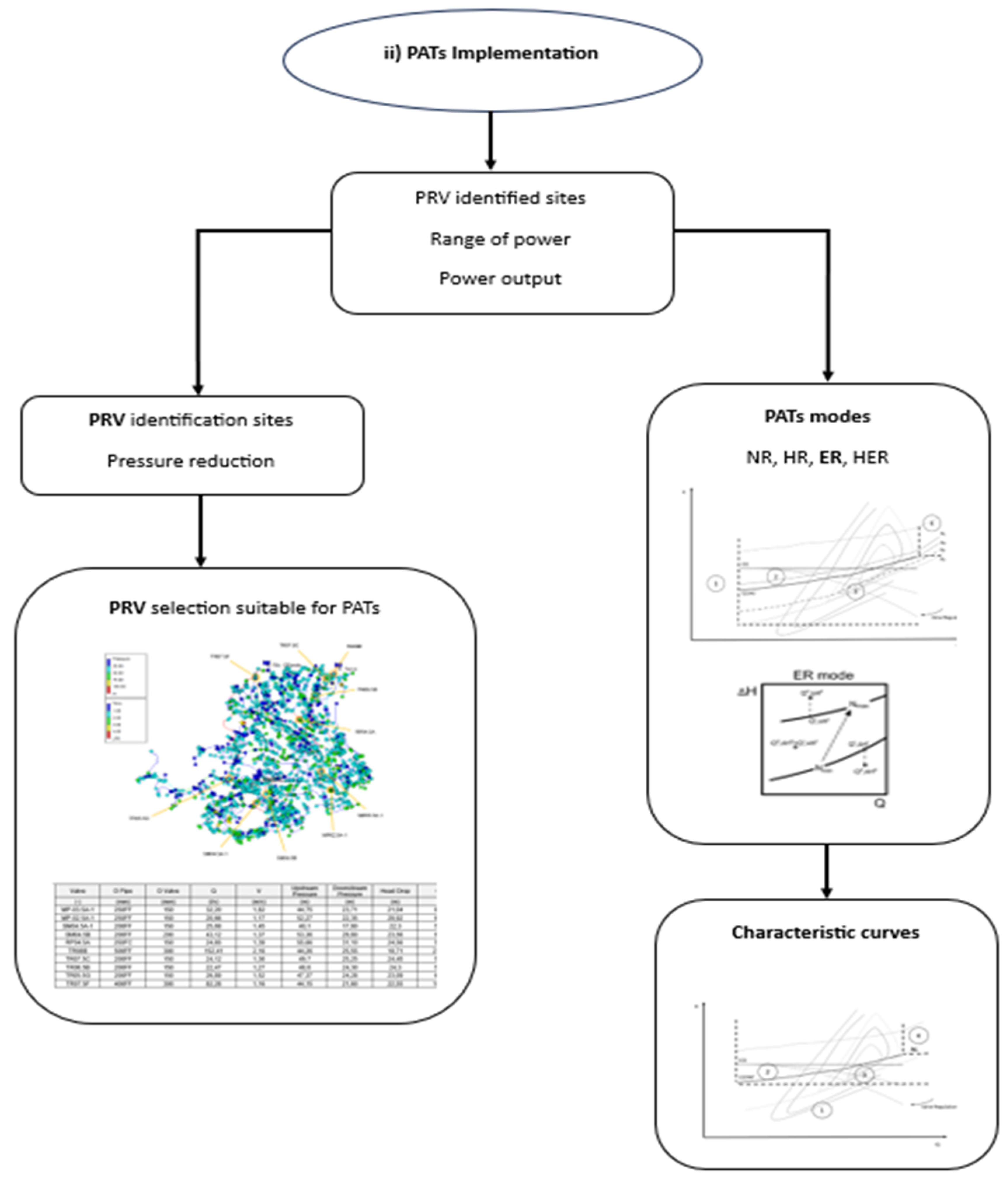
2.2. Energy Recovery with PATs
- Region 1—: ;
- Region 2— or and : ;
- Region 3— and : .
- Region 1— or : ;
- Region 2— and : ;
- Region 3— and : ;
- Region 4— and : .
- Region 1— or : ;
- Region 2— and : ;
- Region 3— and : ;
- Region 4— and : .
2.3. Energy Simulator
2.4. Energy Production
- = power output during standard test conditions in kW.
- = derating factor of solar PV.
- = incident solar irradiance in kW/.
- = incident solar irradiance at Standard test conditions, which is 1 kW/.
- = temperature co-efficient of power.
- = cell temperature of solar PV in °C.
- = cell temperature under standard test conditions, which is 25 °C.
- = wind speed at the hub height of the wind turbine in m/s.
- = wind speed at the anemometer height in m/s.
- = hub height of the wind turbine in m.
- = the surface roughness length in m.
- = anemometer height in m.
- = output power of wind turbine in kW.
- = output power of wind turbine at standard temperature and pressure in kW.
- = actual air density in kg/.
- = air density at STP, which is 1.225 kg/.
- = hydro turbine power output in kW.
- = efficiency of hydro turbine in %.
- = water density, which is 1000 kg/.
- g = acceleration due to gravity 9.81 m/.
- = effective head in m.
- = hydro turbine flow rate in .
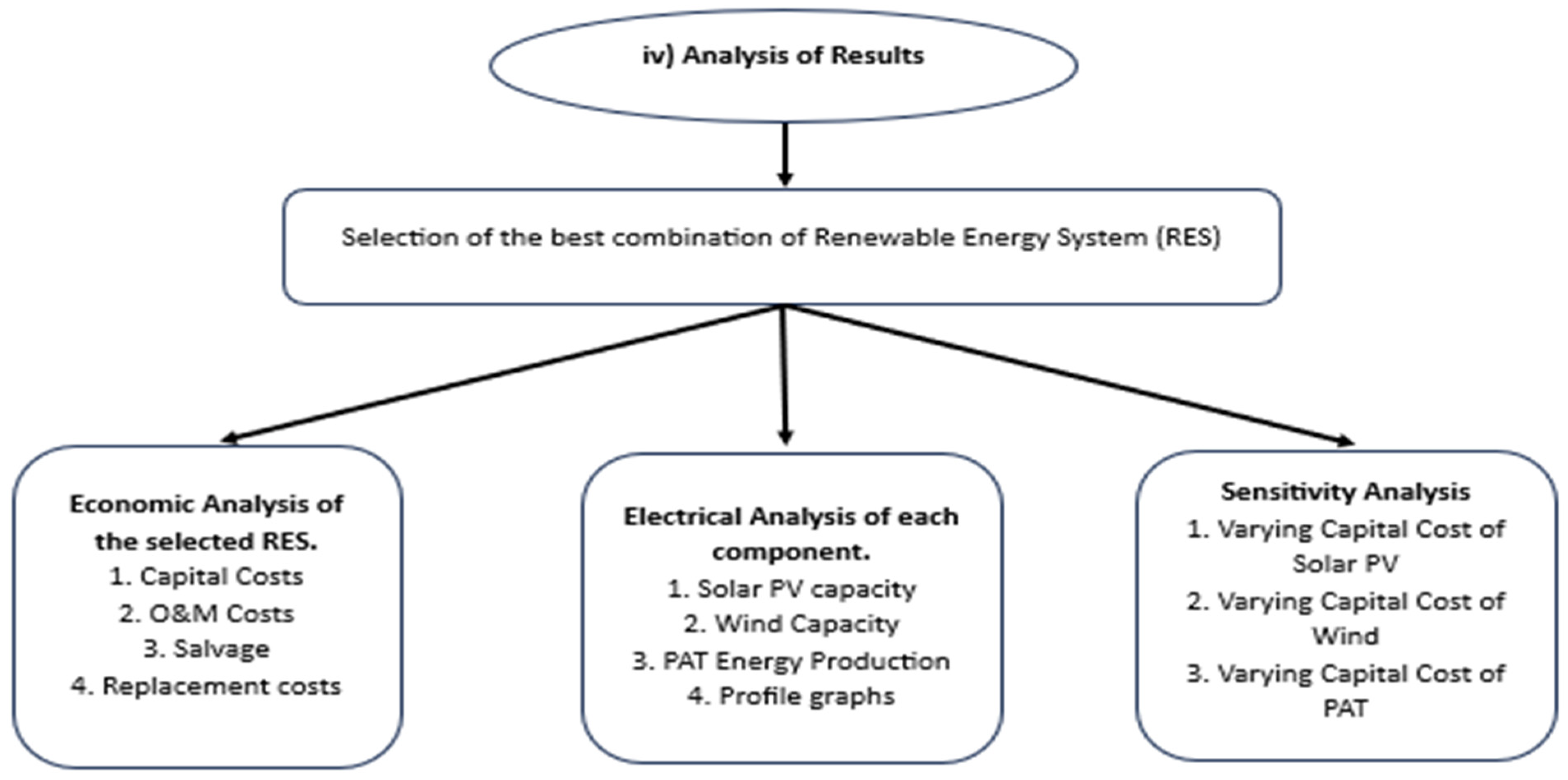
2.5. Methodology for the Analysis of Results
- = total annualized cost of the system in EUR/year.
- = total electrical energy served in kWh/year.
- i = real discount rate.
- = nominal discount rate.
- f = expected inflation rate.
- = discount factor.
- i = real discount rate.
- N = number of years.
3. Results and Discussion
3.1. Brief system Definition
- Establishment of district metered areas (DMAs): This means creating defined zones within the distribution system to facilitate the metering and regulation of pressure levels and flow rates in each area. In the first phase, the primary areas of influence are delineated.
- Effective pressure management: This step focuses on properly regulating pressure to avoid excessive water loss and ensure adequate water supply to consumers.
- Active damage control: In this phase, measures are taken to detect and repair leaks in the system in good time.
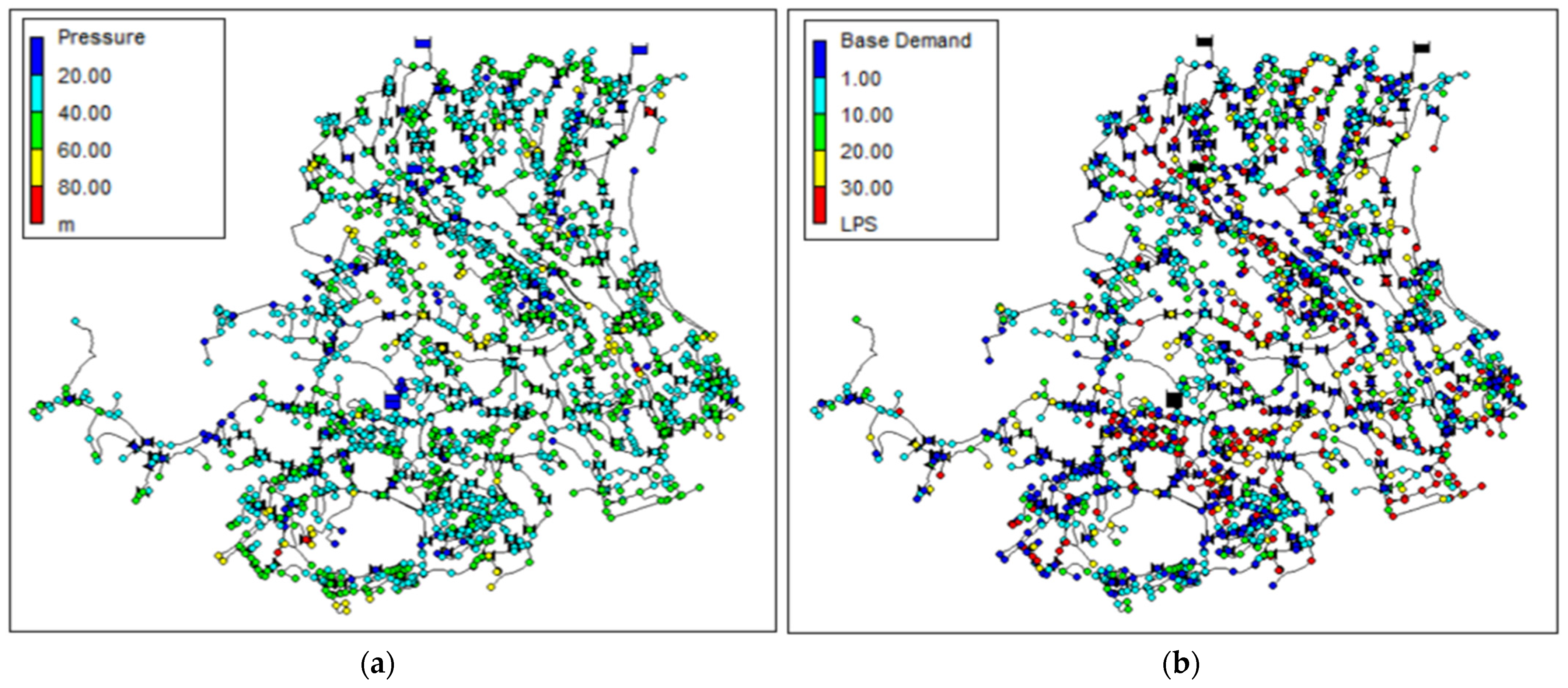
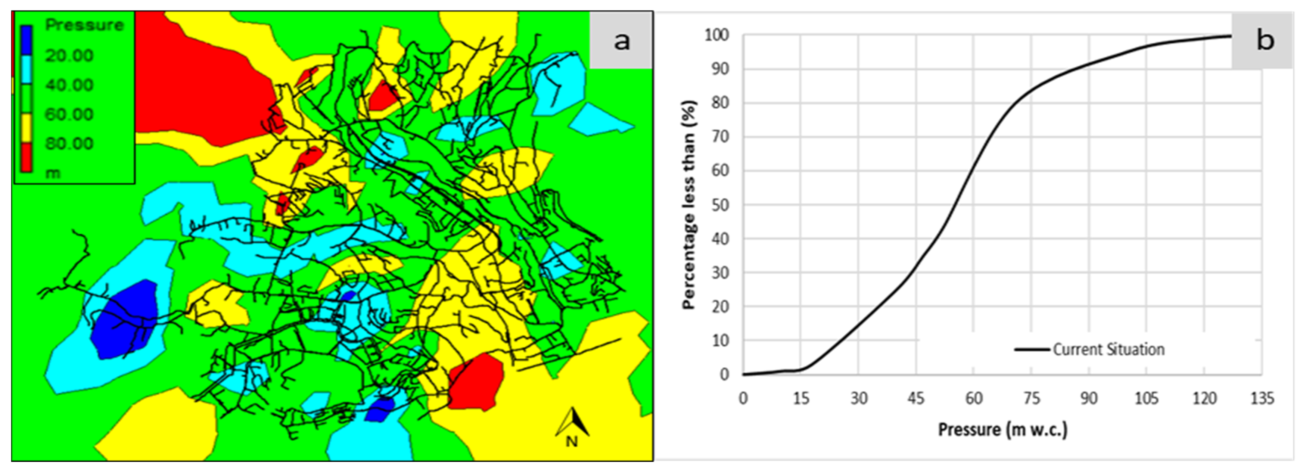
3.2. Hydraulic Simulations
3.2.1. Hydraulic Scenarios
- (i)
- The pressure values of the network decreased to an average value of about 37 m w.c., which is a decrease of 16 m w.c. compared to the previous scenario.
- (ii)
- Only 4% of the nodes in the network registered a minimum pressure above the legal maximum of 60 m w.c.—a significant decrease (35%) from the previous scenario. Moreover, this figure increased slightly to 5% when studied under static boundary conditions, in stark contrast to the 50% recorded in the existing scenario.
- (iii)
- It is particularly noteworthy that most of the network is no longer under excessive pressure, with an average reduction of about 1.6 bar compared to the current situation.
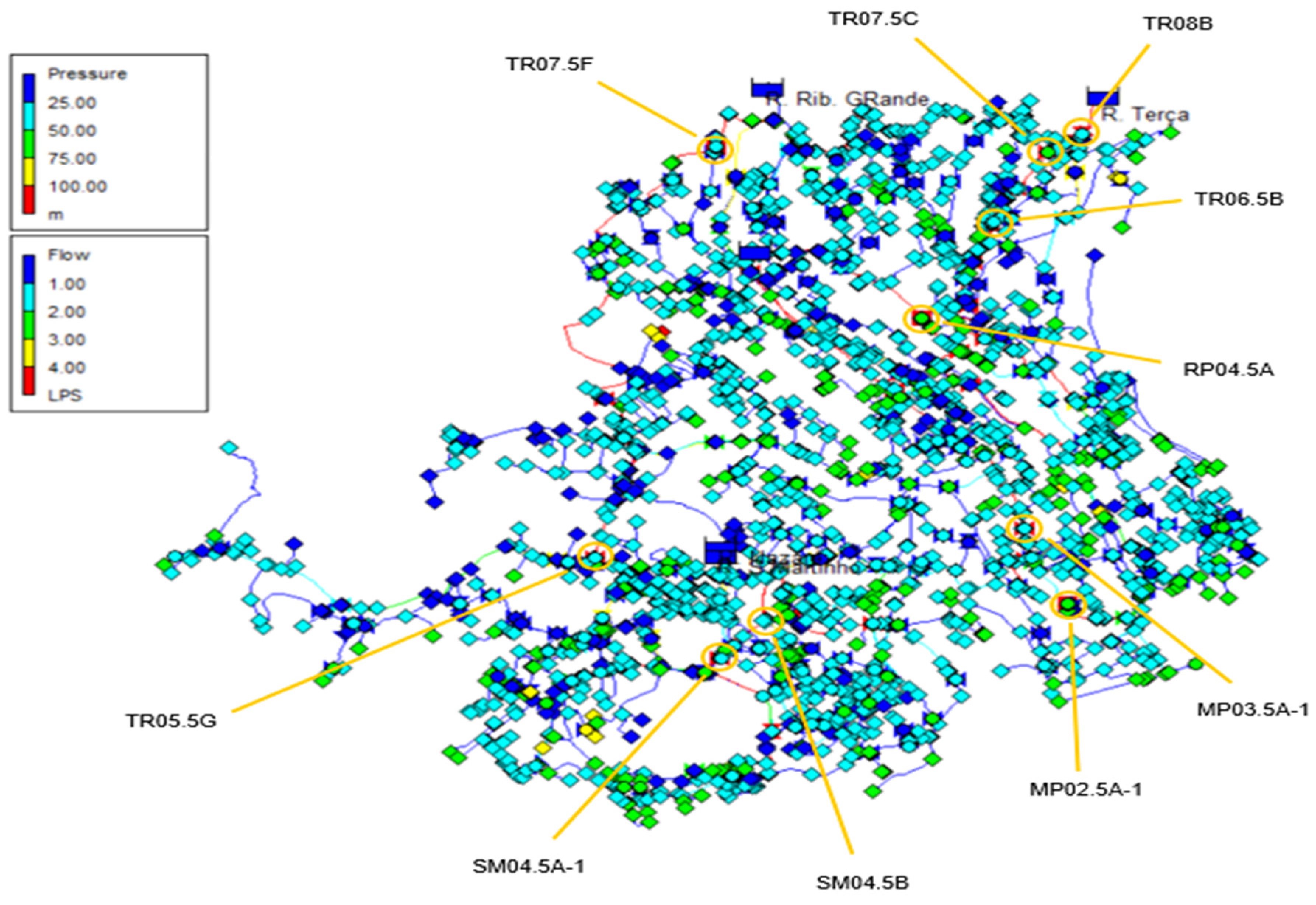
3.2.2. PRV and PAT Characteristics
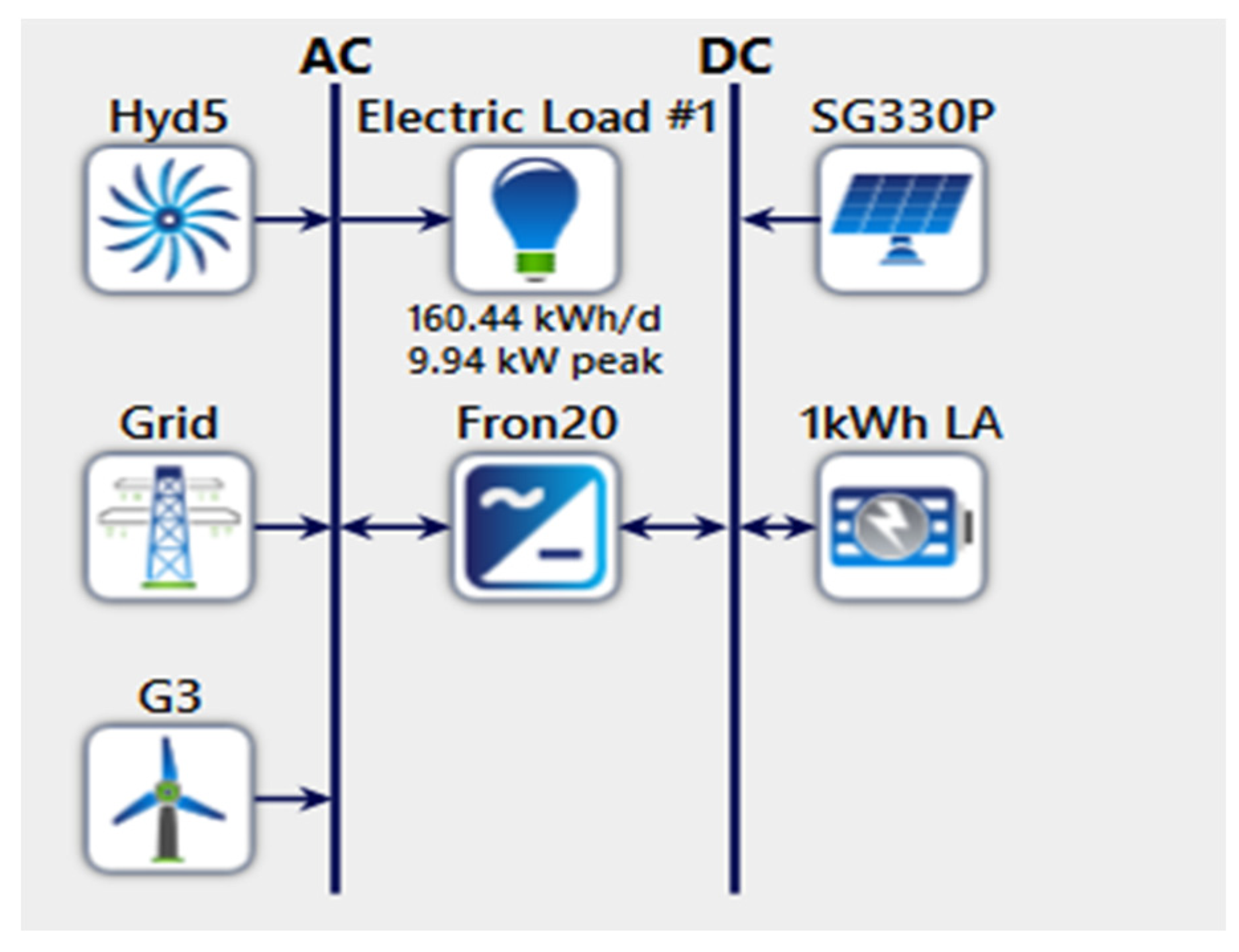
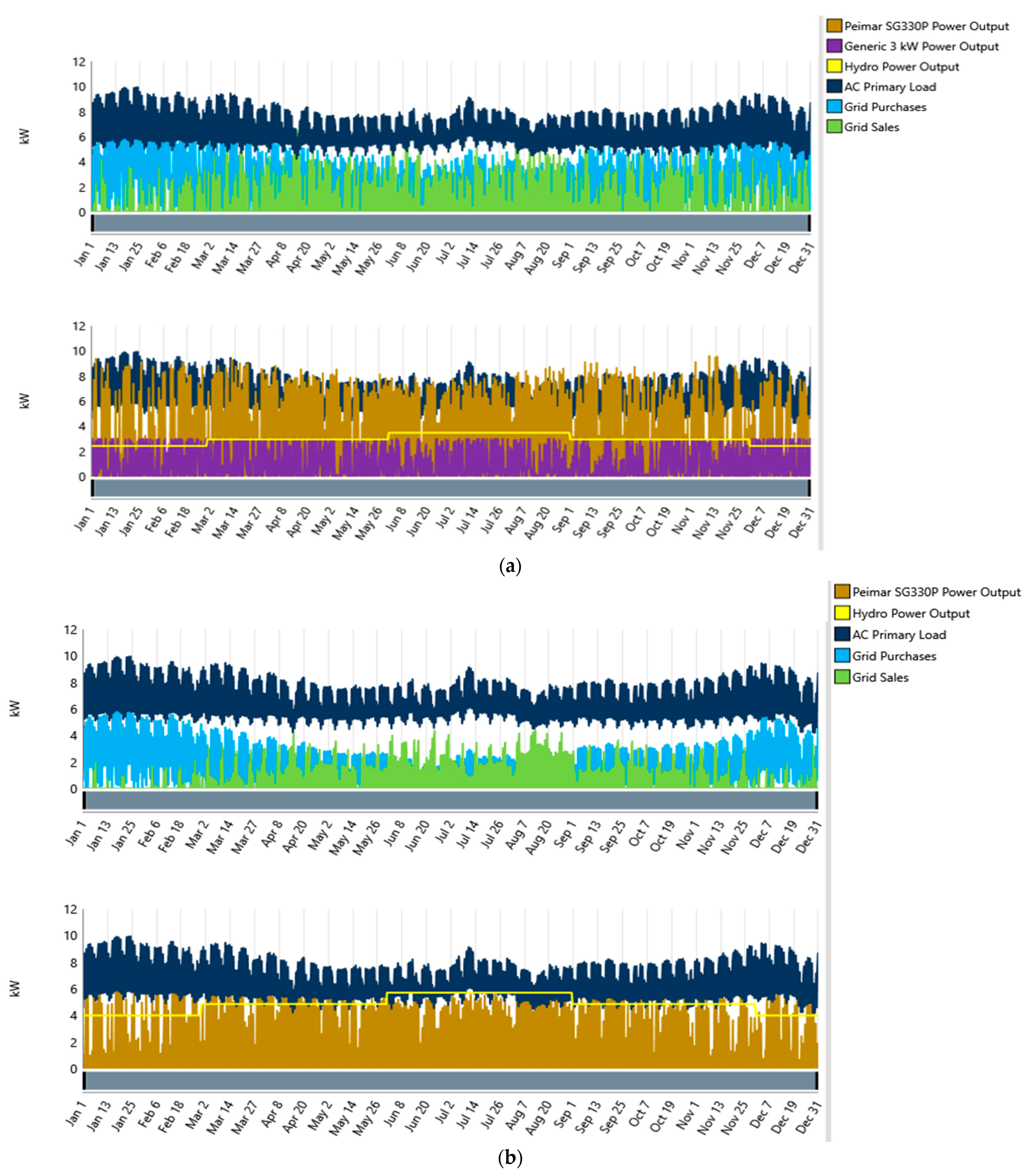
3.3. HOMER Simulation
- MP-02.5A-1: Illustration of the valve with the lowest flow value.
- SM04.5B: Identifies the valve with a flow value approximately equal to the average flow of all valves.
- TR08B: Designates the valve with the highest flow value.
4. Conclusions
- -
- Integrate micro-hydropower plants into water distribution systems, creating hybrid energy solutions.
- -
- Replace or add pressure control valves with PATs, allowing for clean power generation while maintaining pressure levels within certain limits.
- -
- Apply a real case study for an alternative solution, using the Funchal water network as an ideal case study for implementing this energy recovery method.
- -
- Demonstrate suitable locations for pressure-reducing valves (PRVs) and for the implementation of PATs.
- -
- A comprehensive analysis of the system’s operation to evaluate the economic feasibility of the investment.
- i.
- Variable-speed electrical regulation (ER) is preferable to a fixed-speed ER because it provides slightly higher performance for the exact equipment cost.
- ii.
- The “no regulation” mode (NR) is an unsuitable investment because it cannot adapt to fluctuating flow conditions, resulting in limited energy output.
- iii.
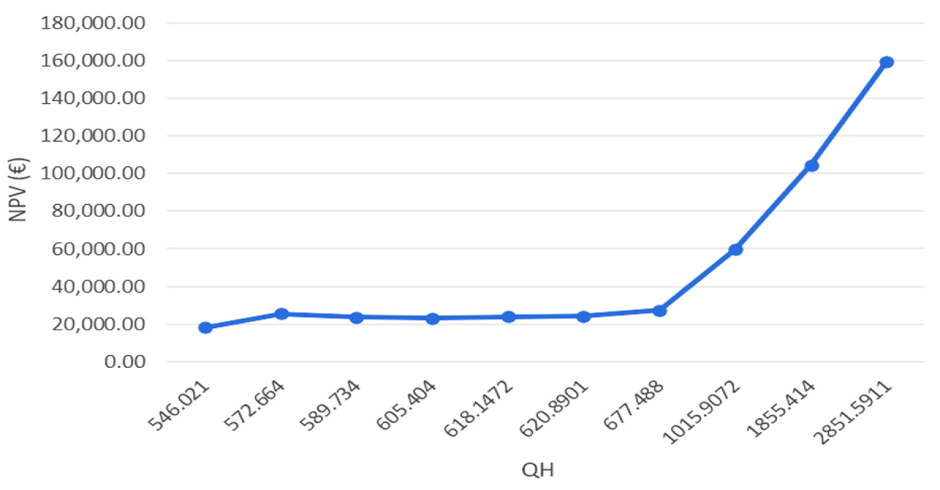
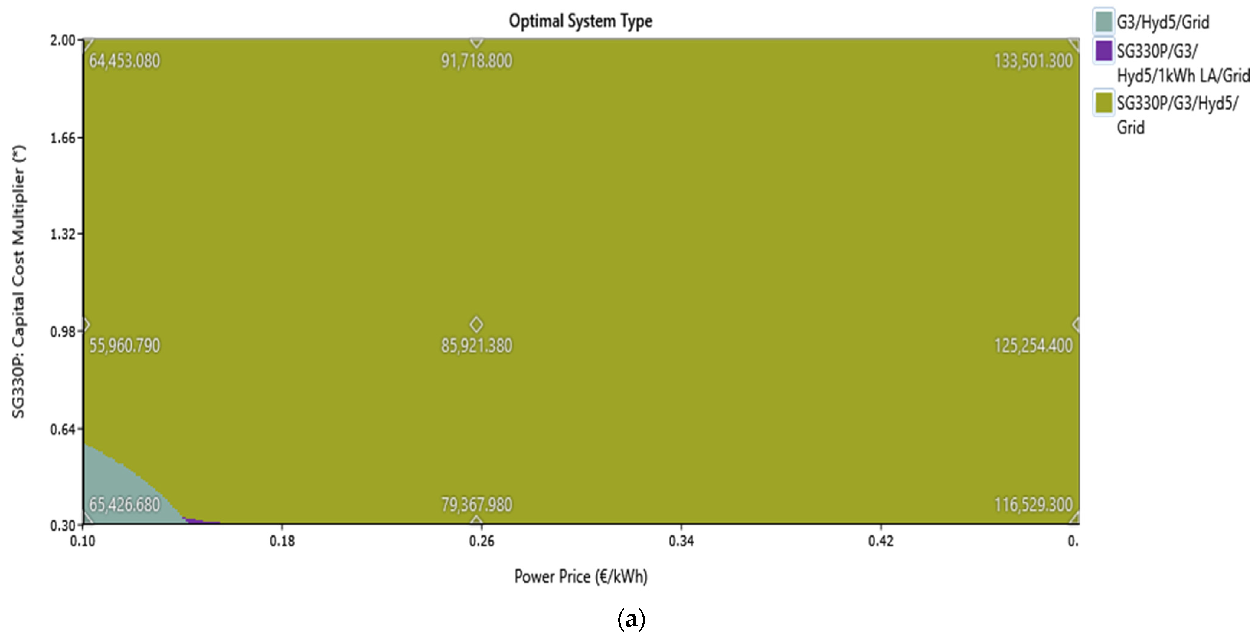
- Of the 50 newly implemented PRVs in Funchal’s water distribution system, only 10 PRVs were deemed viable for PAT. These PRVs together generate 406 MWh/year of energy, with a combined net present value.
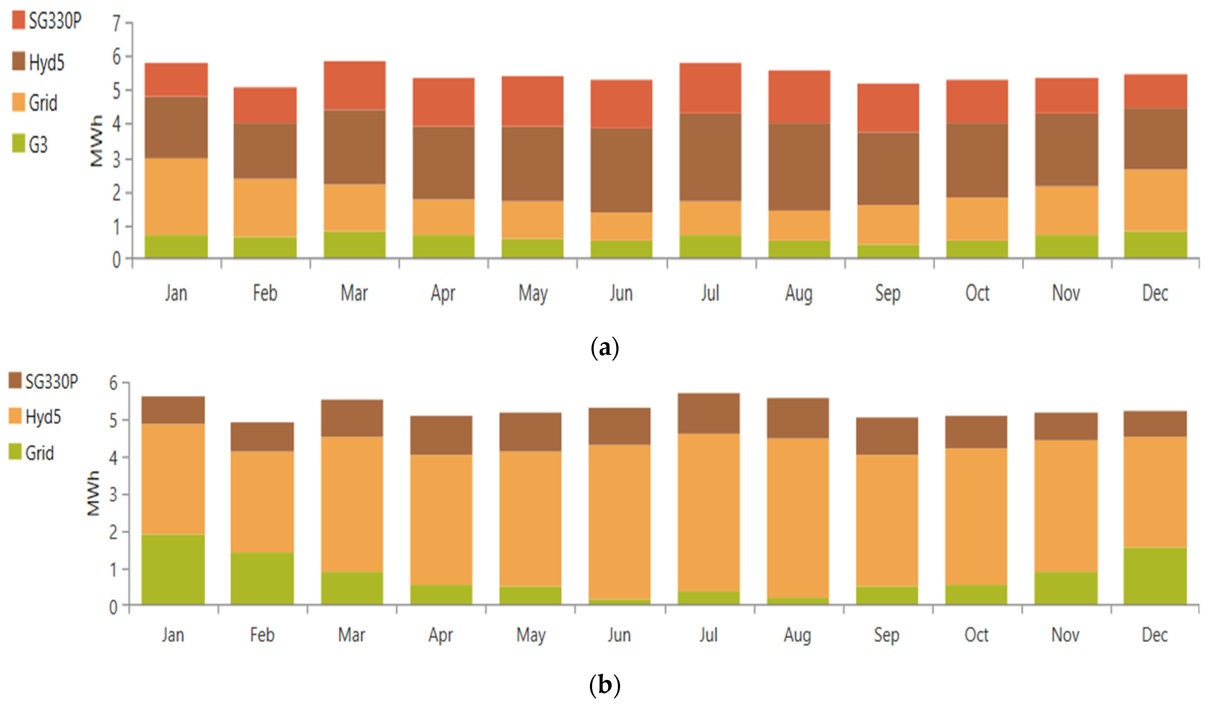
- i.
- Various PRVs were identified, and simulations were performed for each local system without changing the load and other power system specifications, such as capital, O&M, and replacement costs.
- ii.
- All simulations for all valves resulted in positive net present values, and additional analyses were performed to understand the nature of the economic benefits resulting from increased electricity generation from micro-hydro using PATs.
- iii.
- PV solar and micro-wind turbines installed in small DMAs in Funchal’s water distribution system produce 153 MWh/year and 55 MWh/year, respectively, adding to the 406 MWh/year generated by PATs. This adds up to 615 MWh/year at the ten selected PRV sites within Funchal’s water network alone.
Author Contributions
Funding
Data Availability Statement
Acknowledgments
Conflicts of Interest
References
- Sun, X.; Zhu, B.K.; Zhang, S.; Zeng, H.; Li, K.; Wang, B.; Dong, Z.F.; Zhou, C.C. New indices system for quantifying the nexus between economic-social development, natural resources consumption, and environmental pollution in China during 1978–2018. Sci. Total Environ. 2022, 804, 150180. [Google Scholar] [CrossRef] [PubMed]
- Chau, K.Y.; Moslehpour, M.; Tu, Y.T.; Tai, N.T.; Tien, N.H.; Huy, P.Q. Exploring the impact of green energy and consumption on the sustainability of natural resources: Empirical evidence from G7 countries. Renew. Energy 2022, 196, 1241–1249. [Google Scholar] [CrossRef]
- Guo, Y.; Uhde, H.; Wen, W. Uncertainty of energy consumption and CO2 emissions in the building sector in China. Sustain. Cities Soc. 2023, 97, 104728. [Google Scholar] [CrossRef]
- Sandri, S.; Hussein, H.; Alshyab, N. Sustainability of the Energy Sector in Jordan: Challenges and Opportunities. Sustainability 2020, 12, 10465. [Google Scholar] [CrossRef]
- Oberascher, M.; Rauch, W.; Sitzenfrei, R. Towards a smart water city: A comprehensive review of applications, data requirements, and communication technologies for integrated management. Sustain. Cities Soc. 2022, 76, 103442. [Google Scholar] [CrossRef]
- Pahl-Wostl, C.; Vörösmarty, C.; Bhaduri, A.; Bogardi, J.; Rockström, J.; Alcamo, J. Towards a sustainable water future: Shaping the next decade of global water research. Curr. Opin. Environ. Sustain. 2013, 5, 708–714. [Google Scholar] [CrossRef]
- Russo, T.; Alfredo, K.; Fisher, J. Sustainable water management in urban, agricultural, and natural systems. Water 2014, 6, 3934–3956. [Google Scholar] [CrossRef]
- Wakeel, M.; Chen, B.; Hayat, T.; Alsaedi, A.; Ahmad, B. Energy consumption for water use cycles in different countries: A review. Appl. Energy 2016, 178, 868–885. [Google Scholar] [CrossRef]
- Luderer, G.; Madeddu, S.; Merfort, L.; Ueckerdt, F.; Pehl, M.; Pietzcker, R.; Rottoli, M.; Schreyer, F.; Bauer, N.; Baumstark, L.; et al. Impact of declining renewable energy costs on electrification in low-emission scenarios. Nat. Energy 2022, 7, 32–42. [Google Scholar] [CrossRef]
- Sawle, Y.; Gupta, S.C.; Bohre, A.K. Review of hybrid renewable energy systems with comparative analysis of off-grid hybrid system. Renew. Sustain. Energy Rev. 2018, 81, 2217–2235. [Google Scholar] [CrossRef]
- Javed, M.S.; Zhong, D.; Ma, T.; Song, A.; Ahmed, S. Hybrid pumped hydro and battery storage for renewable energy based power supply system. Appl. Energy 2020, 257, 114026. [Google Scholar] [CrossRef]
- Das, P.; Das, B.K.; Mustafi, N.N.; Sakir, M.T. A review on pump-hydro storage for renewable and hybrid energy systems applications. Energy Storage 2021, 3, e223. [Google Scholar] [CrossRef]
- Erdinc, O.; Uzunoglu, M. Optimum design of hybrid renewable energy systems: Overview of different approaches. Renew. Sustain. Energy Rev. 2012, 16, 1412–1425. [Google Scholar] [CrossRef]
- Khatib, T.; Mohamed, A.; Sopian, K. A review of photovoltaic systems size optimization techniques. Renew. Sustain. Energy Rev. 2013, 22, 454–465. [Google Scholar] [CrossRef]
- Baños, R.; Manzano-Agugliaro, F.; Montoya, F.G.; Gil, C.; Alcayde, A.; Gómez, J. Optimization methods applied to renewable and sustainable energy: A review. Renew. Sustain. Energy Rev. 2011, 15, 1753–1766. [Google Scholar] [CrossRef]
- Chan, A.L.S. Generation of typical meteorological years using genetic algorithm for different energy systems. Renew. Energy 2016, 90, 1–13. [Google Scholar] [CrossRef]
- Lorestani, A.; Ardehali, M.M. Optimization of autonomous combined heat and power system including PVT, WT, storages, and electric heat utilizing novel evolutionary particle swarm optimization algorithm. Renew. Energy 2018, 119, 490–503. [Google Scholar] [CrossRef]
- Moosavian, S.M.; Modiri-Delshad, M.; Rahim, N.A.; Selvaraj, J. Imperialistic competition algorithm: Novel advanced approach to optimal sizing of hybrid power system. J. Renew. Sustain. Energy 2013, 5, 053141. [Google Scholar] [CrossRef]
- Dehghan, S.; Kiani, B.; Kazemi, A.; Parizad, A. Optimal sizing of a hybrid wind/PV plant considering reliability indices. World Acad. Sci. Eng. Technol. 2009, 56, 527–535. [Google Scholar]
- Askarzadeh, A. Distribution generation by photovoltaic and diesel generator systems: Energy management and size optimization by a new approach for a stand-alone application. Energy 2017, 122, 542–551. [Google Scholar] [CrossRef]
- Hadidian-Moghaddam, M.J.; Arabi-Nowdeh, S.; Bigdeli, M. Optimal sizing of a stand-alone hybrid photovoltaic/wind system using new grey Wolf optimizer considering reliability. J. Renew. Sustain. Energy 2016, 8, 035903. [Google Scholar] [CrossRef]
- Kaabeche, A.; Diaf, S.; Ibtiouen, R. Firefly-inspired algorithm for optimal sizing of renewable hybrid system considering reliability criteria. Sol. Energy 2017, 155, 727–738. [Google Scholar] [CrossRef]
- Maleki, A.; Pourfayaz, F.; Rosen, M.A. A novel framework for optimal design of hybrid renewable energy-based autonomous energy systems: A case study for Namin, Iran. Energy 2016, 98, 168–180. [Google Scholar] [CrossRef]
- Maleki, A.; Pourfayaz, F. Optimal sizing of autonomous hybrid photovoltaic/wind/battery power system with LPSP technology by using evolutionary algorithms. Sol. Energy 2015, 115, 471–483. [Google Scholar] [CrossRef]
- Maleki, A.; Askarzadeh, A. Artificial bee swarm optimization for optimum sizing of a stand-alone PV/WT/FC hybrid system considering LPSP concept. Sol. Energy 2014, 107, 227–235. [Google Scholar] [CrossRef]
- Sedighizadeh, M.; Esmaili, M.; Esmaeili, M. Application of the hybrid Big Bang-Big Crunch algorithm to optimal reconfiguration and distributed generation power allocation in distribution systems. Energy 2014, 76, 920–930. [Google Scholar] [CrossRef]
- Shezan, S.K.A.; Julai, S.; Kibria, M.A.; Ullah, K.R.; Saidur, R.; Chong, W.T.; Akikur, R.K. Performance analysis of an off-grid wind-PV (photovoltaic)-diesel-battery hybrid energy system feasible for remote areas. J. Clean. Prod. 2016, 125, 121–132. [Google Scholar] [CrossRef]
- Ramos, H.M.; Zilhao, M.; López-Jiménez, P.A.; Pérez-Sánchez, M. Sustainable water-energy nexus in the optimization of the BBC golf-course using renewable energies. Urban Water J. 2019, 16, 215–224. [Google Scholar] [CrossRef]
- Mercedes Garcia, A.V.; Sánchez-Romero, F.J.; López-Jiménez, P.A.; Pérez-Sánchez, M. A new optimization approach for the use of hybrid renewable systems in the search of the zero net energy consumption in water irrigation systems. Renew. Energy 2022, 195, 853–871. [Google Scholar] [CrossRef]
- García, A.V.M.; Sánchez-Romero, F.-J.; López-Jiménez, P.A.; Pérez-Sánchez, M. Is it possible to develop a green management strategy applied to water systems in isolated cities? An optimized case study in the Bahamas. Sustain. Cities Soc. 2022, 85, 104093. [Google Scholar] [CrossRef]
- Sowby, R.B. Correlation of Energy Management Policies with Lower Energy Use in Public Water Systems. J. Water Resour. Plan. Manag. 2018, 144, 06018007. [Google Scholar] [CrossRef]
- Wu, D.; Fan, G.; Duan, Y.; Liu, A.; Zhang, P.; Guo, J.; Lin, C. Collaborative optimization method and energy-saving, carbon-abatement potential evaluation for nearly-zero energy community supply system with different scenarios. Sustain. Cities Soc. 2023, 91, 104428. [Google Scholar] [CrossRef]
- Lode, M.L.; Felice, A.; Martinez Alonso, A.; De Silva, J.; Angulo, M.E.; Lowitzsch, J.; Coosemans, T.; Ramirez Camargo, L. Energy communities in rural areas: The participatory case study of Vega de Valcarce, Spain. Renew. Energy 2023, 216, 119030. [Google Scholar] [CrossRef]
- Dorahaki, S.; Rashidinejad, M.; MollahassaniPour, M.; Pourakbari Kasmaei, M.; Afzali, P. A sharing economy model for a sustainable community energy storage considering end-user comfort. Sustain. Cities Soc. 2023, 97, 104786. [Google Scholar] [CrossRef]
- Laske, S.; Paudel, A.; Scheibelhofer, O.; Sacher, S.; Hoermann, T.; Khinast, J.; Kelly, A.; Rantannen, J.; Korhonen, O.; Stauffer, F.; et al. A review of PAT strategies in secondary solid oral dosage manufacturing of small molecules. J. Pharm. Sci. 2017, 106, 667–712. [Google Scholar] [CrossRef] [PubMed]
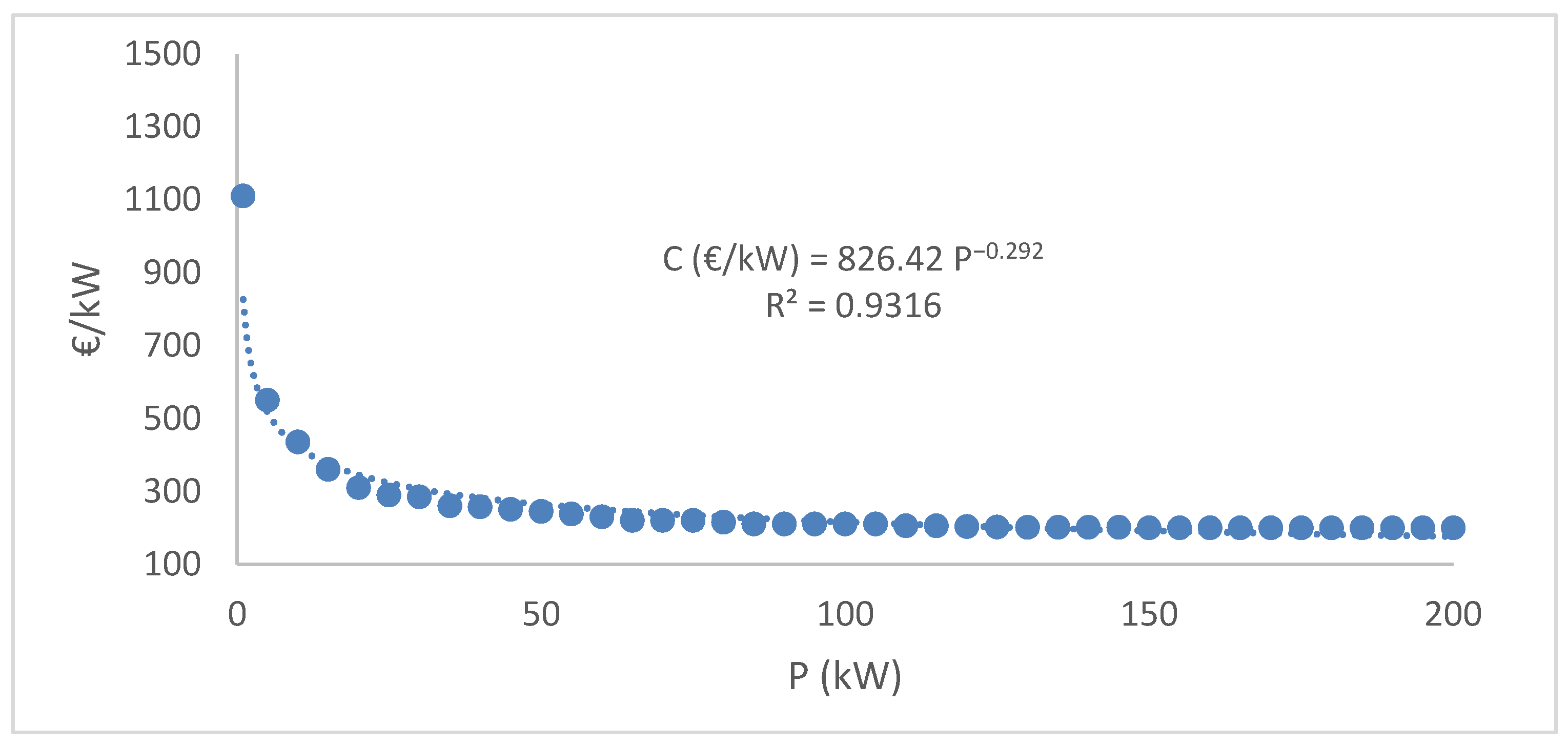
- Novara, D.; Fecarotta, O.; Carravetta, A.; Derakhshan, S.; McNabola, A.; Ramos, H.M. Pumps as Turbines (PATs) Cost Determination and Feasibility Study of Pressure Reducing Valve Substitution or Replacement with a PAT in a Water Supply System. 2016. Available online: https://www.semanticscholar.org/paper/Cost-Model-for-Pumps-as-Turbines-in-Run-of-River-Novara-Carravetta/4fd88fce3444f22ca4bd0ed700772312d1c2fb96 (accessed on 16 January 2024).
- Alberizzi, J.C.; Renzi, M.; Righetti, M.; Pisaturo, G.R.; Rossi, M. Speed and pressure controls of pumps-as-turbines installed in branch of water-distribution network subjected to highly variable flow rates. Energies 2019, 12, 4738. [Google Scholar] [CrossRef]
- Carravetta, A.; Fecarotta, O.; Del Giudic, G.; Ramos, H. Energy recovery in water systems by PATs: A comparisons among the different installation schemes. Procedia Eng. 2014, 70, 275–284. [Google Scholar] [CrossRef]
- Nautiyal, H.; Varun; Kumar, A. Reverse running pumps analytical, experimental and computational study: A review. Renew. Sustain. Energy Rev. 2010, 14, 2059–2067. [Google Scholar] [CrossRef]
- Derakhshan, S.; Nourbakhsh, A. Experimental study of characteristic curves of centrifugal pumps working as turbines in different specific speeds. Exp. Therm. Fluid Sci. 2008, 32, 800–807. [Google Scholar] [CrossRef]
- Derakhshan, S.; Nourbakhsh, A. Theoretical, numerical and experimental investigation of centrifugal pumps in reverse operation. Exp. Therm. Fluid Sci. 2008, 32, 1620–1627. [Google Scholar] [CrossRef]
- Energy Market Information System. Available online: https://mercado.ren.pt/EN/Gas/MarketInfo/Load/Actual/Pages/Hourly.aspx (accessed on 10 April 2023).
- Novara, D.; Carravetta, A.; Mcnabola, A.; Ramos, H.M. ‘A Cost Model for Pumps as Turbines in Run-off-River and in-Pipe Micro-Hydropower Applications’. J. Water Resour. Plan. Manag. 2018, 145, 04019012. [Google Scholar] [CrossRef]
- Ferreira, A.R. Energy Recovery in Water Distribution Networks towards Smart Water Grids. Master’s Thesis, IST Instituto Superior Tecnico de Lisboa Lisboa, Lisbon, Portugal, 2017. [Google Scholar]
- Chhipi-Shrestha, G.; Hewage, K.; Sadiq, R. Economic and energy efficiency of net-zero water communities: System dynamics analysis. J. Sustain. Water Built Environ. 2018, 4, 04018006. [Google Scholar] [CrossRef]
- Crosson, C.; Achilli, A.; Zuniga-Teran, A.A.; Mack, E.A.; Albrecht, T.; Shrestha, P.; Boccelli, D.L.; Cath, T.Y.; Daigger, G.T.; Duan, J.; et al. Net zero urban water from concept to applications: Integrating natural, built, and social systems for responsive and adaptive solutions. ACS ES&T Water 2020, 1, 518–529. [Google Scholar]
- Joustra, C.M.; Yeh, D.H. Framework for net-zero and net-positive building water cycle management. Build. Res. Inf. 2015, 43, 121–132. [Google Scholar] [CrossRef]
- Koirala, B.P.; Koliou, E.; Friege, J.; Hakvoort, R.A.; Herder, P.M. Energetic communities for community energy: A review of key issues and trends shaping integrated community energy systems. Renew. Sustain. Energy Rev. 2016, 56, 722–744. [Google Scholar] [CrossRef]
- Lowitzsch, J.; Hoicka, C.E.; van Tulder, F.J. Renewable energy communities under the 2019 European Clean Energy Package–Governance model for the energy clusters of the future? Renew. Sustain. Energy Rev. 2020, 122, 109489. [Google Scholar] [CrossRef]
- Zhang, C.Y.; Oki, T. Water pricing reform for sustainable water resources management in China’s agricultural sector. Agric. Water Manag. 2023, 275, 108045. [Google Scholar] [CrossRef]


| Component | Capital Cost | Replacement Cost | O&M Cost |
|---|---|---|---|
| Solar PV (SG330P) | 1000 EUR/kW | 1000 EUR/kW | 30 EUR/year |
| Wind turbine (G3) | 18,000 EUR/unit | 18,000 EUR/unit | 180 EUR/year |
| Battery 1kWh lead acid | 300 EUR/unit | 300 EUR/unit | 10 EUR/year |
| Inverter | 2500 EUR/unit | 2500 EUR/unit | 20 EUR/year |
| Hydro turbine (5 kW) | 2500 EUR/unit | 1250 EUR/unit | 500 EUR/year |
| Hydro turbine (10 kW) | 5000 EUR/unit | 2500 EUR/unit | 800 EUR/year |
| DN | EUR |
|---|---|
| 100 | 2260 |
| 300 | 8060 |
| 600 | 25,300 |
| 1260 | 55,838 |
| PRV (-) | D Pipe (mm) | D Valve (mm) | Q (L/s) | V (m/s) | Upstream Pressure (m) | Downstream Pressure (m) | Head Drop (m) | QH (-) |
|---|---|---|---|---|---|---|---|---|
| MP-03.5A-1 | 250FF | 150 | 32.20 | 1.82 | 44.75 | 23.71 | 21.04 | 6.64 |
| MP-02.5A-1 | 250FF | 150 | 20.66 | 1.17 | 52.27 | 22.35 | 29.92 | 6.06 |
| SM04.5A-1 | 200FF | 150 | 25.68 | 1.45 | 40.1 | 17.80 | 22.3 | 5.61 |
| SM04.5B | 200FF | 200 | 43.12 | 1.37 | 53.36 | 29.80 | 23.56 | 9.96 |
| RP04.5A | 250FC | 150 | 24.65 | 1.39 | 55.66 | 31.10 | 24.56 | 5.93 |
| TR08B | 500FF | 300 | 152.41 | 2.16 | 44.26 | 25.55 | 18.71 | 27.95 |
| TR07.5C | 200FF | 150 | 24.12 | 1.36 | 49.7 | 25.25 | 24.45 | 5.78 |
| TR06.5B | 200FF | 150 | 22.47 | 1.27 | 48.6 | 24.30 | 24.3 | 5.35 |
| TR05.5G | 200FF | 150 | 26.89 | 1.52 | 47.37 | 24.28 | 23.09 | 6.08 |
| TR07.5F | 400FF | 300 | 82.28 | 1.16 | 44.15 | 21.60 | 22.55 | 18.18 |
| PRV | PAT | Speed (rpm) | Emax (MWh) |
|---|---|---|---|
| MP-03.5A-1 | 65–250 | 1120 | 125.7 |
| MP-02.5A-1 | 65–250 | 770 | 34.3 |
| SM04.5A-1 | 65–250 | 1170 | 142.1 |
| SM04.5B | 65–250 | 1370 | 328.6 |
| RP04.5A | 65–250 | 1020 | 87.4 |
| TR08B | 100–200 | 1310 | 1005 |
| TR07.5C | 65–250 | 1070 | 111.7 |
| TR06.5B | 65–250 | 1020 | 87.9 |
| TR05.5G | 65–250 | 1170 | 149.9 |
| TR07.5F | 80–200 | 1470 | 686.7 |
| Valve | NPC of the Project (EUR) | LCOE of the Project (EUR/kWh) | Investment in Renewables (EUR) | Savings at 0.258 EUR/kWh Grid Price (EUR) | Net Present Savings (EUR) | ROI | NPV (EUR) |
|---|---|---|---|---|---|---|---|
| MP-03.5A-1 | 94,006.96 | 0.1157 | 47,461.05 | 313,869.90 | 74,701.04 | 0.574 | 27,239.99 |
| MP-02.5A-1 | 100,356.40 | 0.1227 | 49,507.50 | 308,155.20 | 73,340.94 | 0.481 | 23,833.44 |
| SM04.5A-1 | 108,988.70 | 0.1172 | 61,429.77 | 365,179.65 | 86,912.76 | 0.415 | 25,482.99 |
| SM04.5B | 52,401.24 | 0.0651 | 21,552.70 | 340,512.90 | 81,042.07 | 2.76 | 59,489.37 |
| RP04.5A | 101,947.40 | 0.1233 | 51,303.12 | 312,508.95 | 74,377.13 | 0.45 | 23,074.01 |
| TR08B | −4903.11 | −0.00342 | 15,342.01 | 714,414.90 | 174,933.86 | 10.083 | 159,591.85 |
| TR07.5C | 104,437.60 | 0.1214 | 54,795.61 | 329,782.05 | 78,488.13 | 0.432 | 23,692.52 |
| TR06.5B | 114,661.00 | 0.1259 | 66,552.13 | 355,891.65 | 84,702.21 | 0.273 | 18,150.08 |
| TR05.5G | 100,045.10 | 0.1225 | 49,081.53 | 307,426.35 | 73,167.47 | 0.491 | 24,085.94 |
| TR07.5F | 11,755.49 | 0.01186 | 15,342.01 | 487,878 | 116,114.96 | 6.568 | 104,359.47 |
| Valve | Q (l/s) | H (m) | QH | Solar PV SG330 P (kWh/yr) | Wind Turbine G3 (kWh/yr) | Hydro Output (kWh/yr) | Grid Purchase (kWh/yr) | LCOE of PAT (Hydro) |
|---|---|---|---|---|---|---|---|---|
| MP-03.5A-1 | 32.20 | 21.04 | 677.5 | 13,800 (21.4%) | 7915 (12.3%) | 28,421 (44%) | 14,455 (22.4%) | 0.0244 |
| MP-02.5A-1 | 20.66 | 29.92 | 618.1 | 15,690 (24%) | 7915 (12.1%) | 25,932 (39.7%) | 15,794 (24.2%) | 0.0267 |
| SM04.5A-1 | 25.68 | 22.30 | 572.6 | 25,025 (34.4%) | 7915 (10.9%) | 24,023 (33%) | 15,812 (21.7%) | 0.0289 |
| SM04.5B | 43.12 | 23.56 | 1015.9 | 11,066 (17.5%) | Not installed | 42,618 (67.3%) | 9680 (15.3%) | 0.0163 |
| RP04.5A | 24.65 | 24.56 | 605.4 | 17,680 (26.5%) | 7915 (11.8%) | 25,397 (38%) | 15,810 (23.7%) | 0.0273 |
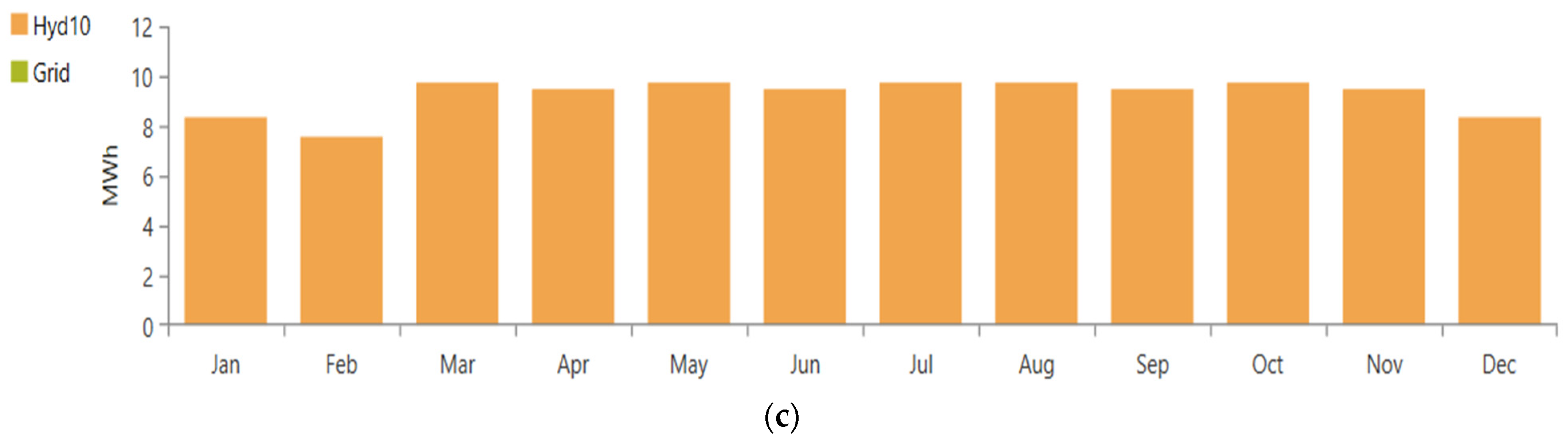
| TR08B | 152.41 | 18.71 | 2851.5 | Not installed | Not installed | 110,762 (100%) | Not purchased | 0.0107 |
| TR07.5C | 24.12 | 24.45 | 589.7 | 20,680 (29.9%) | 7915 (11.4%) | 24,740 (35.8%) | 15,813 (22.9%) | 0.0280 |
| TR06.5B | 22.47 | 24.30 | 546.0 | 34,436 (42.5%) | 7915 (9.76%) | 22,906 (28.3%) | 15,810 (19.5%) | 0.030 |
| TR05.5G | 26.89 | 23.09 | 620.8 | 15,137 (23.3%) | 7915 (12.2%) | 26,047 (40.1%) | 15,819 (24.4%) | 0.0266 |
| TR07.5F | 82.28 | 22.55 | 1851.3 | Not installed | Not installed | 75,640 (98.7%) | 1003 (1.31%) | 0.0157 |
| Energy System | Identification |
|---|---|
| G3 | Generic 3 kW wind turbine |
| Hyd5 | Generic 5 kW hydro turbine |
| SG330P | Solar PV |
| 1 kWh LA | Lead acid battery |
| Grid | Grid integration |
Disclaimer/Publisher’s Note: The statements, opinions and data contained in all publications are solely those of the individual author(s) and contributor(s) and not of MDPI and/or the editor(s). MDPI and/or the editor(s) disclaim responsibility for any injury to people or property resulting from any ideas, methods, instructions or products referred to in the content. |
© 2024 by the authors. Licensee MDPI, Basel, Switzerland. This article is an open access article distributed under the terms and conditions of the Creative Commons Attribution (CC BY) license (https://creativecommons.org/licenses/by/4.0/).
Share and Cite
Ramos, H.M.; Pérez-Sánchez, M.; Guruprasad, P.S.M.; Carravetta, A.; Kuriqi, A.; Coronado-Hernández, O.E.; Fernandes, J.F.P.; Branco, P.J.C.; López-Jiménez, P.A. Energy Transition in Urban Water Infrastructures towards Sustainable Cities. Water 2024, 16, 504. https://doi.org/10.3390/w16030504
Ramos HM, Pérez-Sánchez M, Guruprasad PSM, Carravetta A, Kuriqi A, Coronado-Hernández OE, Fernandes JFP, Branco PJC, López-Jiménez PA. Energy Transition in Urban Water Infrastructures towards Sustainable Cities. Water. 2024; 16(3):504. https://doi.org/10.3390/w16030504
Chicago/Turabian StyleRamos, Helena M., Modesto Pérez-Sánchez, Prajwal S. M. Guruprasad, Armando Carravetta, Alban Kuriqi, Oscar E. Coronado-Hernández, João F. P. Fernandes, Paulo J. Costa Branco, and Petra Amparo López-Jiménez. 2024. "Energy Transition in Urban Water Infrastructures towards Sustainable Cities" Water 16, no. 3: 504. https://doi.org/10.3390/w16030504
APA StyleRamos, H. M., Pérez-Sánchez, M., Guruprasad, P. S. M., Carravetta, A., Kuriqi, A., Coronado-Hernández, O. E., Fernandes, J. F. P., Branco, P. J. C., & López-Jiménez, P. A. (2024). Energy Transition in Urban Water Infrastructures towards Sustainable Cities. Water, 16(3), 504. https://doi.org/10.3390/w16030504