An Empirical Relation for Estimating Sediment Particle Size in Meandering Gravel-Bed Rivers

Abstract

This paper aims to obtain a relation for estimating the median size of bed sediment, $d_{50}$, at the bends of meandering rivers based on real data. To achieve such a purpose, field data, including topographic, sediment sampling, and flow measurements, were collected from various rivers in Iran at different times of the year. Then, the Buckingham Π-theorem was applied to identify the effective dimensionless numbers such as the Shields function, Reynolds particle number, Froude number, submerged specific gravity of sediment, and aspect and curvature ratios. A correlation analysis was conducted between such factors to eliminate those dependent on others. In the following, three regression techniques, containing the power function approach, the General Additive Model (GAM), and the Multivariate Adaptive Regression Spline (MARS), were chosen to achieve the best relation. The obtained results indicated that the developed MARS model produced a better result than the others and was much more satisfactory, with a coefficient of determination (R²) of 0.96 and 0.95 and Root-Mean-Square Error (RMSE) of 140.64 and 140.47 for the training and testing phases, respectively. Furthermore, the MARS outputs were validated with an analytical method, which showed that MARS fitted with the field data much better. Consequently, the distinguished merit of this study is the development of a relation for determining $d_{50}$ that shows which geometric and hydraulic parameters have the most effect on sediment size in the river bend.

1. Introduction

Determining the sediment particle size in alluvial rivers is essential for many purposes, such as sediment transport mechanisms [1], prediction of river morphodynamics [2], estimation of bed roughness [3], and maintenance of ecological conditions [4]. One of the few studies conducted is related to Bridge’s work in 1977, which established the median grain size of bed sediments in bends using the balance between the forces acting on grains. Although analytical relations are presented for both circular and non-circular bends separately in this study, the geometric characteristics of the bends are not directly presented in the relations [5]. In another study by Odgard in 1984, the grain size was studied in the bed’s armor layer, which ended in an analytical method with a relation. Such a study was compared with the data collected by other scientists [6,7]. However, the main focus of the current research has been on the size distribution of sediment particles in the armor layer in non-meandering beds. Julien and Anthony used a three-dimensional approach to determine the direction of particles in motion with different sizes in natural meander bends [8]. Also, the work of Wright and Parker using the numerical finite difference method with field data established a one-dimensional mathematical formulation for downstream fining in sand-bed rivers [9]. Jang et al. studied the effects of lifting force on bed sediment size using a numerical model in another investigation. The outcome showed that the consequences of the mentioned force were significant [10]. Kuhnle et al. surveyed the impact of bed shear stress on the bed grain size distribution with a poorly sorted combination of sand and gravel. They proved the increasing of the bed median sediment size with bed shear stress [11]. In a series of experiments by McKie et al., the various distance effects of stabilized large sediment particles on the bed and transported sediment sizes in gravel-bed rivers were investigated. The results reflected that reducing the spaces between the particles made the transported and bed sediment sizes coarser [12]. White and Nelson used a sinusoidal flume with constant flow rates to study the mechanisms influencing sediment sorting patterns in a channel bed. They reported that interactions between channel shape, bed topography, and secondary currents led to fine and coarse sediment deposition on bars and pools, respectively [13].

Additionally, some research has used traditional regression approaches to predict the relation between the distribution of sediment particles and other hydraulic variables. Yen and Lee formulated transverse sediment sorting in a laboratory channel bend under unsteady flow conditions and determined a regression equation for the variation of sediment size [14]. Pitlick et al. expressed a regression relation for grain size in bed surface and substrate layers with flow properties in gravel-bed rivers [15]. Also, using the least squares linear regression method, Naito et al. set out a study about a total bed material relation for a fine sediment mixture to treat grain sorting in sand–silt bed rivers [16]. However, these techniques may need to be more efficient to fully explain the effect of channel geometry variables and flow parameters in an alluvial channel [17].

On the other hand, various advanced models like Generalized Additive Model (GAM), Multivariate Adaptive Regression Spline (MARS), Support Vector Machine (SVM), and such have been used for different hydraulically and hydrologically matters [18,19,20,21,22]. Among these, GAM and MARS sound fairly comprehensive to expand a set of formulas for estimating the particle sediment size in bends. Recently, these techniques have been successfully used to present a variety of subjects related to flow and sediment dynamics [23,24]. Each regression model has its own strengths and weaknesses; for example, although the power model errors may increase with multi-collinearity between the parameters, it is one of the best among the other traditional ones to predict the behavior of natural phenomena. Also, the GAM interpretation results may be challenging due to the complexity of their functions. However, it applies smooth functions to the predictor variables instead of describing a quantity as a linear or polynomial function [25]. Regarding MARS, it is a flexible method with optimal accuracy compared to the other techniques to clarify outputs using linear and nonlinear relations [26]. Not only does MARS create nonparametric modeling without using functional equations between inputs and outputs to recognize the effect of relevant parameters, but it also selects essential variables automatically to predict the results with a high analytical speed in comparison with the other techniques [27]. The superiority of the MARS model is that its structure is additive and interactive, creating fewer variable interactions and fewer deviations [28].

Despite conducting numerous studies on the sediment dynamics in natural meandering bends, it is impossible to predict with certainty what parameters of the bend and which elements of flow characteristics can affect the size of the bed sediment particles. Also, there are some questions, such as whether there is a relation between the size of the bed sediment particles as well as the large-scale components of the bend and flow characteristics, or whether it is possible to estimate the size of these particles under the influence of bend physical specifications. So, calculating sediment particle sizes, especially in meandering rivers, requires more attention and is a fundamental goal of sediment studies. For this reason, this study focused on estimating the median particle size of sediments in alluvial gravel beds, and attempts were made to find a reliable relation between the channel bend geometry and the flow characteristics. To achieve this aim, field measurements were made to collect data in the natural meandering rivers. In addition, dimensional analysis was applied to diminish the number of variables involved and to introduce a nondimensional framework based on the physical insight of the problem and the results of other previously conducted research. Then, three regression forms—the power model as a classical one, GAM, and MARS as advanced techniques—were adopted to develop a mathematical relation between parameters obtained from the dimensional analysis to choose the best-fitted model using the R programming package v.4.3.2 [29]. Furthermore, the outputs were compared, and the results of the superior model were evaluated with Bridge’s analytical relation. Finally, parameter sensitivity and uncertainty analysis were employed to understand the trend of the superior model estimations and ensure the robustness of this one.

Collecting the field data and identifying the effective parameters can strengthen this study and provide a reliable understanding of this issue. Additionally, developing an empirical relation to determining the median size of sediment particles using three different regression models and presenting the best model can help fill such a gap. Validation of outputs with the analytical model can establish acceptable trust in the model and its results.

2. Materials and Methods

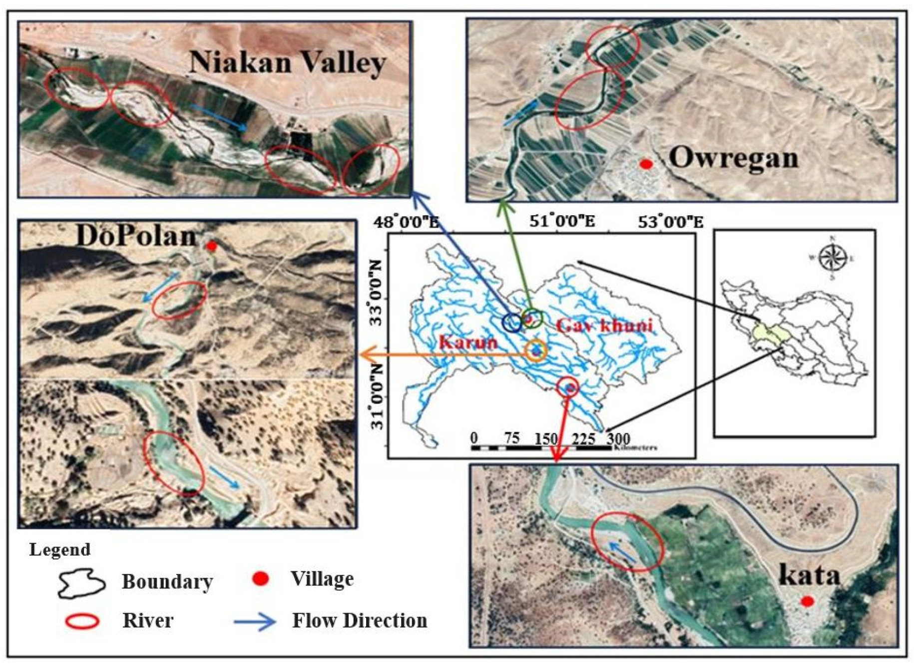
2.1. Field Measurements

A number of 187 sediment samples were collected from different reaches of four meandering rivers named the Niakan, Zayandehrood, Karun, and Khersan in Chaharmahal Va Bakhtiari and Koohkelooyeh Va BoyerAhmad, the provinces of Iran. The sampling sites were selected based on availability, and the bed materials ranged from different gravel sizes. Moreover, no regulatory structures or human activities were accessible up to 10 times the bankfull width from upstream and downstream reaches. Accordingly, nine free bends with different curvature radii were considered, four of which were located in the Niakan River in Niakan valley (50°09′06″ E, 32°31′52″ N & 50°09′11″ E, 32°31′33″ N), two in the Zayandehrood in the vicinity of Owregan village (50°25′33″ E, 32°36′18″ N), two in the Karun near DoPolan region (50°35′50″ E, 31°54′31″ N & 50°37′21″ E, 31°52′31″ N), and one in the Khersan downstream of Kata village (51°15′30″ E, 31°11′05″ N). Figure 1 shows the locations of the study areas.

To gather bed-surface sediments and flow data, a minimum of three and a maximum of five cross-sections for each river were chosen based on the dimensions of the bends. However, one or two extra cross-sections were considered for accuracy in large bends. Cross-sections were surveyed by dividing them into several subsections, each ranging from 0.5 to 6 m. Following that, from the beginning to the end of each interval, bed samples were gathered into 200 pebbles lying to a depth of up to 1.97 m. Simultaneously, water depth and flow velocity (streamwise component) were recorded at each sampling point along the cross-sections. A current meter (Ab Andishan Zayandehrood, Isfahan, Iran) with the capability of flow velocity measurement in the 0.05 to 5 m/s range with an accuracy of ±0.1% to ±5% was used to gain the water velocity.

Also, surveying was undertaken using multi-frequency G.P.S. and total station instruments (Ruide Surveying Instrument Co. Ltd., Guangzhou, China) to obtain the topographic data of the river bends by two sets of measurements along the water surface and floodplain. The distance between the surrounding points was determined to be between 0.5 and 1 m to accurately record the geometry of the bends (about 2000 points for each bend on average). Field collection of data and sampling were conducted in the rivers in October, November 2019, and May 2020.

In the next step, after drying, all the sediment samples were sieved and weighed based on laboratory methods, using mechanical sieving, submerged, and direct shear tests to characterize median grain sizes ($d_{50}),$ Specific Gravity ($SG$), and internal friction angle ($\phi )$. The point sample weights ranged from approximately 120 to 800 g, and all the samples were gravelly sediments based on Unified Soil Classification System (U.S.C.S.) [30].

Calculated flow parameters, including the average flow velocity and the bed shear stress, were determined regarding the mid-section method and consideration of the formula ${\tau }_{\mathrm{b}}{=\rho }_{w}g{R}_{h}S$, respectively, where ${\rho }_w$ shows the water density, $g$ stands for the acceleration of gravity, $R_h$ signifies the hydraulic radius, and $S$ is the energy slope. In addition, after processing geometric field data, the radius curvatures of the bends, $R_c$, were obtained by adjusting a circle on the center line of the bend. Similarly, the observed data via fundamental relations distinguished other flow-relevant and channel geometry variables.

Table 1. Range of the observed data and calculated parameters.

Variables	Units	Minimum	Maximum
Flow depth, $h$	m	0.15	1.97
Channel top width, $T$	m	3.60	58.5
Flow velocity, u	m/s	0.10	1.44
Mean sediment size, $d_{50}$	mm	15	53
Specific Gravity, $SG$	-	2.66	2.74
Angle of integral friction, 𝜑	°	24	32
Curvature radius, $R_c$	m	50	287
Longitudinal slope, γ	-	0.005	0.01
Transverse slope, α	-	0.0015	0.0075

summarizes the range of both the observed and calculated data.

Since the purpose is to calculate $d_{50}$ along the bend, the sediment characteristics in each cross-section, identical to the values of the flow parameters, were averaged and used in the dimensional analysis.

2.2. Dimensional Analysis

The bed sediment particle size in a river bend with a radius curvature of $R_c$, the cross-sectional mean flow velocity of $\overline{u}$, and the shear stress of ${\tau }_b$ were expressed by the following functional form:

$$f(T,R_c,D_h,d_{50},\overline{u},{\tau }_b,g,\mu ,{\rho }_w,{\rho }_s-{\rho }_w)=0,$$

(1)

where $T$ stands for channel top width, $D_h$ signifies hydraulic depth defined via dividing the flow area by channel top width $(D_h=\frac{A}{T})$. $d_{50}$ symbolizes median sediment grain size, ${\rho }_s$ mirrors sediment density, $\mu$ shows water dynamic viscosity, and $g$ and ${\rho }_w$ are the same parameters previously described.

The functional relation was obtained using the Buckingham Π-theorem [31] with the number of variables and the base quantities (i.e., length, time, and mass). The number of seven ${\mathsf{\Pi }}_{\mathrm{i}}$ obtained was generated by choosing ${\rho }_w,{\tau }_b$, and $d_{50}$ as repeated variables. The first dimensionless parameter (${\mathsf{\Pi }}_1$) was developed via dividing $T$ by $d_{50}$ (${\mathsf{\Pi }}_1=\frac{T}{d_{50}}$). This parameter introduces the median sediment particle size in a given section of the bend with a width of $T$. Changes in sediment size in river bends depend on cross-circulation motion related to the curvature ratio [32], so $\frac{R_c}{d_{50}}$ was selected as the second-dimensional group (${\mathsf{\Pi }}_2=\frac{R_c}{d_{50}}$), which can be changed to the curvature ratio via the combination with ${\mathsf{\Pi }}_1$; ${\mathsf{\Pi }}_2^{\prime }={\mathsf{\Pi }}_2\times {\mathsf{\Pi }}_1^{-1}=\frac{R_c}{T}$. It is also reported that the aspect ratio and submerged specific gravity can affect the sediment particle size [33]; thus, ${\mathsf{\Pi }}_3=\frac{D_h}{d_{50}}$ that can be changed to ${\mathsf{\Pi }}_3^{\prime }={\mathsf{\Pi }}_3^{-1}\times {\mathsf{\Pi }}_1=\frac{T}{D_h}$ and ${\mathsf{\Pi }}_4=\frac{{\rho }_s-{\rho }_w}{{\rho }_w}=SG-1$.

Another effective parameter produced by shear stress, ${\mathsf{\Pi }}_5=\frac{{\tau }_b}{{\rho }_{w}g{d}_{50}}$, can be converted to a new dimensionless group by division of ${\mathsf{\Pi }}_5$ and ${\mathsf{\Pi }}_4$ (${\mathsf{\Pi }}_5^{\prime }=\frac{{\tau }_b}{{\rho }_{w}g(SG-1)d_{50}}$) to obtain a known parameter presented as the Shields number, ${\theta }_{shields}.$ The following dimensionless developed parameter was ${\mathsf{\Pi }}_6=\frac{d_{50}\sqrt{{\rho }_w{\tau }_b}}{\mu }$, considering ${\tau }_b={\rho }_w{u}_{\mathrm{*}}^2$ and $\vartheta =\mu /{\rho }_w$, in which $u_{\mathrm{*}}$ is the shear velocity and $\vartheta$ is the water kinematic viscosity that equals ${10}^{-6} {\mathrm{m}}^2/\mathrm{s}$, simplified as ${\mathsf{\Pi }}_6^{\prime }=\frac{u_{\mathrm{*}}{d}_{50}}{\vartheta }$ named particle Reynolds number, $R_{e*}$.

The role of natural flow regimes introduced by another nondimensional group developed via ${\mathsf{\Pi }}_7=\frac{\overline{u}\sqrt{{\rho }_w}}{\sqrt{{\tau }_b}}$. This parameter, rewritten to another combined dimensionless group, ${\mathsf{\Pi }}_7^{\prime }={\left(\frac{{\mathsf{\Pi }}_7^2\times {\mathsf{\Pi }}_5}{{\mathsf{\Pi }}_3}\right)}^{1/2}$, led to the Froude number, $F_r=\frac{\overline{u}}{\sqrt{g{D}_h}}$.

By considering the mentioned dimensionless groups, the following functional relation can be expressed between the sediment particle size and the variables:

$$\frac{T}{d_{50}}=f^{\prime }\left(\frac{R_c}{T},\frac{T}{D_h},SG-1,{\theta }_{shields},R{e}_{\mathrm{*}},Fr\right)$$

(2)

where the values $R_c/T$, $T/D_h$, $SG-1$, ${\theta }_{shields}$, $R{e}_{\mathrm{*}}$, and $Fr$ are taken as input variables to determine $T/d_{50}$.

Since some parameters may depend on others, it is essential to figure out and omit them to ensure all the input variables are independent. So, the correlation analysis method was used to evaluate the data dependency.

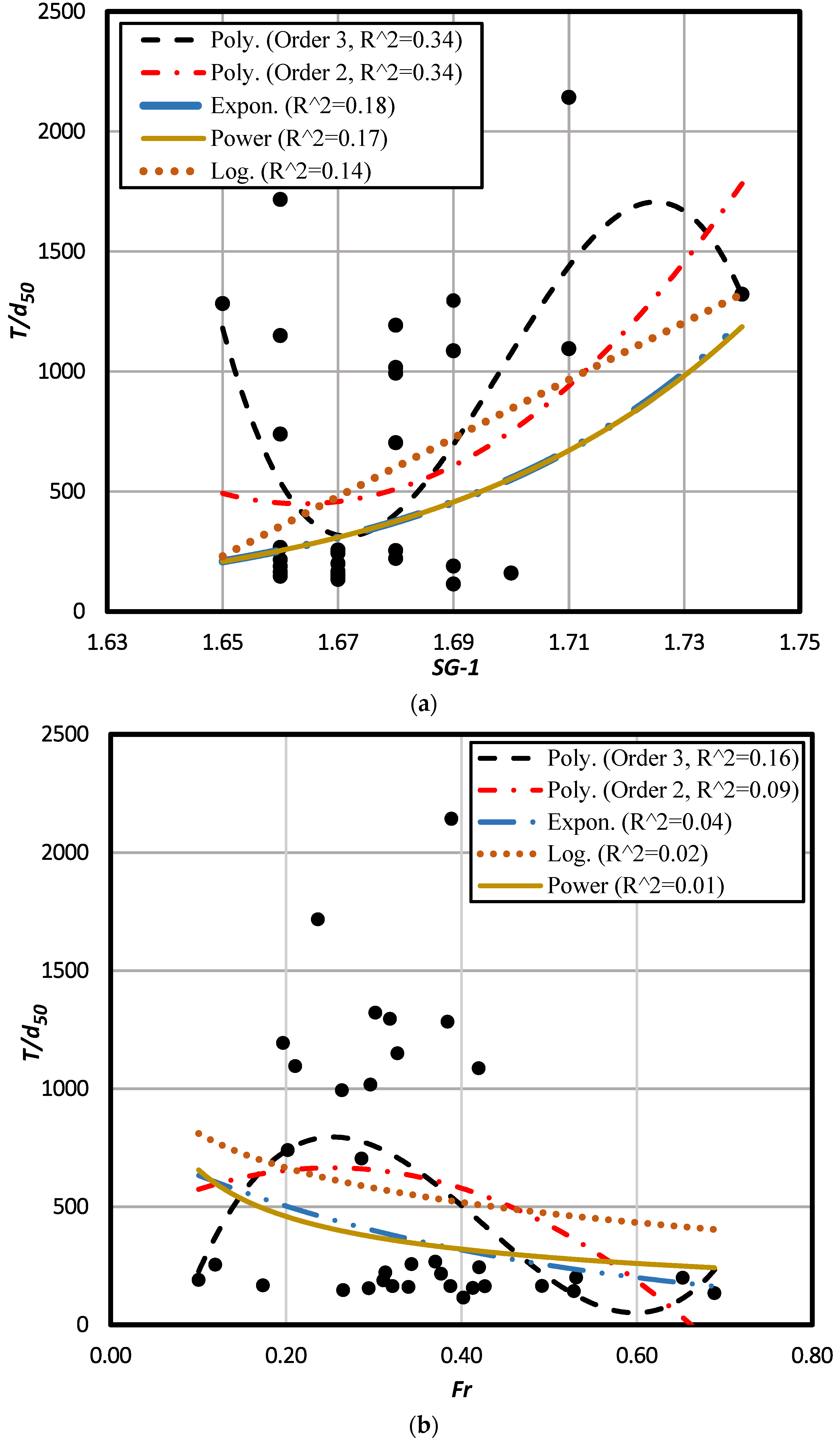
2.3. Correlation Analysis between Variables

Multicollinearity is a statistical event where independent variables in a regression model are highly correlated and cause an unrealistic model to be developed with incorrect results. The Bartlett sphericity test [34] was applied to survey the correlation between the parameters and eliminate highly correlated variables. In the first step, the p-value resulting from the test statistic was much less than the significant level ($\alpha$), equal to a value of 0.05, which indicated a dependency on the data. By using the correlation matrix, it was found that the maximum correlation factor was between $R{e}_{\mathrm{*}}$ and ${\theta }_{shields}$, with an r value of 79%. Therefore, $R{e}_{\mathrm{*}}$ was removed from the predictor variables.

Later, by reusing the test for the remaining variables, the p-value came to be 0.0003, which was also less than $\alpha$. In the correlation matrix, it was determined that the parameters $T/D_h$ and ${\theta }_{shields}$ had the highest correlation coefficient (r = 41%). Consequently, the variable $T/D_h$ was eliminated from the other parameters. By readjusting the test, the p-value was equal to 0.1256, more than $\alpha$. Thus, the assumption of data independence was established, and the final correlation coefficients between the variables were low enough, as shown in

Table 2. Final correlation coefficients between the independent variables (%).

Variables	$\mathit{S}\mathit{G}-1$	${\mathit{\theta }}_{\mathit{s}\mathit{h}\mathit{i}\mathit{e}\mathit{l}\mathit{d}\mathit{s}}$	${\mathit{R}}_{\mathit{c}}/\mathit{T}$	$\mathit{F}\mathit{r}$
$SG-1$	100	26	−30	−18
${\theta }_{shields}$	26	100	−23	−22
$R_c/T$	−30	−23	100	29
$Fr$	−18	−22	29	100

.

Accordingly, among the dimensionless groups, $SG-1$, ${\theta }_{shields}$, $R_c/T$, and $Fr$ were considered independent variables to develop the sediment particle size relation. Before using the regression models, the data were split into training and testing sets. There is no particular criterion for splitting, and researchers have used various segmentations between the data [35]. This study used a repeated random sub-sampling technique based on the splitting data with 50 iterations. The data are split into 75% for training and 25% for testing.

3. Results

3.1. Power Regression Model

Multivariate power regression is one of the most common methods applied in dimensional analysis [36]. It is expressed as:

$$y=c_0\prod _{i=1}^N{x}_i^{K_i}$$

(3)

where $y$ is a dependent output variable ($\frac{T}{d_{50}}$), $c_0$ displays a constant term, $x_i$ presents independent input variables (Table 2), $k_i$ clarifies the power of the $i\mathrm{t}\mathrm{h}$ term, and $N$ reflects a number of variables.

Fifteen combinations of the independent variables were considered using the power regression method, and they were evaluated by the Root-Mean-Square Error (RMSE) and the Mean Absolute Error (MAE) indices using the following expressions [37].

$$RMSE=\sqrt{\frac{{\sum }_{i=1}^n{\left(O_i-P_i\right)}^2}{n}}$$

(4)

$$MAE=\frac{{\sum }_{i=1}^n\left|O_i-P_i\right|}{n}$$

(5)

in which $O_i$ is the real value for ith observation, $P_i$ is the predicted value for ith observation, and $n$ is the number of observations.

The best combination, based on testing data, was related to $SG-1$, ${\theta }_{shields}$, $Fr$, and $R_c/T$ (

Table 3. The values of RMSE and MAE indices for different combinations of independent variables.

Combination of Independent Variables	RMSE		MAE
	Training	Testing	Training	Testing
$SG-1$	525.97	608.34	419.99	379.70
${\theta }_{shields}$	416.95	632.43	270.43	473.38
$Fr$	551.72	689.03	389.27	523.99
$R_c/T$	462.39	512.70	300.02	315.26
$SG-1$,${\theta }_{shields}$	582.82	407.16	252.70	441.27
$SG-1$, $Fr$	600.90	529.84	379.52	416.06
$SG-1$, $R_c/T$	436.20	556.10	284.49	364.76
${\theta }_{shields}$, $Fr$	409.28	580.50	262.30	398.90
${\theta }_{shields}$, $R_c/T$	325.61	440.31	224.85	329.45
$Fr$, $R_c/T$	456.88	515.11	291.77	310.20
$SG-1$, ${\theta }_{shields}$, $Fr$	369.94	541.79	254.82	392.73
$SG-1$, ${\theta }_{shields}$, $R_c/T$	311.40	365.47	214.74	281.36
${\theta }_{shields}$, $Fr,$$R_c/T$	301.26	386.83	200.28	271.23
$SG-1$, $Fr,$$R_c/T$	437.61	549.43	282.11	367.02
$SG-1$, ${\theta }_{shields}$,$Fr$, $R_c/T$	287.65	320.99	197.53	247.61

).

For the prominent combination, the RMSE and MAE values of the training data were 287.65 and 197.53, respectively, and the values for the testing data in rank were 320.99 and 247.61. The model showed sufficient accuracy in its predictions and can be described as follows:

$$\frac{T}{d_{50}}=0.96{\left(SG-1\right)}^{10.73}{\left({\theta }_{shields}\right)}^{-0.56}{\left(Fr\right)}^{-0.49}{\left(\frac{R_C}{T}\right)}^{-0.96}$$

(6)

In addition, sensitivity analysis was performed for the input variables using an analysis of variance (ANOVA) test to discover the significance of each parameter in the model [38]. As shown in

Table 4. p-values based on ANOVA test for each variable in power regression.

Variables	p-value	Result
$SG-1$	0.31230 > 0.05	No significant level
$Fr$	0.05 < 0.05448 < 0.1	Medium significant level
${\theta }_{shields}$	0.00021 < 0.001	High significant level
$R_c/T$	0.00002 ≪ 0.001	High significant level

, based on the p-value, it can be concluded that the ($SG-1)$ variable had no significant level. Therefore, it produced a minimum effect on Equation (6), so it could be ignored. The remaining variables $R_c/T$ and ${\theta }_{shields}$ had high and $F_r$ medium significant levels.

Accordingly, an optimum power relation for predicting sediment particle size could be re-expressed without the ($SG-1$) variable with a coefficient of determination (R²) of 0.81 (Equation (7)).

$$\frac{T}{d_{50}}=314.1{\left({\theta }_{shields}\right)}^{-0.53}{\left(Fr\right)}^{-0.51}{\left(\frac{R_C}{T}\right)}^{-1.03}$$

(7)

3.2. GAM Model

The Generalized Additive Model (GAM) is an algorithm based on generalizing a linear model with a series of predictors containing common features for each auxiliary variable, first introduced by Hastie and Tibshirani in 1990 [39]. This model has neither the complexity of advanced models nor the incompatibility of classical ones. Proper configuration of different functions in GAM may produce an accurate model more consistent with the data than the linear model [40]. Using nonparametric smoothing functions makes it possible to describe complex environmental phenomena adequately [23]. The basic form of the GAM model is represented by:

$$y=c_0+\sum _{i=1}^N{S}_i \left(x_i\right)$$

(8)

where $c_0$ reflects a constant term, $S_i \left(x_i\right)$ is different from the smooth functions, and N displays a number of variables.

Generally, the GAM optimum model has been developed by selecting the best normal function for each auxiliary variable versus the objective variable separately and adding them together [41]. Here, we used four primary function forms, namely polynomial, power, exponential, and logarithmic, to obtain the most appropriate model for each auxiliary variable. Then, the best-fitted function form was selected based on the R² value (Figure 2 and Figure 3).

Among the fitted functions, the polynomial form with degrees 2 and 3 seemed the best for $T/d_{50}$ versus $SG-1$. The value of R² for them was the same and almost equal to 0.34. Hence, the low-order polynomial function with degree 2 was picked as the best form.

A polynomial function with order 3 created the best match of $T/d_{50}$ versus ${\theta }_{shields}$ and $F_r$ with R² values of 0.87 and 0.16, respectively. Also, the best-fitted function for $T/d_{50}$ versus $R_c/T$ appeared to be the logarithmic form with the highest R² equal to 0.77.

Table 5. Best-matched functions for auxiliary variables in GAM regression model.

Variables	$\mathit{S}\mathit{G}-1$	$\mathit{F}\mathit{r}$	${\mathit{\theta }}_{\mathit{s}\mathit{h}\mathit{i}\mathit{e}\mathit{l}\mathit{d}\mathit{s}}$	${\mathit{R}}_{\mathit{c}}/\mathit{T}$
Best form	Polynomial	Polynomial	Polynomial	Logarithmic
Order	2	3	3	-
R2	0.34	0.16	0.87	0.77

shows the best-matched functions with the corresponding R² for each auxiliary variable.

Using the GAM model, the selected forms for each auxiliary variable were combined as an additive equation to create a single equation and predict the $T/d_{50}$ with (Equation (9)). The RMSE and MAE equal 390.79 and 375.32, respectively, for the test data set.

$$\begin{gathered} \frac{T}{d_{50}}\approx 979.763-220.184\times \mathit{log}\left(\frac{R_C}{T}\right)+f\left(F_r\right)+g\left({\theta }_{Shields}\right)+k\left(SG-1\right) \\ f\left(F_r\right)=F_r\times \left(-351.188+70.58\times F_r+411.418\times {F_r}^2\right) \\ g\left({\theta }_{Shields}\right)={\theta }_{Shields}\times \left(-771.595+827.056\times {\theta }_{Shields}-305.378\times {\theta }_{Shields}^2\right) \\ k \left(SG-1\right)=(SG-1)\times \left(672.23+534.36\times (SG-1)\right) \end{gathered}$$

(9)

In order to find the optimal combination of the variables (Equation (9)), the recursive elimination algorithm [42] was used to select the most effective variables so that $T/d_{50}$ could be predicted. This algorithm applied a backward selection process and removed the variable(s) of minor importance based on the model evaluation metric. Here, the ANOVA test was applied, and the $SG-1$ with a p-value equal to 0.52 (more than $0.05$) was omitted. After removing this parameter and re-examining the test, the p-value was less than 0.05 for other variables. Thus, the final model extracted for $T/d_{50}$ was determined considering the functions ${\theta }_{shields}$, $F_r$, and $R_c/T$, with RMSE and MAE equal to 382.49 and 367.57, respectively. This relation, with R² equal to 0.72, is expressed as follows:

$$\begin{gathered} \frac{T}{d_{50}}=1108.80-278.18\times \mathit{log}\left(\frac{R_C}{T}\right)+f\left(F_r\right)+g\left({\theta }_{Shields}\right) \\ f\left(F_r\right)=F_r\times \left(-341.91-18.89\times F_r+434.69\times {F_r}^2\right) \\ g\left({\theta }_{Shields}\right)={\theta }_{Shields}\times \left(-817.36+1004.84\times {\theta }_{Shields}-465.78\times {\theta }_{Shields}^2\right) \end{gathered}$$

(10)

3.3. MARS Model

The multivariate adaptive regression spline (MARS) method is a nonparametric regression initially introduced by Friedman in 1991 and applied by various researchers [43]. It separates the data into several intervals and fits a spline to an interval. Each spline divides the predictors into subgroups for linear relations, automatically combining the relations between parameters to predict outputs [44]. The MARS general formula will be:

$$y=c_0+{\sum }_{i=1}^N{c}_i{S}_i\left(x\right)$$

(11)

In which y, $c_0$, and $x$ were described earlier, $c_i$ means constant, $S_i$ implies basis functions that may be one of the three forms: constant, hinge functions, and products of two or more hinge functions, while $N$ indicates the number of basis functions of the model. Basis functions can have two different subcategories, one $max(0,x-constant)$ and the other $max(0,constant-x)$.

MARS uses two stages, the forward and backward processes, to get the optimum model. In the forward stage, the model is built by generating the basis functions based on Equation (9). Then, backward elimination is employed to simplify the model by removing the least effective basis function terms according to performance-evaluating indices (where RMSE, R², and MAE were used). Then, backward elimination is employed to simplify the model by removing the least effective basis function terms according to performance-evaluating indices (here, RMSE, R², and MAE were used). Two tunning parameters are associated with the MARS to avoid overfitting in the model: the maximum degree of interaction and the nprune, which shows the maximum number of expressions after removing some predictors [45]. The degree value can be considered one, two, and more, and the nprune is calculated using $2\le nprune<\left[min\right(200,\mathrm{m}\mathrm{a}\mathrm{x}\left(\right(\mathrm{20,2}{n}_x\left)\right)+1]$, where $n_x$ presents the number of predictor variables.

Since increasing the degree can lead to error enhancement and instability in the model predictions, we experienced 1 and 2 degree values for the existing model. Also, four predictors, $SG-1$, ${\theta }_{shields}$, $R_c/T$, and Fr, existed to form the model $(n_x=4)$. So, 19 possible values for nprune (nprune = 2, 3, … 20) were taken into account. The MARS model was initially created based on four basis functions with defined degree and nprune values, whereas all the developed models were evaluated considering the RMSE and MAE performance indicators. The results showed an optimum model achieved with a degree value of 1 and a nprune value of 3, with the lowest RMSE and MAE values equal to 140.47 and 84.80 based on the testing data set, respectively. This model had a high value of R² equal to 0.95, and $T/d_{50}$ was predicted as follows:

$$\begin{gathered} \frac{T}{d_{50}}=107.86+39457.31 h\left({\theta }_{shields}\right)+40.71 h\left(\frac{R_c}{T}\right) \\ h\left({\theta }_{shields}\right)=max(0, 0.0291183-{\theta }_{shields}) \\ h\left(\frac{R_c}{T}\right)=max(0, 13.4466-\frac{R_c}{T}) \end{gathered}$$

(12)

4. Discussion

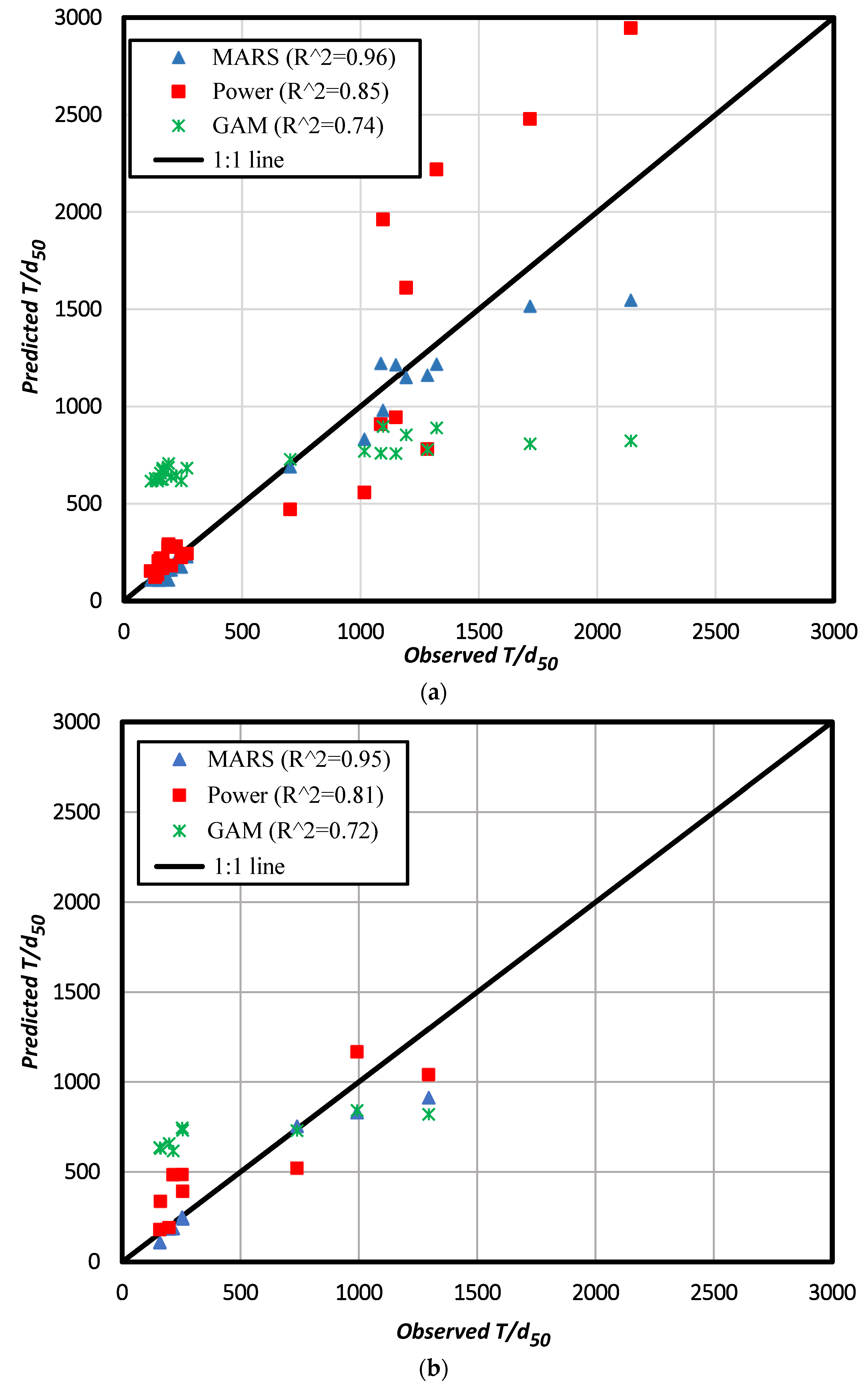
4.1. Comparison of the Models

Power, GAM, and MARS models were used to develop the relation for predicting $\frac{T}{d_{50}}$ versus the effective variables. To determine which model has the maximum adaptation with the observed data, the scatter graph was plotted for the training and testing data separately (Figure 4). Consequently, the MARS method matched the observed data better than the others, with the highest correlation coefficient of R² equal to 0.95 compared to power (0.81) and GAM (0.72). Also, the performance of the three developed models based on RMSE and MAE was calculated for both the training and testing data sets. In addition, the Mean Absolute Percentage Error, MAPE, was used from the following expression [46], to ensure that more accurate results were gained (

Table 6. Error analysis of predicted $\frac{T}{d_{50}}$ by power model against GAM and MARS.

	Training			Testing
Index	MARS	Power	GAM	MARS	Power	GAM
R2	0.96	0.85	0.74	0.95	0.81	0.72
RMSE	140.64	287.65	523.06	140.47	320.99	382.49
MAE	79.12	197.53	472.59	84.80	247.61	367.57
MAPE (%)	14.39	31.13	188.93	13.75	44.10	143.79

),

$$MAPE=\frac{1}{n}{\sum }_{i=1}^n\left|\frac{O_i-P_i}{O_i}\right|\times 100$$

(13)

where $O_i$and $P_i$ is related to both the real and predicted values for ith observation, respectively, and $n$ is the number of observations.

According to Table 6, all the error indicator values for MARS are less than the power and GAM models in both data sets. The value of RMSE was equal to 140.47 for MARS versus 320.99 and 382.49 for the two others in the testing data. In addition, the MAPE value of 13.75% was gained for the MARS in the testing situation. So, this model can present an adequate relation for predicting sediment particle size in the river bends with better results than the others. After the MARS, the power model gives proper outputs, indicating the ability of this traditional method to develop an empirical relation for sediment grain size determination.

Also, the performance of the three developed models based on RMSE and MAE was calculated for both the training and testing data sets. In addition, the mean absolute percentage error, MAPE, ref. [46], was applied to ensure that more accurate results were gained (Table 6).

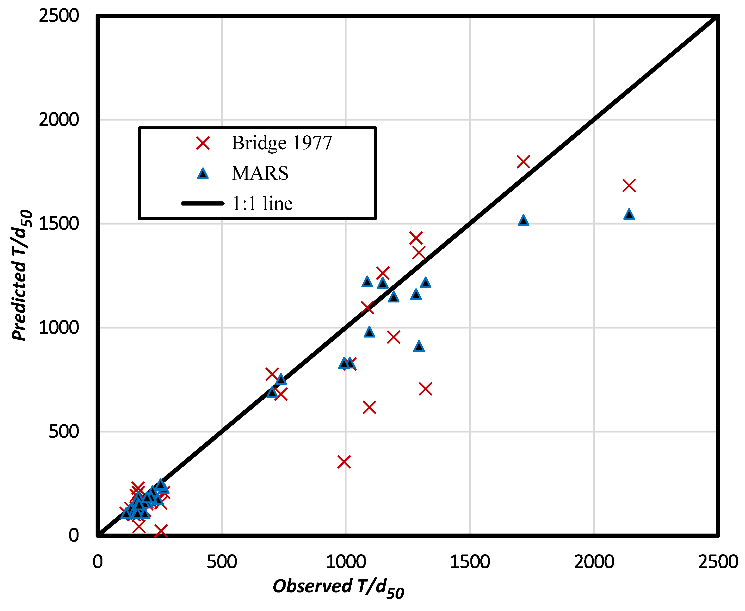
4.2. Comparison of MARS with Analytical Method

To validate the superior model (MARS) with an analytical approach, Bridge’s relation [5] was used. This relation calculates the median size of bed sediments in river bends for steady nonuniform flow and noncircular (sine-generated) bend conditions (Equation (14)).

$$D=\frac{3{\tau }_b}{2\left({\rho }_s-{\rho }_w\right)g(\cos \alpha \tan \phi \cos \gamma -\sin \gamma )}$$

(14)

where $D$ is the median size of bed sediments, $\alpha$ and $\gamma$ are the bed transverse and longitudinal slopes, $\phi$ shows the angle of internal friction, and other parameters have already been introduced.

The values of $d_{50}$ calculated by Bridges’ relation utilizing the field data were used to obtain $T/d_{50}$ in the bends. Then, both analytical and MARS models’ results were compared with the observed data, as shown in Figure 5. The MARS results presented a better fit than the analytical method with a higher R², which equals 0.96 against 0.89.

Furthermore, the outputs of the RMSE, MAE, and MAPE indices showed that the MARS performed better than the Bridge’s relation (

Table 7. Error analysis of predicted $\frac{T}{d_{50}}$ by MARS against the analytical model.

Index	MARS	Analytical Model
R2	0.96	0.89
RMSE	140.64	200.21
MAE	78.78	116.44
MAPE (%)	14.22	23.46

).

The error percentage (MAPE) of the MARS model (14.22%) is about 9 percent less than the value of the analytical model (23.46%).

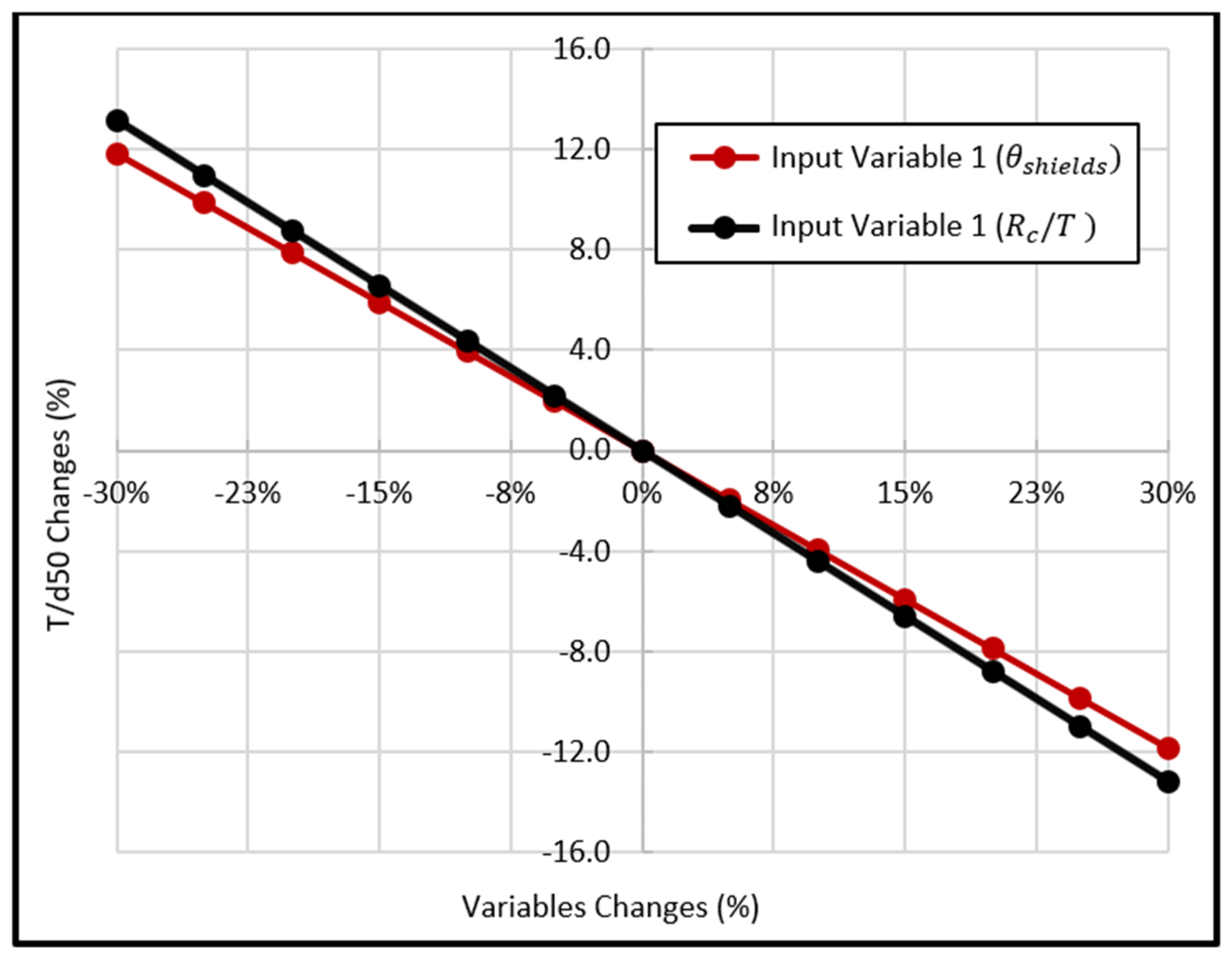
4.3. Sensitivity and Uncertainty Analysis for MARS Model

The sensitivity analysis for input parameters in the proposed MARS model was performed. Two parameters, ${\theta }_{shields}$ and $\frac{R_c}{T}$, affected the model’s output. Figure 6 shows the changes in the percentage of $\frac{T}{d_{50}}$ against the variable’s change percentage.

The figure shows that with a change of 5% to 30% of the values of ${\theta }_{shields}$ and $R_c/T$, $T/d_{50}$ will change about 3.5% to 18% and 2% to 13%, respectively. This represents the sensitivity of the MARS model results to the input variables within the uncertainty in the model. Also, analysis of the uncertainty of the MARS along with the power, GAM, and analytical method for prediction of the bend of gravel-bed rivers is demonstrated in

Table 8. Uncertainty analysis for the prediction of $\frac{T}{d_{50}}$ by MARS and other approaches.

Model	Mean Prediction Error	Width of Confidence Band	95% Confidence Interval of Mean Prediction Error
MARS	−63.27	$\pm$42.22	−105.49–21.05
Analytical model	−90.09	$\pm$62.43	−152.52–27.66
Power	91.71	$\pm$108.00	−16.29–199.71
GAM	145.76	$\pm$159.75	−13.99–305.51

. This table reflects the mean prediction errors, the width of the confidence band, and the 95% confidence interval of the mean prediction errors. The mean prediction error was calculated based on the average error for each data set; the width of the confidence band was determined via the error and Standard Deviation (SD) according to the Wilson score method; and the 95% confidence interval of the mean prediction errors can be specified as $\pm 1.96$SD [28,47].

The values of the mean prediction error and the minimum confidence band width for MARS are −63.27 and $\pm$42.22, respectively. These demonstrate that the MARS is more suitable for the prediction of $T/d_{50}$ than the other methods.

5. Conclusions

This study has developed an empirical relation capable of estimating the median sediment particle size ($d_{50}$) in gravel river bends. Field data were collected from different cross-sections placed at bend apex and crossovers in various rivers. By using these data and dimensional analysis procedures, $\frac{T}{d_{50}}$ was calculated at the bends’ cross-sections. Applying correlation analysis between variables showed that the cross-sectional mean flow velocity, $\overline{u}$, bed shear stress, ${\tau }_b$, radius curvature, $R_c$, as well as sediment density, ${\rho }_s$, were essential parameters to generate the nondimensional variables containing Froude number, $Fr$, Shields parameter, ${\theta }_{shields}$, the curvature ratio, $\frac{R_c}{T}$, and the submerged weight of sediment, $(SG-1)$, respectively. These parameters based on the collected field data were restricted to $Fr$ < 1, 0.01 ≤ ${\theta }_{shields}$ ≤ 0.11, 2.62 ≤ $\frac{R_c}{T}$ ≤ 19.18, and 1.65 ≤ $SG-1$ ≤ 1.74. In the following, we applied three regression models (power, GAM, and MARS) to develop an appropriate relation between the geometric, hydraulic, and sedimentary parameters. Then, statistical metrics were employed to compare and choose the best-fitted model. Finally, MARS, as the preferred one, was validated with the analytical model, and sensitivity and uncertainty analyses were performed for it. It seems that the relation developed here has enough robustness to predict the bed sediment size in river bends. Other conclusions have been established from this research, as considered below:

• It was found that two parameters, $R_c/T$ and ${\theta }_{shields}$, are the most important in affecting $d_{50}$. This means that ${\tau }_b$ and $R_c$ from the flow hydraulic and channel geometry characteristics are the significant parameters to determine $d_{50}$ in meandering river bends.
• The MARS formula showed that it was a better match with the observed data than power and GAM and had less error compared with the analytical model of Bridge. Although this needs to be assessed in more rivers, it can be an appropriate relation to calculate $d_{50}$ in gravel channel bends in engineering applications within parameter ranges.
• There have been rare studies to determine the sediment particle sizes in river bends, and the existing relations, such as Bridge’s model, do not provide physical insight on how bend parameters affect sediment size. The proposed relation in this current article provides a reliable evaluation of sediment sizes based on bend characteristics.
• After MARS, the power model created better outputs. Even if this is a traditional approach, it presents a simpler relation with fairly good results for determining the size of sediment particles in bends.

References

1. Rovira, A.; Núñez-González, F.; Ibañez, C. Dependence of Sediment Sorting on Bedload Transport Phase in a River Meander. Earth Surf. Process. Landf. 2018, 43, 2077–2088. [Google Scholar] [CrossRef]
2. Cordier, F.; Tassi, P.; Claude, N.; Crosato, A.; Rodrigues, S.; Pham Van Bang, D. Bar Pattern and Sediment Sorting in a Channel Contraction/Expansion Area: Application to the Loire River at Bréhémont (France). Adv. Water Resour. 2020, 140, 103580. [Google Scholar] [CrossRef]
3. Fernández, R.; Vitale, A.J.; Parker, G.; García, M.H. Hydraulic Resistance in Mixed Bedrock-Alluvial Meandering Channels. J. Hydraul. Res. 2021, 59, 298–313. [Google Scholar] [CrossRef]
4. Li, J.; He, X.; Wei, J.; Bao, Y.; Tang, Q.; de Nambajimana, J.D.; Nsabimana, G.; Khurram, D. Multifractal Features of the Particle-Size Distribution of Suspended Sediment in the Three Gorges Reservoir, China. Int. J. Sediment Res. 2021, 36, 489–500. [Google Scholar] [CrossRef]
5. Bridge, J.S. Flow, Bed Topography, Grain Size and Sedimentary Structure in Open Channel Bends: A Three-Dimensional Model. Earth Surf Process. 1977, 2, 401–416. [Google Scholar] [CrossRef]
6. Odgaard, A.J. Grain Size Distribution of River Bed Armor Layers. J. Hydraul. Eng. 1984, 110, 1479–1484. [Google Scholar] [CrossRef]
7. Milhous, R.T. Effect of Sediment Transport and Flow Regulation on the Ecology of Gravel-Bed Rivers; John Wiley & Sons: Chichester, UK, 1982; pp. 819–842. [Google Scholar]
8. Julien, P.Y.; Anthony, D.J. Bed Load Motion and Grain Sorting in a Meandering Stream. J. Hydraul. Res. 2002, 40, 125–133. [Google Scholar] [CrossRef]
9. Wright, S.; Parker, G. Modeling Downstream Fining in Sand-Bed Rivers. I: Formulation. J. Hydraul. Res. 2010, 43, 613–620. [Google Scholar] [CrossRef]
10. Jang, J.-H.; Ho, H.; Yen, C. Effects of Lifting Force on Bed Topography and Bed-Surface Sediment Size in Channel Bend. J. Hydraul. Eng. 2011, 137, 911–920. [Google Scholar] [CrossRef]
11. Kuhnle, R.A.; Wren, D.G.; Langendoen, E.J. Structural Changes of Mobile Gravel Bed Surface for Increasing Flow Intensity. J. Hydraul. Eng. 2019, 146, 04019065. [Google Scholar] [CrossRef]
12. McKie, C.W.; Juez, C.; Plumb, B.D.; Annable, W.K.; Franca, M.J. How Large Immobile Sediments in Gravel Bed Rivers Impact Sediment Transport and Bed Morphology. J. Hydraul. Eng. 2021, 147, 04020096. [Google Scholar] [CrossRef]
13. White, D.C.; Nelson, P.A. Flume Investigation Into Mechanisms Responsible for Particle Sorting in Gravel-Bed Meandering Channels. J. Geophys. Res. Earth Surf. 2023, 128, e2022JF006821. [Google Scholar] [CrossRef]
14. Yen, C.; Lee, K.T. Bed Topography and Sediment Sorting in Channel Bend with Unsteady Flow. J. Hydraul. Eng. 1995, 121, 591–599. [Google Scholar] [CrossRef]
15. Pitlick, J.; Mueller, E.R.; Segura, C.; Cress, R.; Torizzo, M. Relation between Flow, Surface-Layer Armoring and Sediment Transport in Gravel-Bed Rivers. Earth Surf. Process. Landf. 2008, 33, 1192–1209. [Google Scholar] [CrossRef]
16. Naito, K.; Ma, H.; Nittrouer, J.A.; Zhang, Y.; Wu, B.; Wang, Y.; Fu, X.; Parker, G. Extended Engelund–Hansen Type Sediment Transport Relation for Mixtures Based on the Sand-Silt-Bed Lower Yellow River, China. J. Hydraul. Res. 2019, 57, 770–785. [Google Scholar] [CrossRef]
17. Bateni, S.M.; Vosoughifar, H.R.; Truce, B.; Jeng, D.S. Estimation of Clear-Water Local Scour at Pile Groups Using Genetic Expression Programming and Multivariate Adaptive Regression Splines. J. Waterw. Port Coast. Ocean. Eng. 2019, 145, 04018029. [Google Scholar] [CrossRef]
18. Bazrkar, M.H.; Chu, X. Development of Category-Based Scoring Support Vector Regression (CBS-SVR) for Drought Prediction. J. Hydroinform. 2022, 24, 202–222. [Google Scholar] [CrossRef]
19. Rajesh, M.; Rehana, S. Prediction of River Water Temperature Using Machine Learning Algorithms: A Tropical River System of India. J. Hydroinform. 2021, 23, 605–626. [Google Scholar] [CrossRef]
20. Abbasi, M.; Farokhnia, A.; Bahreinimotlagh, M.; Roozbahani, R. A Hybrid of Random Forest and Deep Auto-Encoder with Support Vector Regression Methods for Accuracy Improvement and Uncertainty Reduction of Long-Term Streamflow Prediction. J. Hydrol. 2021, 597, 125717. [Google Scholar] [CrossRef]
21. Park, S.; Hamm, S.Y.; Jeon, H.T.; Kim, J. Evaluation of Logistic Regression and Multivariate Adaptive Regression Spline Models for Groundwater Potential Mapping Using R and GIS. Sustainability 2017, 9, 1157. [Google Scholar] [CrossRef]
22. Asquith, W.H. Regression Models of Discharge and Mean Velocity Associated with Near-Median Streamflow Conditions in Texas: Utility of the U.S. Geological Survey Discharge Measurement Database. J. Hydrol. Eng. 2013, 19, 108–122. [Google Scholar] [CrossRef]
23. Asquith, W.H.; Herrmann, G.R.; Cleveland, T.G. Generalized Additive Regression Models of Discharge and Mean Velocity Associated with Direct-Runoff Conditions in Texas: Utility of the U.S. Geological Survey Discharge Measurement Database. J. Hydrol. Eng. 2013, 18, 1331–1348. [Google Scholar] [CrossRef]
24. Adnan, R.M.; Parmar, K.S.; Heddam, S.; Shahid, S.; Kisi, O. Suspended Sediment Modeling Using a Heuristic Regression Method Hybridized with Kmeans Clustering. Sustainability 2021, 13, 4648. [Google Scholar] [CrossRef]
25. Faraway, J.J. Extending the Linear Model with R: Generalized Linear, Mixed Effects and Nonparametric Regression Models, 2nd ed.; Chapman and Hall/CRC: Boca Raton, FL, USA, 2016; pp. 1–395. [Google Scholar] [CrossRef]
26. Hagemann, M.; Kim, D.; Park, M.H. Estimating Nutrient and Organic Carbon Loads to Water-Supply Reservoir Using Semiparametric Models. J. Environ. Eng. 2016, 142, 04016036. [Google Scholar] [CrossRef]
27. Mehdizadeh, S.; Behmanesh, J.; Khalili, K. Using MARS, SVM, GEP and Empirical Equations for Estimation of Monthly Mean Reference Evapotranspiration. Comput. Electron. Agric. 2017, 139, 103–114. [Google Scholar] [CrossRef]
28. Mohanta, A.; Patra, K.C. MARS for Prediction of Shear Force and Discharge in Two-Stage Meandering Channel. J. Irrig. Drain. Eng. 2019, 145, 04019016. [Google Scholar] [CrossRef]
29. Ihaka, R.; Gentleman, R. R: A Language for Data Analysis and Graphics. J. Comput. Graph. Stat. 1996, 5, 299. [Google Scholar] [CrossRef]
30. Germaine, J.T.; Germaine, A.V. Geotechnical Laboratory Measurements for Engineers; John Wiley & Sons: Hoboken, NJ, USA, 2009; pp. 1–351. [Google Scholar] [CrossRef]
31. Buckingham, E. On Physically Similar Systems; Illustrations of the Use of Dimensional Equations. Phys. Rev. 1914, 4, 345. [Google Scholar] [CrossRef]
32. Ferreira da Silva, A.M.; Ebrahimi, M. Meandering Morphodynamics: Insights from Laboratory and Numerical Experiments and Beyond. J. Hydraul. Eng. 2017, 143, 03117005. [Google Scholar] [CrossRef]
33. Ferreira da Silva, A.M.; Ana, M. Fluvial Processes (IAHR Monograph), 2nd ed.; CRC Press: Leiden, The Netherlands, 2017; pp. 1–289. [Google Scholar] [CrossRef]
34. Bartlett, M.S. Properties of Sufficiency and Statistical Tests. Proc. R. Soc. London. Ser. A Math. Phys. Sci. 1937, 160, 268–282. [Google Scholar] [CrossRef]
35. Froehlich, D.C. Neural Network Prediction of Maximum Scour in Bends of Sand-Bed Rivers. J. Hydraul. Eng. 2020, 146, 04020065. [Google Scholar] [CrossRef]
36. McCuen, R.H.; Leahy, R.B.; Johnson, P.A. Problems with Logarithmic Transformations in Regression. J. Hydraul. Eng. 1990, 116, 414–428. [Google Scholar] [CrossRef]
37. Najafzadeh, M.; Oliveto, G. Riprap Incipient Motion for Overtopping Flows with Machine Learning Models. J. Hydroinform. 2020, 22, 749–767. [Google Scholar] [CrossRef]
38. Finch, W.H. Multivariate Analysis of Variance for Multilevel Data: A Simulation Study Comparing Methods. J. Exp. Educ. 2022, 90, 173–190. [Google Scholar] [CrossRef]
39. Hastie, T.; Tibshirani, R. Generalized Additive Models, 1st ed.; ChapMan & Hall: Boca Raton, FL, USA, 1990; pp. 1–335. [Google Scholar]
40. Nejat Dehkordi, A.; Sharafati, A.; Mehraein, M.; Hoseini, S.A. Modelling of Sediment Grains Size Distribution in River Bend Using Generalized Additive Model. Water Irrig. Manag. 2022, 11, 713–724. [Google Scholar] [CrossRef]
41. Leathwick, J.R.; Elith, J.; Hastie, T. Comparative Performance of Generalized Additive Models and Multivariate Adaptive Regression Splines for Statistical Modelling of Species Distributions. Ecol. Modell. 2006, 199, 188–196. [Google Scholar] [CrossRef]
42. Witten, I.H.; Frank, E.; Hall, M.A. Data Transformations. In Data Mining: Practical Machine Learning Tools and Techniques; Morgan Kaufmann: Burlington, MA, USA, 2011; pp. 305–349. [Google Scholar] [CrossRef]
43. Moisen, G.G.; Frescino, T.S. Comparing Five Modelling Techniques for Predicting Forest Characteristics. Ecol. Model. 2002, 157, 209–225. [Google Scholar] [CrossRef]
44. Catalano, G.A.; D’Urso, P.R.; Maci, F.; Arcidiacono, C. Influence of Parameters in SDM Application on Citrus Presence in Mediterranean Area. Sustainability 2023, 15, 7656. [Google Scholar] [CrossRef]
45. Kuhn, M.; Johnson, K. Applied Predictive Modeling, 1st ed.; Springer Science & Business Media: New York, NY, USA, 2013; pp. 1–595. [Google Scholar] [CrossRef]
46. Amininia, K.; Saghebian, S.M. Uncertainty Analysis of Monthly River Flow Modeling in Consecutive Hydrometric Stations Using Integrated Data-Driven Models. J. Hydroinform. 2021, 23, 897–913. [Google Scholar] [CrossRef]
47. Sattar, A.M.A. Gene Expression Models for the Prediction of Longitudinal Dispersion Coefficients in Transitional and Turbulent Pipe Flow. J. Pipeline Syst. Eng. Pract. 2013, 5, 04013011. [Google Scholar] [CrossRef]
Figure 1. The location of the study areas in Zayandehrood, Karun, Khersan, and Niakan Rivers, Iran.
Water 16 00444 g001
Figure 2. Primary function forms to obtain the most appropriate model for each auxiliary variable in the GAM model: (a) T / d 50 versus S G 1 ; (b) T / d 50   versus F r .
Water 16 00444 g002
Figure 3. Primary function forms to obtain the most appropriate model for each auxiliary variable in the GAM model: (a) T / d 50 versus θ s h i e l d s ; (b) T / d 50 versus R c / T .
Water 16 00444 g003
Figure 4. Predicted T / d 50 versus observed with R2 for training and testing data: (a) Training data, n = 26; (b) Testing data, n = 9.
Water 16 00444 g004
Figure 5. MARS and Bridge results against observed values of T / d 50 for all the data, n = 35.
Water 16 00444 g005
Figure 6. Changes percentages of T / d 50 against θ s h i e l d s and R c / T change percentage.
Water 16 00444 g006