Predicting the Flow Fields in Meandering Rivers with a Deep Super-Resolution Convolutional Neural Network

Abstract

The hydrodynamic model, based on the strict conservation of momentum and continuity equations, can accurately simulate the distribution of a flow field. However, significant computing time and storage space requirements limit real-time prediction. Machine learning is well known for its fast computing speed and powerful learning ability, but its accuracy depends on an abundance of training data, hindering its wider use in locations without sufficient measurements. Application restrictions in data-deficient areas can be addressed through transfer learning, provided that two areas share common characteristics. In this study, a machine learning method based on a deep super-resolution convolutional neural network (DSRCNN) and transfer learning is proposed, validated, and applied to model two bend flows and one realistic test case. Firstly, the hydrodynamic model was established and validated against measured data. The validated model was considered to have the ability to generate real data and was used to generate a comprehensive data set for training and validating the machine learning model. Three different methods were compared and tested, with Realizable k-ε performing better than the others in predicting the outer bank flow distribution. DSRCNN was compared to a plain SRCNN (PSRCNN), as well as Bilinear, Nearest, and Bicubic methods, and the results showed that DSRCNN had the best performance. We compared Raw, RT, and TL methods, finding that the TL method performed the best overall. Therefore, the research results showed that the developed super-resolution convolutional neural network can provide more reliable predications and serve as an ideal tool for simulating flow field distribution in bends.

1. Introduction

The temporal and spatial distribution of river flow has both positive and negative effects on human beings. Studying the characteristics of the temporal and spatial distribution of river flow can help us reduce disadvantages, such as flooding or riverbed scouring, and potentially transform them into advantages for effective utilization [1,2,3]. The curved streamway is one of the most common waterway patterns in nature, and even straight rivers will transition to curved under the influence of various special factors in the natural environment [4]. The plane shape of a natural stable bend of a river is similar to a sine curve. Under the constraint of boundaries, the flow is simultaneously affected by non-uniform centripetal forces, wall shear stress, and pressure gradients generated by water surface gradients, which cause the flow field to be redistributed and form a complex three-dimensional spiral flow. This complex flow structure leads to sediment movement, riverbed evolution, channel deformation, etc. [5]. Therefore, the study of bend flow is significant.

River flow characteristics have been investigated by numerous researchers using physical experimental approaches. For instance, Shen and Haas [6] conducted a 3D model experiment to calculate river age. Jun et al. [7] studied the phenomenon and mechanism of ice accretion in a curved channel under different flow and ice flow conditions. Huang [8] carried out a physical simulation study on the height, propagation velocity, tidal current velocity, front gradient, and bore shape of a tidal bore in a rectangular flume. Zhang et al. [9] performed an experimental study on the sediment transport and changes in riverbed morphology caused by the asymmetric confluence of tributaries in the upper Yellow River. Van Dael et al. [10] utilized an experimental flume to examine the effect of water flow velocity and sediment Fe/P ratio. Stelzer et al. [11] employed the scaled physical model to simulate riverbed sedimentation in its natural state. As an integral part of nature, water flow exhibits diverse hydraulic characteristics under the influence of various natural factors [12]. The regularity of water characteristics can be determined through model experiments and extrapolated into the actual production environment using various specialized methods [13]. However, physical experiments are subject to numerous uncontrollable factors, impacting accuracy and requiring additional time, manpower, and material resources for experiment replication. Hence, alternative methods that can mitigate these disadvantages are necessary.

With the continuous advancement of computer storage, calculation, and programming, and the measurement of hydraulic and hydrological data [14], it has become feasible to employ numerical simulation technology for studying physical and mechanical properties of water characteristics. For example, Chang et al. [15] investigated the freezing process of water droplets on different hydrophobic surfaces through experiments and simulations. Patsinghasanee et al. [16] carried out an experimental and numerical study on the impact of a tidal bore on a sheet pile spur dike at Qiantang River. Mouri et al. [17] explored the characteristics of a sand-retaining dam affecting sediment regulation function in the river. Cai et al. [18] investigated tidal impact by integrating a flume experiment with software prediction. In recent years, hydrodynamic numerical models have been widely employed to study hydrodynamic characteristics. These models can be categorized into 1D, 2D, and 3D, with extensive research and progress made in addressing 2D and 3D problems [19]. However, the calculation accuracy of a 2D hydraulic model is not as high as that of a 3D hydraulic model [20]. The significant computational time and storage space required make the 3D numerical model calculations expensive [12], and the prediction lag restricts its ability to provide real-time results for hydraulic elements during disasters. These factors impose limitations on the utilization of 3D hydraulic numerical models.

Machine learning can serve as a supplementary to address the problem of expensive calculation [21]. This method has been applied in many fields [22,23,24,25,26], and has shown that these methods, such as convolutional neural networks, are effective tools to generate 3D flow field elements [27]. In addition, machine learning can adaptively compute implicit relationships through a certain amount of input and the numerical value [28], reducing the impact of various factors assumed artificially in advance, and improve the accuracy of the model [29]. However, the improvement of this accuracy relies on having sufficient data [30]. This dependency makes it impossible to use this method for rivers with insufficient data [12]. The amount of available data is often related to the development of a river, and a river with insufficient development may contain great value with respect to potential power and water resources [31].

To solve the above-mentioned problems, this article proposes a super-resolution deep learning method, using the ground truth data generated by OpenFOAM and Telemac, and evaluates its applicability and effectiveness. This research was carried out under the current lack of efficient and accurate numerical simulation results. The developed AI model can carry out super-resolution processing and obtain the data research content of this research area based on a small number of observation point data. In this study, the developed model was compared with the traditional model, and the results were found to be superior for the developed model. To further prove the practical applicability, the Xiaosi River was simulated using hydrodynamic software, and a comprehensive data set was obtained through numerical simulation experiments. Finally, the whole method framework was combined and applied to a real river case using transfer learning to simulate the flow field distribution in the actual environment. The performance of the Xiaosi River via the transfer learning method showed a good simulation result.

The structure of this paper is as follows. Section 2 introduces the research area, the governing equations of the numerical model, and the performance metrics of the model. Section 3 introduces the simulation performance. Section 4 discusses the applicability and limitations of transfer learning, and the findings are summarized in Section 5.

2. Methodology

2.1. Overall Research Strategy

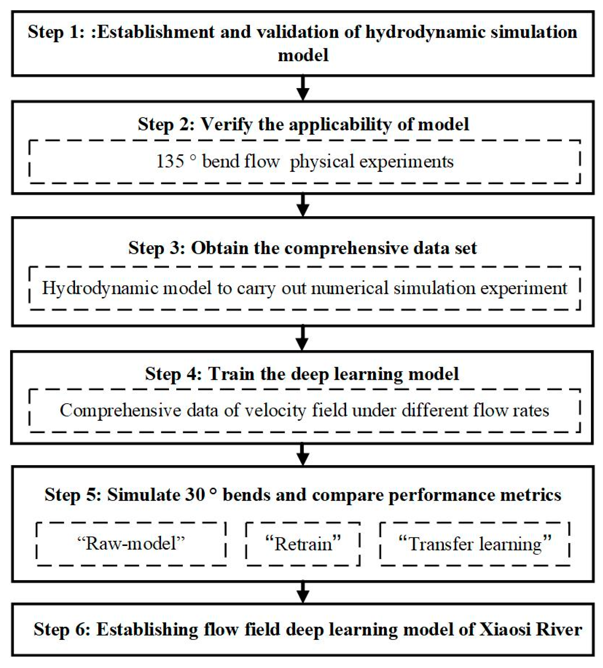
Figure 1 presents the overall flow chart of the study, which illustrates the detailed process of algorithm establishment and verification. The relevant operational steps involved in this study are listed as follows:

Step 1: Establish the hydrodynamic model;

Step 2: Carry out the physical experiments under 135° bend flow and verify the applicability of the model;

Step 3: Carry out numerical simulation experiments to obtain the comprehensive data set of flow velocity field in a 135° bend with different flow rates;

Step 4: Use the comprehensive data set of the velocity field to train the deep learning model;

Step 5: Use three different super-resolution methods to model 30° bends and compare performance metrics;

Step 6: Establish a flow field deep learning model of the Xiaosi River.

Figure 1. The detailed process of algorithm establishment and verification.

Figure 1. The detailed process of algorithm establishment and verification.

In the following content, we will introduce the implementation methods of laboratory experience in Section 2.2, realistic case and fieldwork in Section 2.3, and numerical models in Section 2.4 (including Delft3D and OpenFOAM). Section 2.5 will cover datasets and data processing, while Section 2.6 will introduce machine learning methods. Lastly, Section 2.7 will cover performance metrics.

2.2. Laboratory Experiment

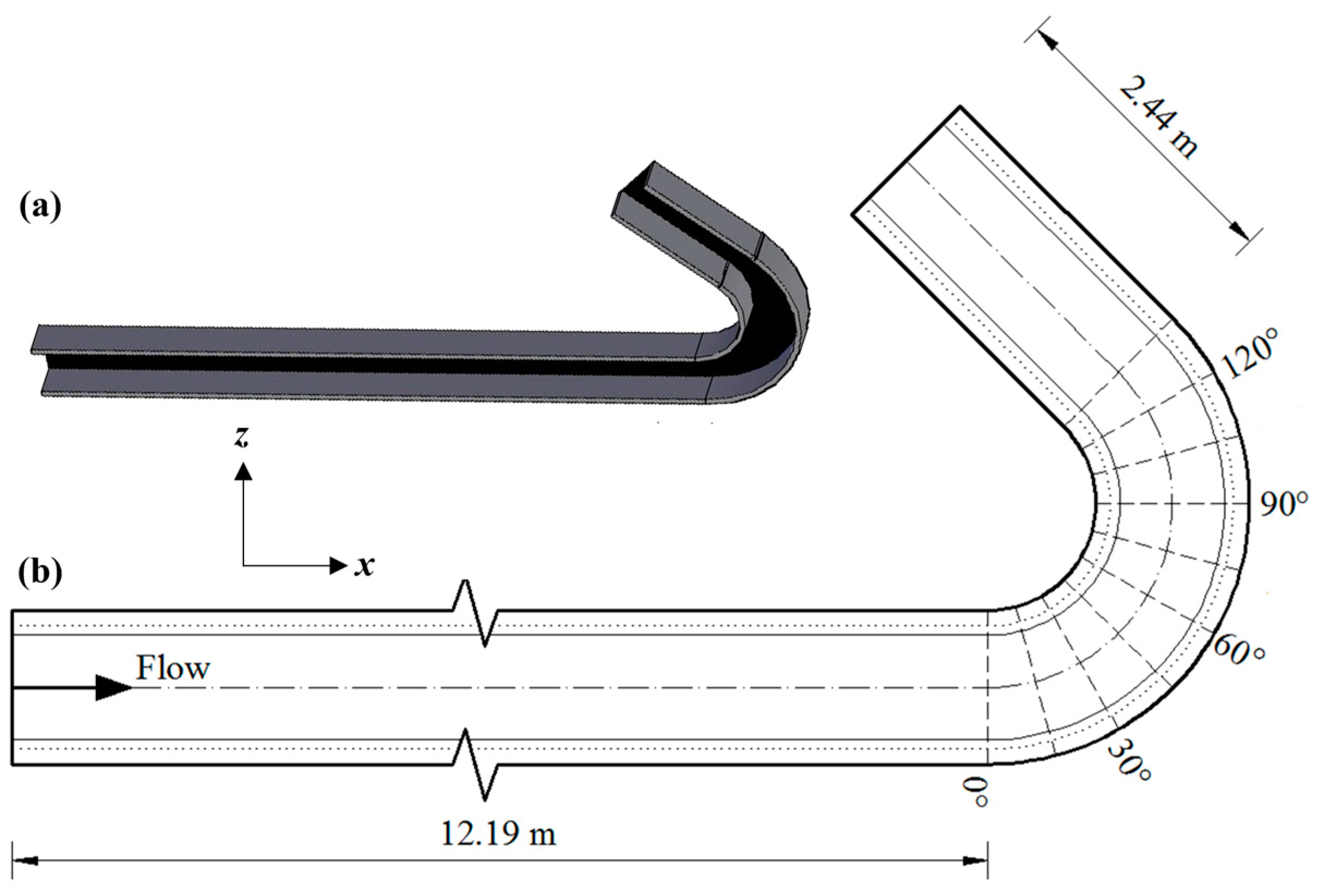
Figure 2 shows the 135° bend used in this case. The channel consists of two straight channels connected by 135° bends. The straight pipe at the inlet section is 12.19 m long, and the straight pipe at the outlet section is 2.44 m long [32]. The curvature ratio (Rc/b) is 1.5. The cross section of the channel is a rectangle with a length of 1 m and a width of 0.9 m. The material of the side wall is high vertical acrylic plate. A layer of quartz sand (with a median grain diameter of 0.689 × 10⁻³ m) was laid on the ground and hardened with Plaster of Paris and spar urethane to simulate the sedimentary riverbed. The water depth was controlled to be 0.15 m at 2 m upstream of the interface between the inlet straight pipe and the 135° elbow. In the experiment, two parameters, flow and flow velocity, were measured. The flow was measured at the 90° V-notch weir at the outlet section, and the accuracy of the results was verified through the ADV measurement of the straight pipe section at the inlet. The three-dimensional velocity was measured using Nortek Vectrino ADV at equidistant points along the pipeline, which were located 0.083 m, 0.250 m, 0.417 m, 0.584 m, 0.751 m, and 0.918 m away from the outer bank.The measuring point was 0.012 m to 0.092 m above the river bed, and the points were taken once every 0.01 m. The method of measuring flow parameters and the data processing process has been well documented elsewhere in the literature [33,34,35].

2.3. Realistic Case and Field Work

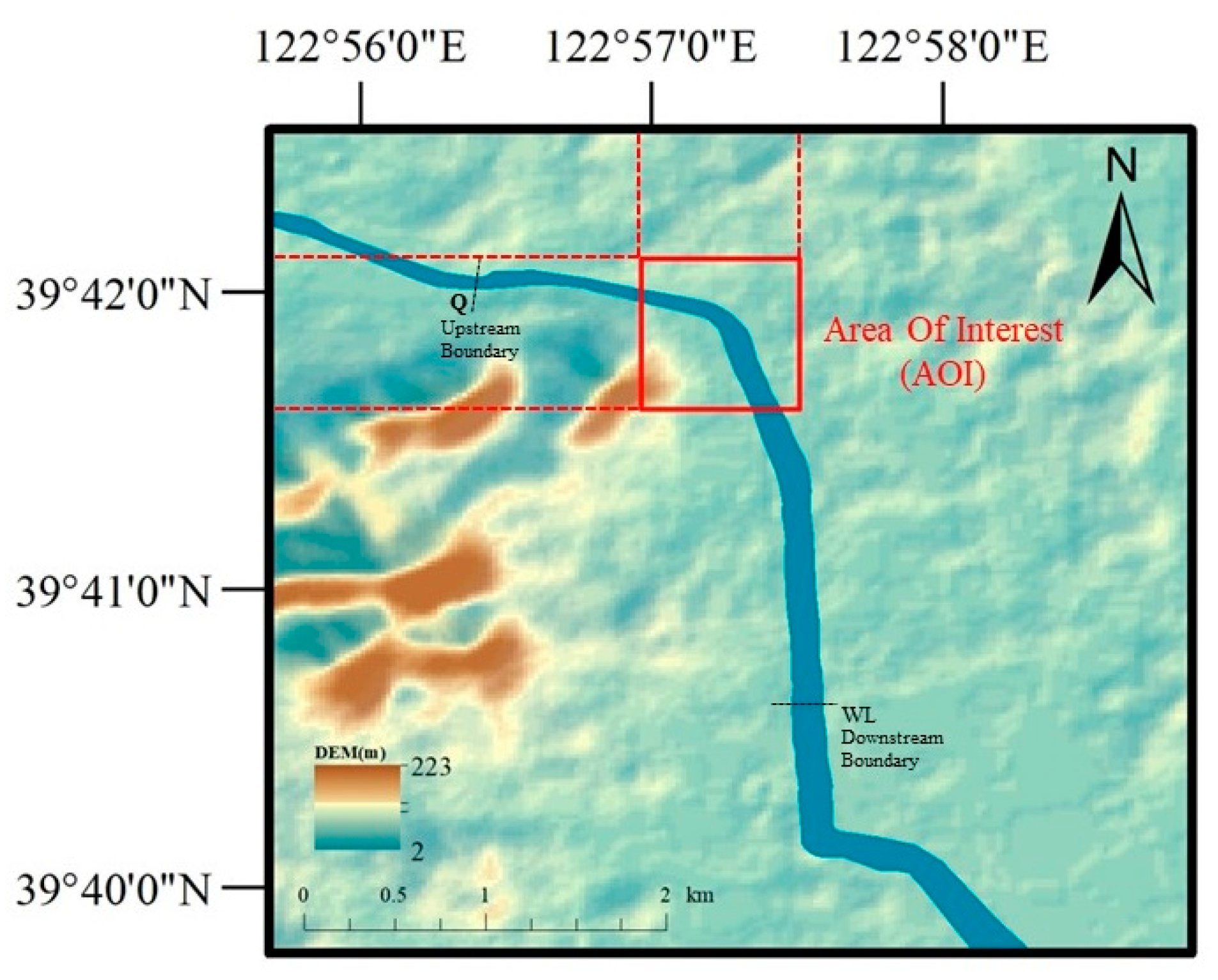
In this study, we selected a segment of the Xiaosi River as the study area, and obtained the required field data through a field survey. The Xiaosi River, which is located within the county boundary in Liaoning Province, is 32 km long with a drainage area of 241 km². Its location map can be seen in Figure 3. It is a natural drainage basin originating from Sanjiao Mountain, with an elevation of 87.9 m and an average river gradient of 1.27‰. Because it is a river course in Zhuanghe City, flooding there will cause great losses; thus, it is of great significance to quickly predict its water flow. The highly representative bend section upstream of the rubber dam of the Xiaosi River is selected as the research case. In this study, the two types of data required are elevation and velocity. The elevation data were provided by the relevant competent department, and the velocity data were measured by the research group using an LS300-A Portable Velocity Measuring Instrument. On 8 October 2022, a roughly zigzag route survey was carried out, and flow velocity and water depth data at 118 points were collected. The average value of velocity values at five different depths was taken as the depth averaged flow velocity. The upstream flow was 15.87 m³/s and the downstream water level was 4 m.

2.4. Numerical Models

OpenFOAM and Delft3D models were used for the numerical simulation (DELFT3D FM, OPENFOAM 2.3.1). The laboratory test case was based on OpenFOAM, the fluid model frame of the open source software platform for lab-wide three-dimensional high-precision numerical simulations. Delft3D, which better fits the real situation, was selected for simulation in the case study of the Xiaosi River. To some extent, OpenFOAM has been applied to various developments, such as the exploration of applicable environments and the improvement of application methods. Many studies have demonstrated the feasibility of OpenFOAM in flow structure velocity simulation [36,37,38].

The simulation conditions and schemes for OpenFOAM are introduced as follows:

Table 1. Method for discretizing different items.

Term	Scheme
Temporal term	Euler scheme
Gradient and Laplacian term	Gauss linear scheme
Divergence term	Combined Gauss linear, Gauss vanLeer, and Gauss upwind scheme
Pressure field	Preconditioned conjugate gradient (PCG) method, combined with a diagonal incomplete Cholesky (DIC) pre-conditioner, with a specified tolerance of 10−7

shows the methods we have selected for the discretization of different items. These selected algorithms demonstrated superior performance in numerical stability and accuracy compared to alternative methods. The linear method was chosen for interpolation schemes.

In the simulation process, a default time step interval of 0.01 s was initially chosen. This default value, however, was not rigid and allowed for dynamic adjustments based on a carefully defined numerical stability criterion. To maintain stability in the simulation, the maximum Courant number was set to 1. Sensitivity simulations were conducted to assess the impact of varying the default time step and Courant number. Remarkably, these analyses revealed that reducing these parameters did not lead to significant alterations in the simulation outcomes. The system achieved a state of near-steadiness after approximately 40 s of simulation time. However, to ensure a comprehensive understanding and account for any potential long-term trends or behaviors, all simulations were conservatively extended up to 120 s.

Delft3D, a unique, fully integrated computer software, has a multidimensional simulation program capable of computing non-steady flow. The main advantage over other hydrodynamic models is the ability to better simulate shallow water and sinuous complex boundaries and to generate orthogonal networks quickly. The calculation of the model was solved based on explicit and implicit alternating numerical integration in a finite difference method. It has high stability, fast calculation speed, and a flexible framework, which can obtain a better simulation effect, and can be transferred and used in software such as Arc GIS and MATLAB. Meanwhile, the flow module is able to build a straight or curvilinear grid of different scales to calculate the nonstable flow, and it provides rich open boundary conditions and initial conditions in the calculation. Delft3D has been widely used. For instance, Geng et al. [39] used Delft3D to simulate the spatial distribution of sediment particle size; Li et al. [40] used Delft3D to conduct a process-based modeling study to separate the effects of hydrological control on fracture morphology dynamics; and Lei et al. [41] applied the Delft3D model with PM to Shenzhen Bay, China, to verify the effectiveness of PM.

The simulation conditions and schemes for Delft3D are introduced as follows: the Conveyance-2D type utilizes R = HU, the Advection type employs Perot q(uio-u) fast, the advection velocity limiter type relies on monotone central, and the solver type is chosen as sobekGS + Saadilud.

2.4.1. Governing Equations for OpenFOAM

Three-dimensional Reynolds–averaged Navier–Stokes equations are the governing equations for three-digit high-precision simulations, which are the main methods for simulating complex viscous fields. The flow solution in the 3D region is mainly controlled using the continuity equation and momentum equation [42]:

The continuity equation is expressed as:

$$\frac{\mathtt{\partial }}{\mathtt{\partial }x}\left(u_x\right)+\frac{\mathtt{\partial }}{\mathtt{\partial }y}\left(u_y\right)+\frac{\mathtt{\partial }}{\mathtt{\partial }z}\left(u_z\right)=0$$

(1)

The momentum equation in the x-direction is expressed as:

$$\frac{\mathtt{\partial }\left(\rho u_x\right)}{\mathtt{\partial }t}+\frac{\mathtt{\partial }}{\mathtt{\partial }x}\left(\rho u_x{u}_x\right)+\frac{\mathtt{\partial }}{\mathtt{\partial }y}\left(\rho u_y{u}_x\right)+\frac{\mathtt{\partial }}{\mathtt{\partial }z}\left(\rho u_z{u}_x\right)=-\frac{\mathtt{\partial }p}{\mathtt{\partial }x}+\frac{\mathtt{\partial }{\tau }_{xx}}{\mathtt{\partial }x}+\frac{\mathtt{\partial }{\tau }_{yx}}{\mathtt{\partial }y}+\frac{\mathtt{\partial }{\tau }_{zx}}{\mathtt{\partial }z}+\rho g_x$$

(2)

The momentum equation in the y-direction is expressed as:

$$\frac{\mathtt{\partial }\left(\rho u_y\right)}{\mathtt{\partial }t}+\frac{\mathtt{\partial }}{\mathtt{\partial }x}\left(\rho u_x{u}_y\right)+\frac{\mathtt{\partial }}{\mathtt{\partial }y}\left(\rho u_y{u}_y\right)+\frac{\mathtt{\partial }}{\mathtt{\partial }z}\left(\rho u_z{u}_y\right)=-\frac{\mathtt{\partial }p}{\mathtt{\partial }y}+\frac{\mathtt{\partial }{\tau }_{xy}}{\mathtt{\partial }x}+\frac{\mathtt{\partial }{\tau }_{yy}}{\mathtt{\partial }y}+\frac{\mathtt{\partial }{\tau }_{zy}}{\mathtt{\partial }z}+\rho g_y$$

(3)

The momentum equation in the z-direction is expressed as:

$$\frac{\mathtt{\partial }\left(\rho u_z\right)}{\mathtt{\partial }t}+\frac{\mathtt{\partial }}{\mathtt{\partial }x}\left(\rho u_x{u}_z\right)+\frac{\mathtt{\partial }}{\mathtt{\partial }y}\left(\rho u_y{u}_z\right)+\frac{\mathtt{\partial }}{\mathtt{\partial }z}\left(\rho u_z{u}_z\right)=-\frac{\mathtt{\partial }p}{\mathtt{\partial }z}+\frac{\mathtt{\partial }{\tau }_{xz}}{\mathtt{\partial }x}+\frac{\mathtt{\partial }{\tau }_{yz}}{\mathtt{\partial }y}+\frac{\mathtt{\partial }{\tau }_{zz}}{\mathtt{\partial }z}+\rho g_z$$

(4)

where ρ = density; t = time; u_x, u_y, and u_z are velocity components; p = pressure; τ_ij = the force along the j direction on the i coordinate plane; and g_x, g_y, and g_z are gravitational acceleration components.

2.4.2. Governing Equations for Delft3D

The model is mainly controlled by the continuity equation and the momentum equation in the horizontal direction [43].

The continuity equation is expressed as:

$$\frac{\mathtt{\partial }\zeta }{\mathtt{\partial }t}+\frac{1}{\sqrt{G_{\xi \xi }}\sqrt{G_{\eta \eta }}}\frac{\mathtt{\partial }[(d+\zeta )U\sqrt{G_{\eta \eta }}]}{\mathtt{\partial }\xi }+\frac{1}{\sqrt{G_{\xi \xi }}\sqrt{G_{\eta \eta }}}\frac{\mathtt{\partial }[(d+\zeta )V\sqrt{G_{\xi \xi }}]}{\mathtt{\partial }\eta }=(d+\zeta )Q$$

(5)

$$U=\frac{1}{d+\zeta }{\displaystyle {\int }_d^{\zeta }u}dz={\displaystyle {\int }_{-1}^{0}u}d\sigma$$

(6)

$$V=\frac{1}{d+\zeta }{\displaystyle {\int }_c^{\zeta }v}dz={\displaystyle {\int }_{-1}^{0}v}d\sigma$$

(7)

$$Q={\displaystyle {\int }_{-1}^0(q_{in}-}{q}_{out})d\sigma +P-E$$

(8)

where U and V are depth average velocities; Q is water, precipitation and evaporation per unit area; q_in and q_out refer to the inflow and outflow of unit volume of water, respectively; P is non-local precipitation; and E is non-local evaporation.

The momentum equation in the ξ- and η-directions is expressed as:

$$\begin{array}{l}\frac{\mathtt{\partial }u}{\mathtt{\partial }t}+\frac{u}{\sqrt{G_{\xi \xi }}}\frac{\mathtt{\partial }u}{\mathtt{\partial }\xi }+\frac{v}{\sqrt{G_{\eta \eta }}}\frac{\mathtt{\partial }u}{\mathtt{\partial }\eta }+\frac{\varpi }{d+\zeta }\frac{\mathtt{\partial }u}{\mathtt{\partial }\sigma }-\frac{v^2}{\sqrt{G_{\xi \xi }}\sqrt{G_{\eta \eta }}}\frac{\mathtt{\partial }\sqrt{G_{\eta \eta }}}{\mathtt{\partial }\eta }+\frac{uv}{\sqrt{G_{\xi \xi }}\sqrt{G_{\eta \eta }}}\frac{\mathtt{\partial }\sqrt{G_{\xi \xi }}}{\mathtt{\partial }\eta }\\ -fv=-\frac{1}{{\rho }_0\sqrt{G_{\xi \xi }}}{P}_{\xi }+F_{\xi }+\frac{1}{{(d+\zeta )}^2}\frac{\mathtt{\partial }}{\mathtt{\partial }\sigma }(\nu v\frac{\mathtt{\partial }u}{\mathtt{\partial }\sigma })+M_{\xi }\end{array}$$

(9)

$$\begin{array}{l}\frac{\mathtt{\partial }v}{\mathtt{\partial }t}+\frac{u}{\sqrt{G_{\xi \xi }}}\frac{\mathtt{\partial }v}{\mathtt{\partial }\xi }+\frac{v}{\sqrt{G_{\eta \eta }}}\frac{\mathtt{\partial }v}{\mathtt{\partial }\eta }+\frac{\varpi }{d+\zeta }\frac{\mathtt{\partial }v}{\mathtt{\partial }\sigma }+\frac{uv}{\sqrt{G_{\xi \xi }}\sqrt{G_{\eta \eta }}}\frac{\mathtt{\partial }\sqrt{G_{\eta \eta }}}{\mathtt{\partial }\xi }-\frac{u^2}{\sqrt{G_{\xi \xi }}\sqrt{G_{\eta \eta }}}\frac{\mathtt{\partial }\sqrt{G_{\xi \xi }}}{\mathtt{\partial }\eta }\\ -fu=-\frac{1}{{\rho }_0\sqrt{G_{\eta \eta }}}{P}_{\eta }+F_{\eta }+\frac{1}{{(d+\zeta )}^2}\frac{\mathtt{\partial }}{\mathtt{\partial }\sigma }(\nu v\frac{\mathtt{\partial }v}{\mathtt{\partial }\sigma })+M_{\eta }\end{array}$$

(10)

The vertical eddy viscosity coefficient is defined by:

$$\nu v={\nu }_{mol}+\max ({\nu }_{3D},{\nu }^{back}v)$$

(11)

Density variations are neglected, except in the baroclinic pressure terms. P_ξ and P_η indicate the pressure gradient; the forces F_ξ and F_η indicate the imbalance of the horizontal Reynolds stress. M_ξ and M_η indicate the change caused by external momentum. ν_mol indicates the kinematic viscosity of water.

2.5. Datasets and Data Processing

Comprehensive data sets are needed for training and validating a model. In this study, three comprehensive data sets were established for a 135° bend, a 30° bend, and the Xiaosi River bend. The high-precision OpenFOAM was used to conduct the simulation study of the laboratory curve situation. Our group established 20 cases under different upstream flows for this method. Delft3D was used for the simulation of the Xiaosi River bend. This method only required 8 cases for training, and each case corresponded to an upstream flowrate condition. The model must prepare high-resolution data and low-resolution data. The high-resolution data were provided by the hydrodynamic model and extracted, using ParaView and MATLAB R2021a, from the outputs of the hydraulic models. We used ParaView to import simulation data into an Excel file and then utilized MATLAB to extract and process the data. MATLAB is more convenient for matrix processing as it does not require the import of additional packages by the authors. The low-resolution data were extracted using the decimate function of MATLAB, and the data scaling ratio was set to 8.

2.6. Machine Learning Methodology

2.6.1. Deep Super-Resolution Convolutional Neural Network

Super-resolution processing is used to estimate high-resolution images or video sequences based on low-resolution ones [44]. Deep learning algorithms build models for network analysis and learning to simulate the mechanism of the human brain to interpret data information. Super-resolution technology based on deep learning can improve image resolution under existing hardware conditions [45].

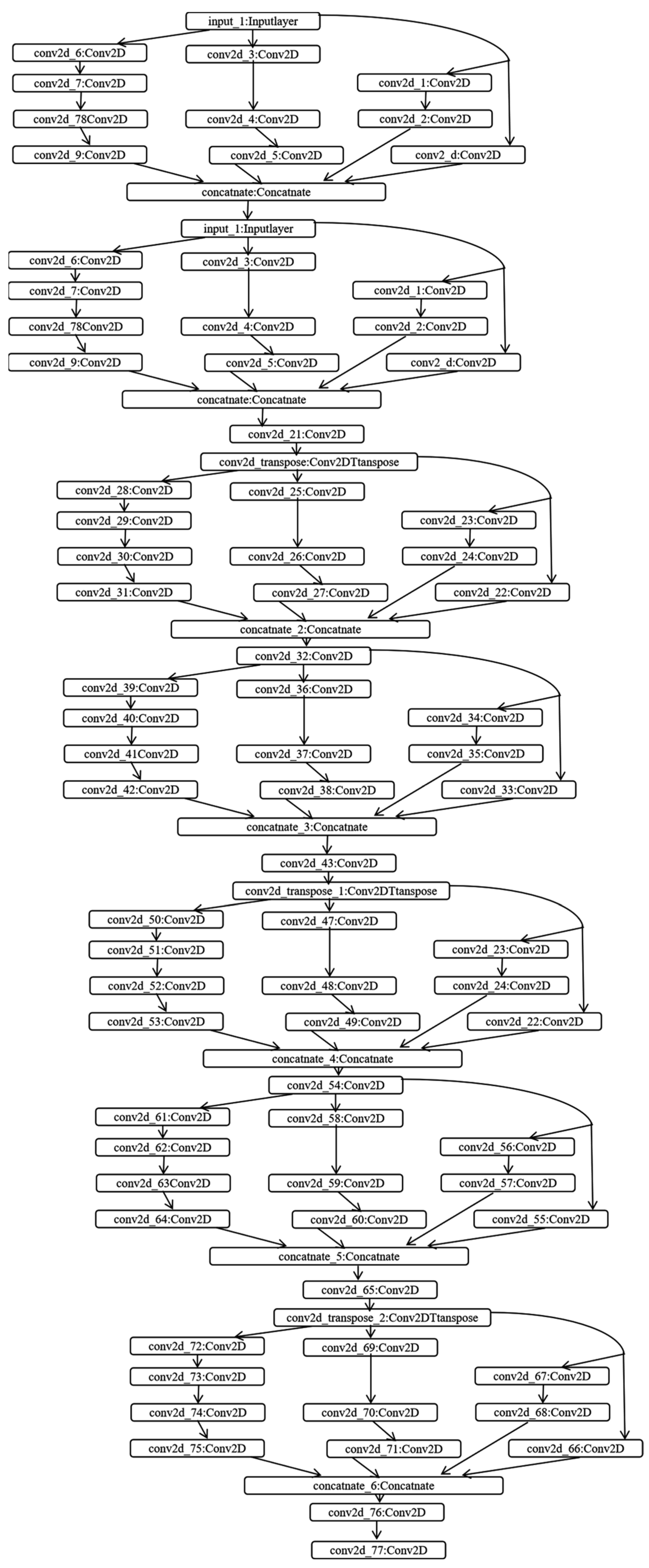
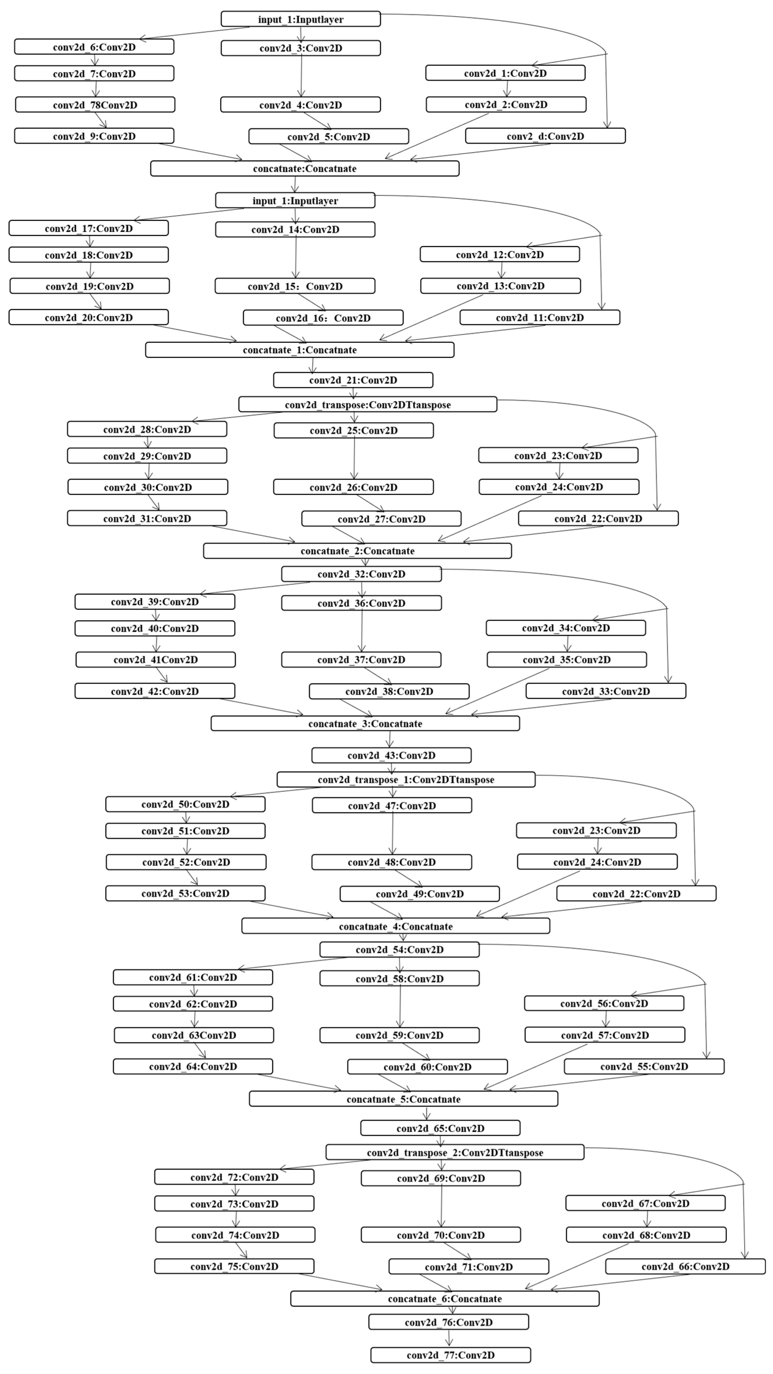
The super-resolution algorithm is based on a convolutional neural network trained by traditional gradient descent method to establish an end-to-end mapping model between a low-resolution image block and a high-resolution image block. The training process essentially involves learning the mapping between low-resolution images and real high-resolution images. When the error between the reconstructed image and the actual image reaches the expected value, the trained mapping can improve the resolution of additional images. On the basis of the classical PSRCNN model, we improved it to form the DSRCNN model. The new model has more network layers, resulting in better performance for the simulation. Figure 4 illustrates how the DSRCNN operation works.

By using bicubic interpolation, a single low-resolution image is zoomed three times to obtain a characteristic image, and then the output is obtained through network model processing. The goal of network training is to obtain accurate outputs, that are close to the original high-resolution image. The steps of network mapping include feature extraction, non-linear mapping, and reconstruction. Specifically, the low-resolution feature map is first obtained by convolving the low-resolution image, then the low-resolution feature map is mapped to the high-resolution feature block through non-linear mapping, and finally, the high-resolution feature block is reconstructed to obtain the high-resolution image.

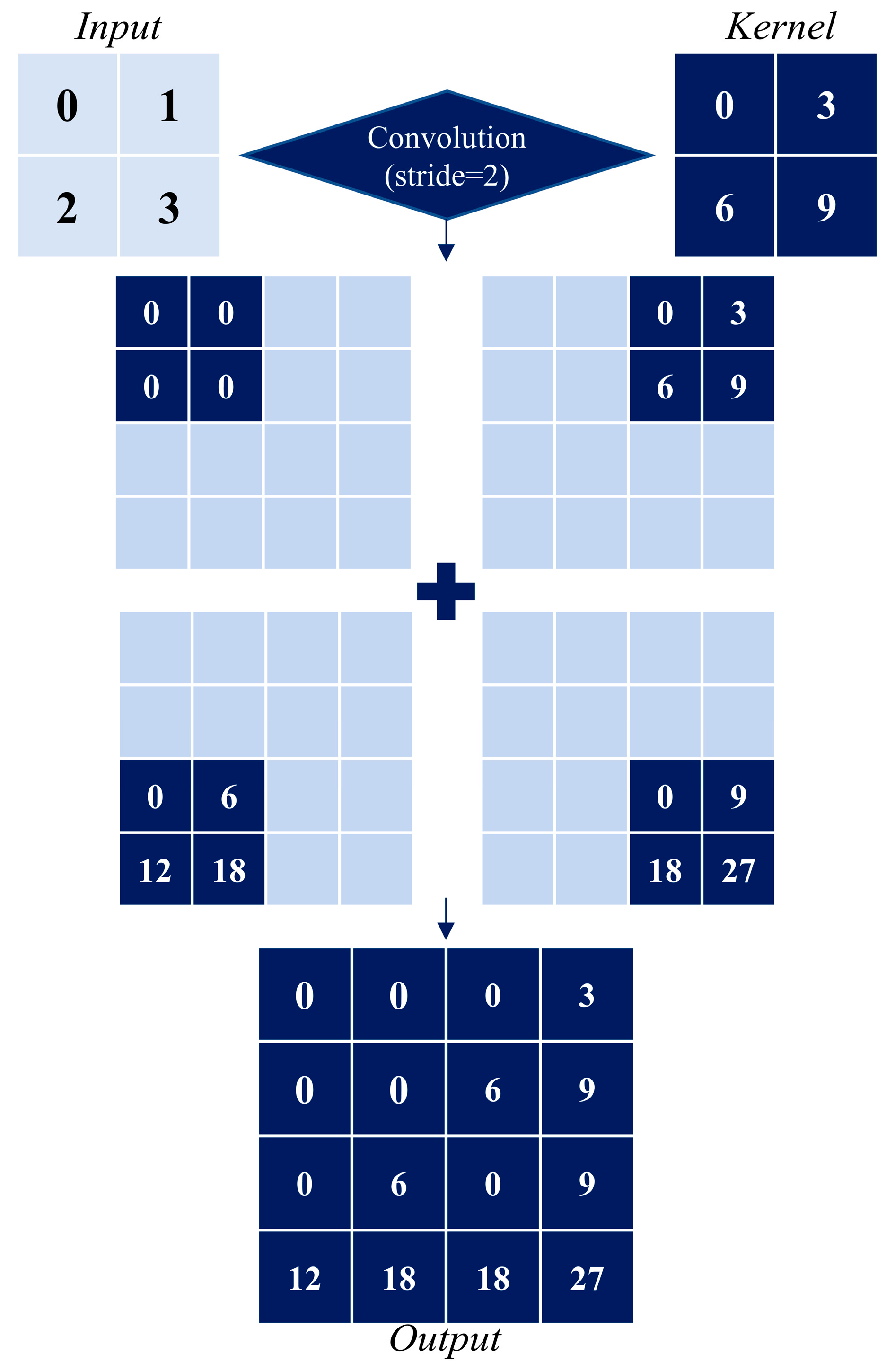
After feature extraction from low-resolution images using the convolution operation, the size of output results usually becomes smaller, which is not conducive to subsequent calculation and processing. The size of the input matrix can be restored by mapping the image from low to high resolution, which is called up-sampling. Conv2DTranspose is a method of up-sampling, an incomplete inverse process of convolution operation, and a component of non-linear mapping operation. Figure 5 illustrates the operation mode of the transpose convolution operation. The input quantity is a 2 × 2 matrix, the convolution kernel size is 3 × 3, the stride is set to 2, and there is no padding. The elements in the input quantity are multiplied by the kernel, and four intermediate tensors are generated by sliding the kernel in steps of 2 on the input quantity. Finally, by summing the four middle tensors, the output size of 4 × 4 is obtained. This significantly reduces the number of network layers, the computing costs, and the disk storage required. We utilized TensorFlow package and Keras to build a network, executed it in the Python 3.9 environment, and used NVIDIA GeForce RTX 3060 GPU (NVIDIA Corporation, Santa Clara, CA, USA) for the network training.

2.6.2. Transfer Learning

Traditional machine learning models have a strong dependence on the accuracy and representativeness of data, and are generally limited by the conditions of on-site data collection. This is because these technologies all rely on the common assumption that the source domain and the target domain have the same spatial characteristics and underlying distribution [46]. Inadequate data and unbalanced samples will greatly impair the accuracy of training results. Once the feature space and underlying distribution of the target domain change, it is necessary to recollect training data to train the model, which is costly in terms of computing cost resources [47].

Transfer learning is a machine learning method that uses the similarities between the old and the new domain to transfer the knowledge learned in the old domain to the new domain [48]. The old domain, the source domain, is a data set with a large number of training samples. The new domain, i.e., the target domain, is the object to be studied. The knowledge transfer from the source domain to the target domain completes the migration. New domains can be used when they are similar to the old ones; i.e., transfer learning allows source domains to be different from target domains [49]. Therefore, transfer learning can eliminate the limitations of the learning model and alleviate model over-fitting to improve the accuracy [50,51,52] and enhance the generalization ability of the model.

This study uses the Finetune method to transfer the model. When transferring the deep neural network, the front layer parameters of the neural network are fixed, the later layer parameters are pre-trained in the source domain, and the pre-training results are used as the basis to adjust the target domain. Because the parameters of the front layers of the new network model are determined by the source domain, the Finetune function will not change the front layers. The demand for data is greatly reduced, which solves the problem of insufficient training samples. We established a baseline model at the experimental scale and then applied it to real-world data using the transfer learning approach. Figure 6 represents the framework of transfer learning used in this study.

In this study, a 135° bend was established as the basic laboratory model. Then, the method of transfer learning was used to build a model of a 30° bend. Finally, the model of the real case (Xiaosi River) was established by using transfer learning.

2.7. Performance Metrices

The model fitting performance is represented using the root-mean-squared error (RMSE) and the coefficient of determination (R²), which can be expressed as

$$RMSE=\sqrt{\frac{1}{N}{\Sigma }_{i=1}^N{(f(x)-y)}^2}$$

(12)

$${\mathrm{R}}^2={\left|\frac{\mathrm{N}{\displaystyle \sum _{\mathrm{i}=1}^{\mathrm{N}}\left(f(x)\cdot y\right)}-{\displaystyle \sum _{\mathrm{i}=1}^{\mathrm{N}}\left(f(x)\right)}{\displaystyle \sum _{\mathrm{i}=1}^{\mathrm{N}}\left(y\right)}}{\sqrt{\left[{\displaystyle \sum _{\mathrm{i}=1}^{\mathrm{N}}\left(y^2\right)}-{\left({\displaystyle \sum _{\mathrm{i}=1}^{\mathrm{N}}y}\right)}^2\right]\left[{\displaystyle \sum _{\mathrm{i}=1}^{\mathrm{N}}\left(f{(x)}^2\right)}-{\left({\displaystyle \sum _{\mathrm{i}=1}^{\mathrm{N}}f(x)}\right)}^2\right]}}\right|}^2$$

(13)

where y are the ground truth data, f(x) are the predicted data, and N is the number of data pairs.

3. Results

3.1. Validation of the Hydraulic Models

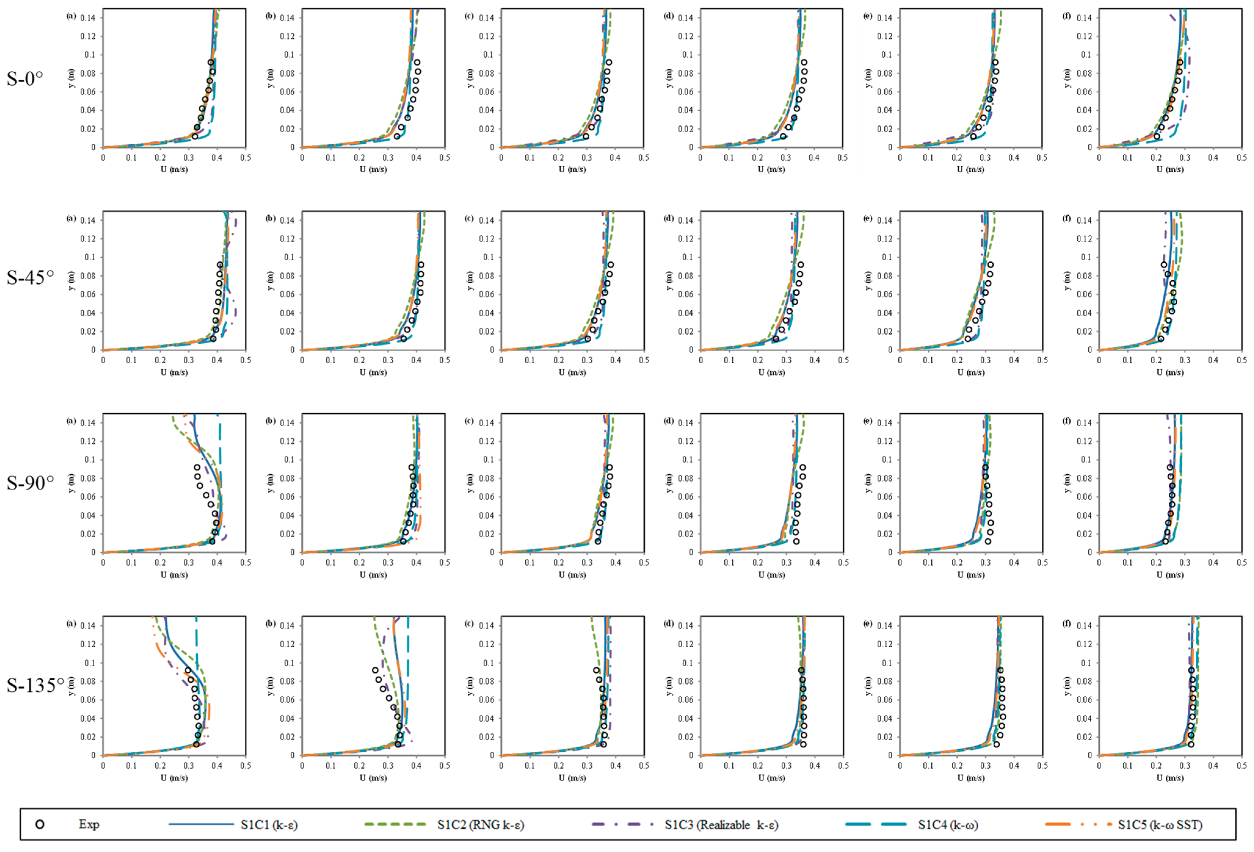
The vertical profiles of measured and simulated streamwise and transverse velocities at various locations are presented in Figure 7. The root mean square error (RMSE) values were also calculated. Specific values are as follows: S1C1 (k-ε) RMSE = 0.028 m/s; S1C2 (RNG k-ε) RMSE = 0.027 m/s; S1C3 (Realizable k-ε) RMSE = 0.023 m/s; S1C4 (k-ω) RMSE = 0.027 m/s. Generally, the agreement between measurements and simulations was quite good. The models performed relatively worse at locations S-90° (a) and S-135° (b), where the average RMSE values for the streamwise velocity exceeded 0.04 m s⁻¹. These two positions were located close to the inner bend. As expected and shown in the measurements, flow deceleration and the reversal of the vertical gradient of the velocity occurred at these locations. This phenomenon was predominantly induced by the unique helical flow pattern in channel bends: the cross-stream circulation in the bend affected the streamwise momentum, which in turn deflected the core of high velocities toward the outer bend [32,53,54,55,56]. The velocity profiles obtained by the Realizable k-ε model showed good matches with the data at these locations, but the other models were less accurate, implying that these models cannot satisfactorily capture the details of spiral flow structures observed in the laboratory test case. The plots also showed that the Realizable k-ε model performed consistently well at most locations near the outer bank, where an outer bank cell existed, implying that the Realizable k-ε performed better than the other models in the prediction of the outer bank flow distribution.

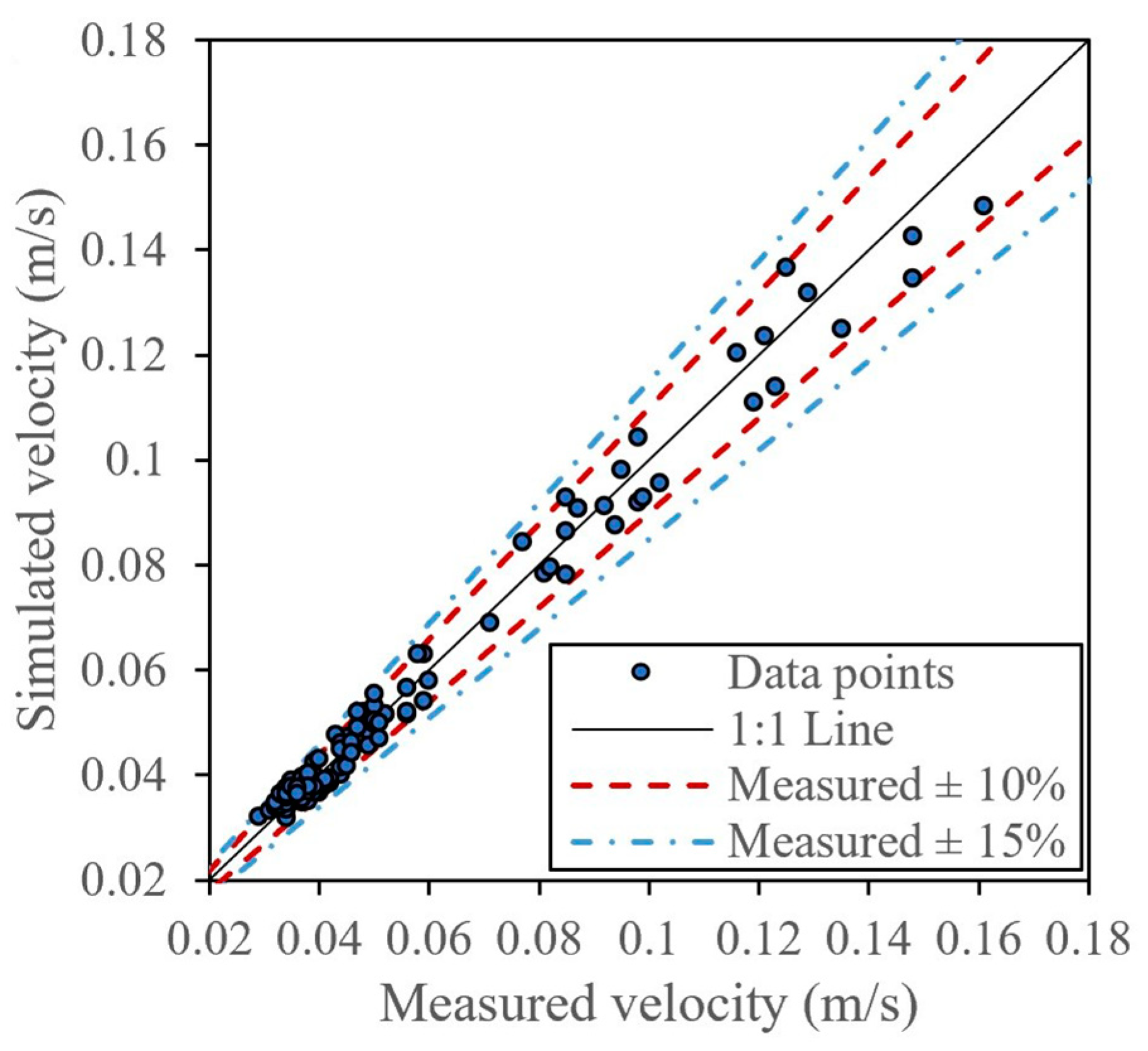
Figure 8 compares the predicted results and the Xiaosi River case. The accuracy of simulation results can be judged by the distance between points and lines, and the closer the data point is to the 1:1 line, the better the simulation effect is. It has been found that the deviation between the simulated value and the real value is mostly around 10% and within 15%. It can be clearly seen that the simulation data are similar to the real data, and their values are within a reasonable range, which indicates the satisfactory accuracy of the simulation. This indicates the value of the technology.

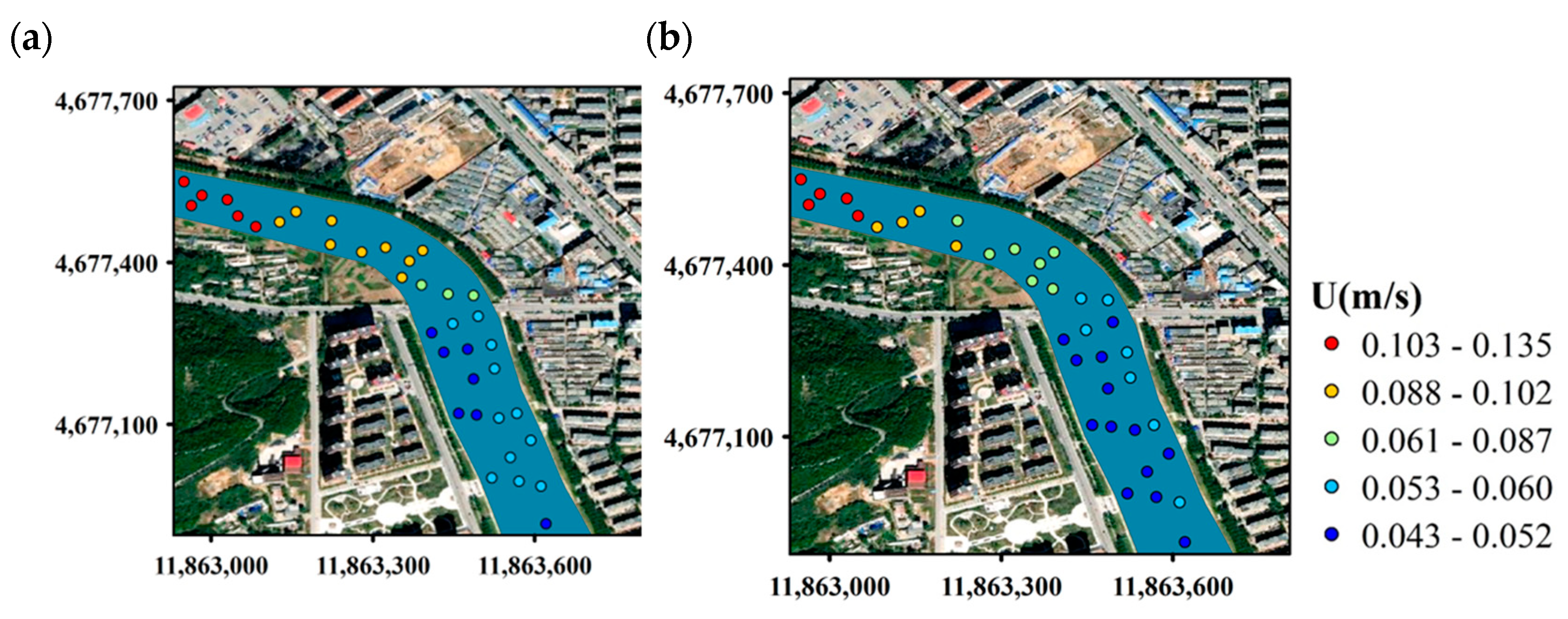
Figure 9 shows the predicted value and actual value of the same point. The color in the figure represents the flow value. In the comparison, we can see an obvious similarity here.

3.2. Prediction of the Flow Fields in Channel Bends Using the DSRCNN Model

As mentioned above, we established a hydrodynamic model and obtained low-resolution and high-resolution data. The low-resolution data and high-resolution data constitute a case under a specific upstream velocity. Different case data were established for different upstream flow velocity conditions at random to form a comprehensive data set, which can be used to train the DSRCNN model. The flow rate was divided into two flow components, U_x and U_z, to train the model. In the DSRCNN model, the input signal are low-resolution data and the output signal are high-resolution data.

The steps for our DSRCNN model training are as follows:

1.

Extract high-resolution data from the hydrodynamic model using ParaView and MATLAB;

2.

Use the Decimate function to extract low-resolution data from high-resolution data;

3.

Use low-resolution data from 20 cases as input matrices for 135° bends and 30° bends; low-resolution data from 10 cases are used for the Xiaosi River.

4.

Use high-resolution data from 20 cases as the target signal matrix for 135° bends and 30° bends; low-resolution data from 10 cases are used as the target signal matrix for the Xiaosi River.

5.

Train the DSRCNN by feeding the data of step (3) as input and enforcing the data of step (4) as the output signal.

After the DSRCNN model has been trained, further operations are required to verify the performance of the model since the simulation accuracy of the model has not been judged during the model training. To verify the performance of the DSRCNN model, it is necessary to generate high-resolution data and low-resolution data via the hydrodynamic model. Using low-resolution data as input, a simulation value was obtained after the DSRCNN model operation. The simulation value was compared with the high-resolution data generated by the hydrodynamic model to judge its performance. The specific operation steps are as follows:

1.

Extract high-resolution data from the hydrodynamic model using ParaView and MATLAB;

2.

Use the Decimate function to extract low-resolution data from high-resolution data;

3.

Use low-resolution data from 20 cases as input matrices for 135° bends and 30° bends; low-resolution date from 10 cases are used for the Xiaosi River.

4.

Using the data of step (3) as an input signal, predict the time-average velocity field of the validated bend by using the trained DSRCNN, and obtain the analog value matrix.

5.

Compare the analog value from step (4) with the target signal value from the low-resolution data.

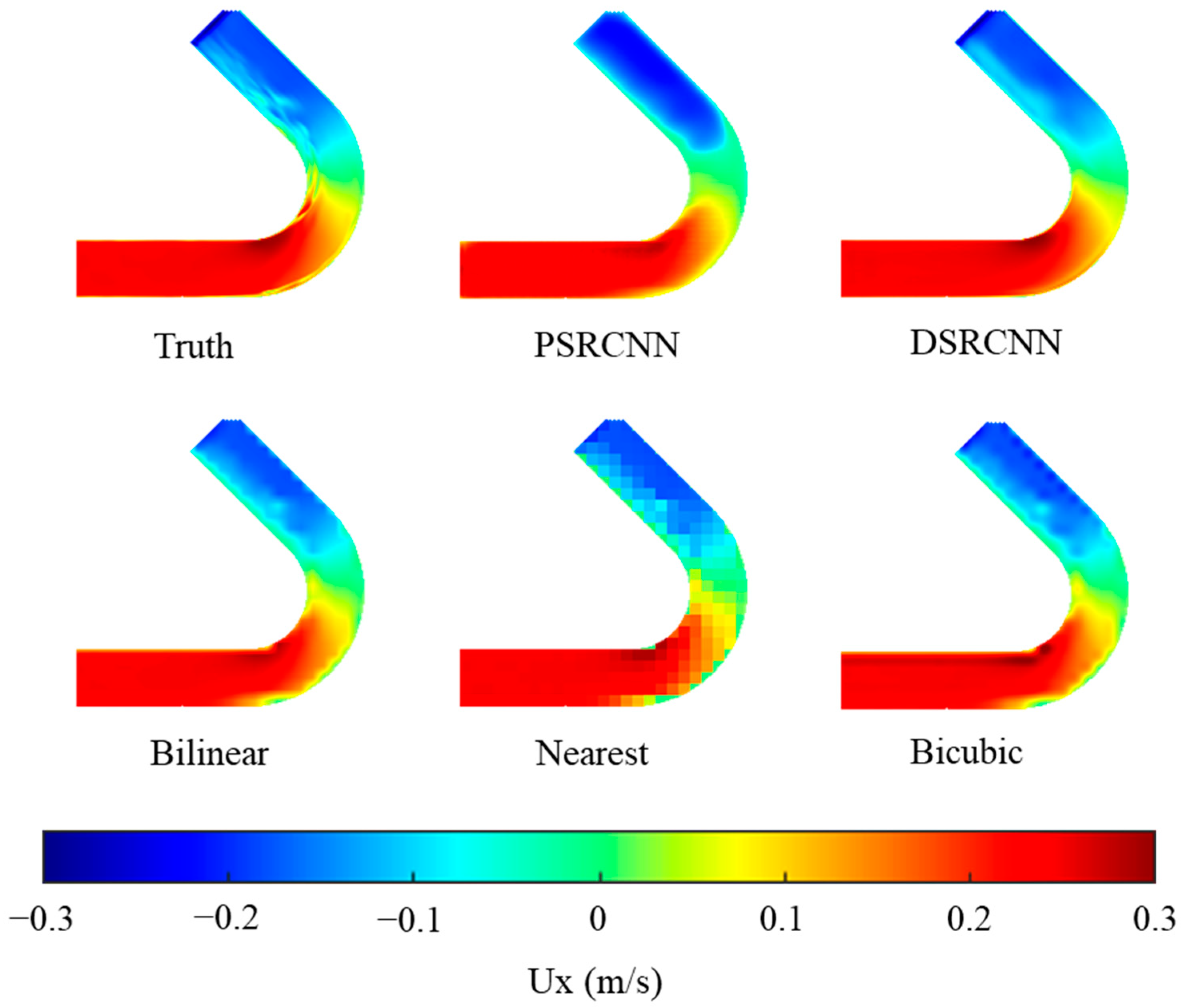
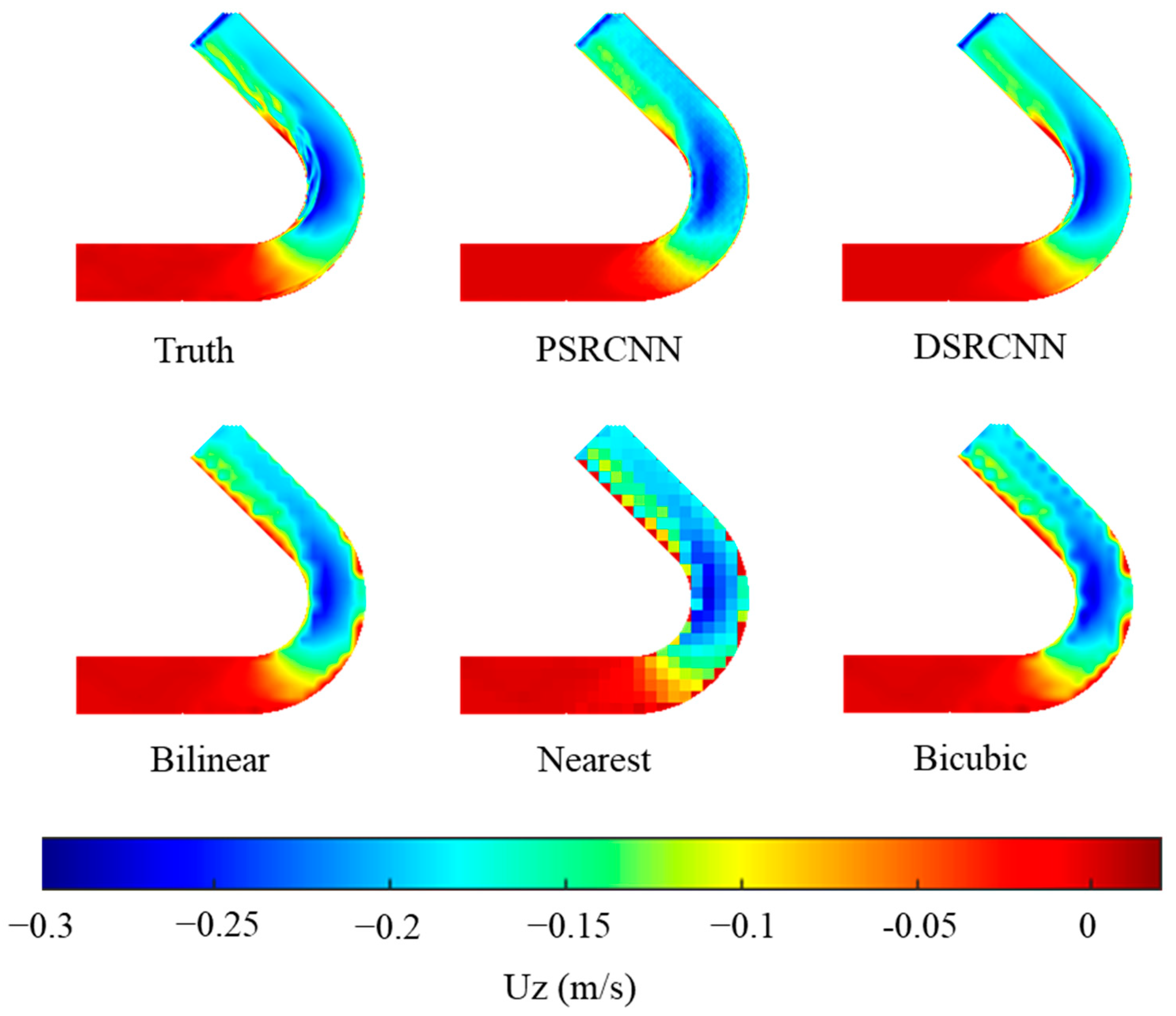
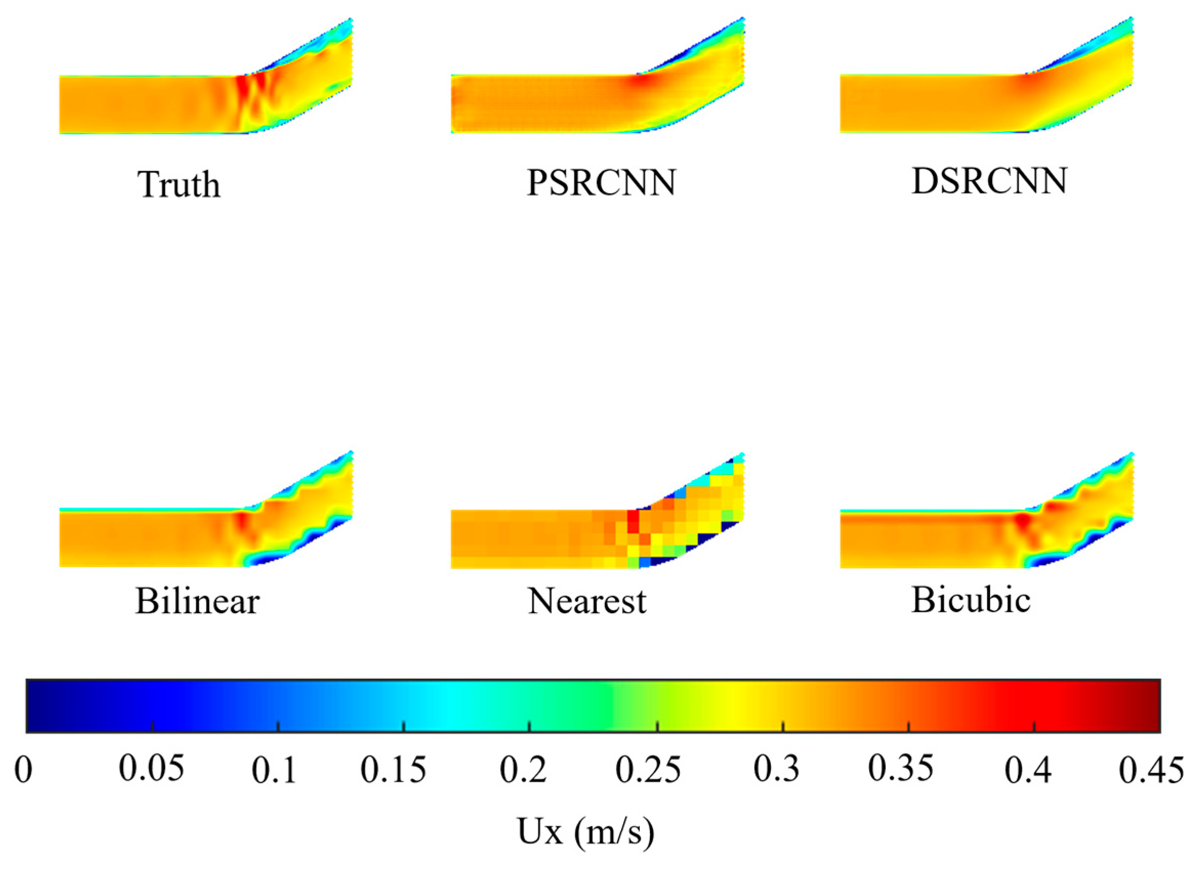
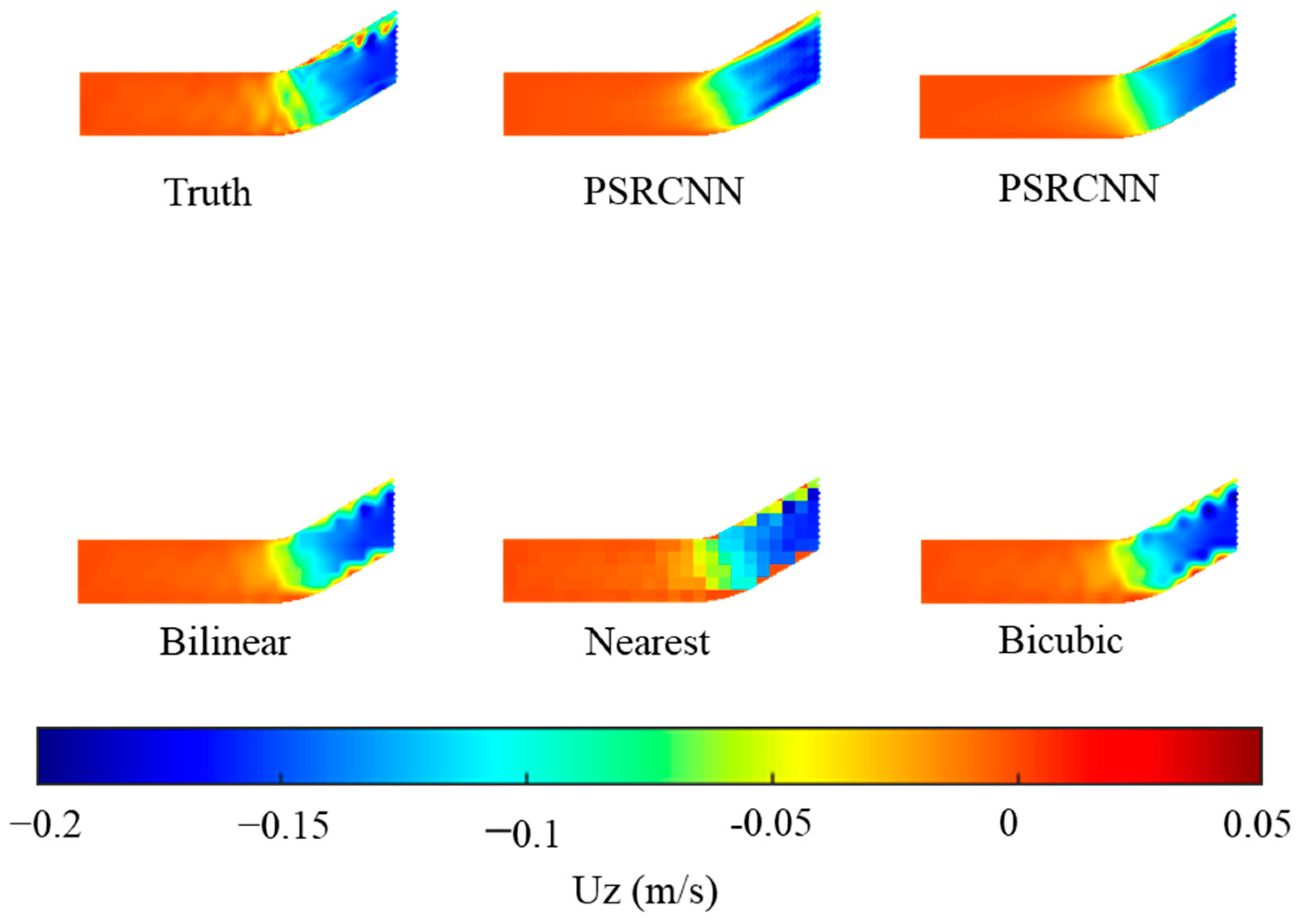
Figure 10 and Figure 11 show the flow field profiles of the predicted and actual high-resolution data, respectively, as obtained using the DSRCNN model with different velocity components in a 135° bend. We compared the PSRCNN model with the modified DSRCNN model to verify the improvement. At the same time, three commonly used spatial interpolation models were used, namely, Bilinear, Nearest, and Bicubic for data interpolation. The models and types used in this article are introduced in

Table 2. The models and types used in this article.

Model	Type
OpenFOAM	CFD
Delft3D	CFD
PSRCNN [57]	Deep learning
DSRCNN	Deep learning (the present study)
Bilinear [58]	Interpolation method
Nearest [59]	Interpolation method
Bicubic [60]	Interpolation method

. It can be seen that the predicted results of the DSRCNN model are very similar to the actual high-resolution results, and DSRCNN is the most satisfactory among the five methods in terms of improving the resolution.

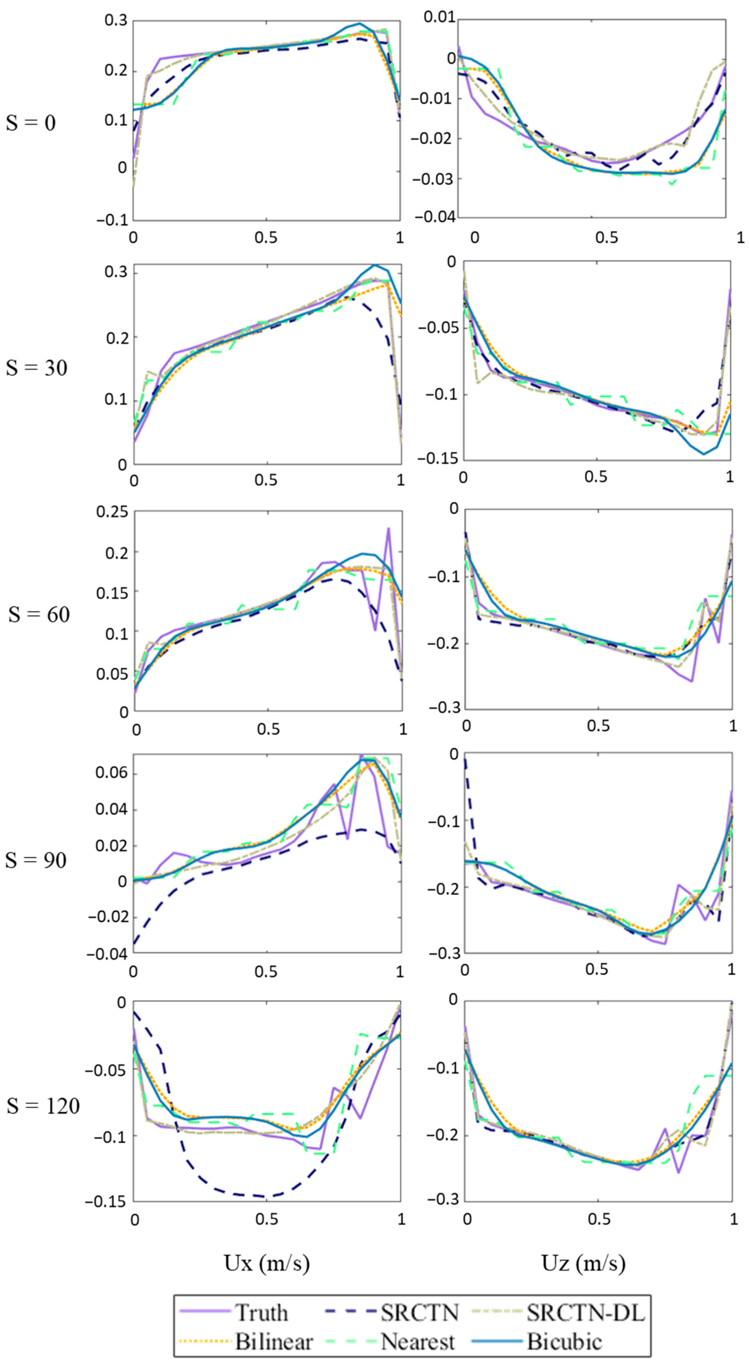
In Figure 12, the flow velocities at different sections of a bend are predicted using five different methods. Different colors represent different forecasting methods, and the component of flow velocity in two directions is shown separately. In the figure, a significant improvement in simulation accuracy can be found in the DSRCNN model.

Figure 13 and Figure 14 show the flow field profiles of the predicted and actual high-resolution data, respectively, as obtained using the DSRCNN model with different velocity components in a 30° bend. The results were also compared with the SRCTN model, Bilinear, Nearest, and Bicubic method. As can be seen in the figure, the prediction results of the DSRCNN model are satisfactory. In the front section at the bend, the water flow profile was not perfectly predicted by the DSRCNN model and SRCTN model, because the model smoothed the prediction and the DSRCNN model still exhibited the best overall performance according to the comparison of overall simulation results and error analysis.

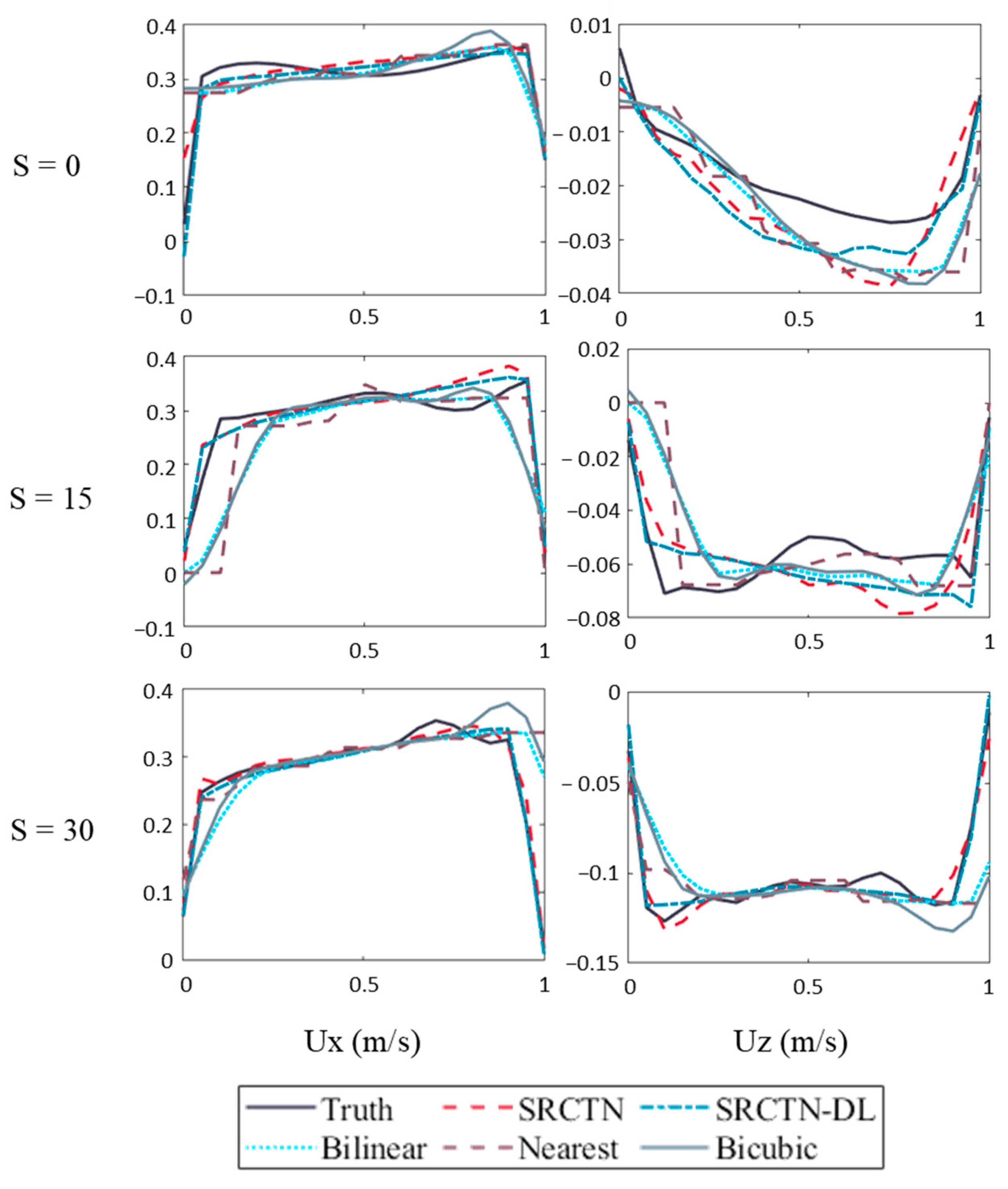
In Figure 15, the velocities were predicted using different methods in a 30° bend. In this figure, the DSRCNN model demonstrates superior performance in predicting various points.

3.3. Prediction of the Flow Fields in a Meandering River

The flow field simulation of the Xiaosi River uses the deep learning model of the 135° bend instead of starting from scratch. Even though there are some commonalities of water flow in both the 135° bend and the Xiaosi River, differences still exist; therefore, it is impractical for direct use. This can be solved using transfer learning. As we mentioned earlier, transfer learning can be used for similar types of data, such as images, video, biometrics, etc., and allows for differences, enabling transfer learning to be applied here. Before conducting transfer learning, it is necessary to establish a set of comprehensive data sets for the Xiaosi River. The comprehensive data set uses the previously verified Delft3D to establish the simulation of eight different cases. The upstream section flow corresponding to each case was 9, 12, 15, 18, 21, 24, 27, and 30 m³/s. Two cases were randomly selected as the transfer learning dataset, two cases as the validation data set, and four cases as the test data set.

1.

Use the validated delft3D model to generate data for different upstream section flows.

2.

Extract high-resolution data from the hydrodynamic model using ParaView and MATLAB;

3.

Use the Decimate function to extract low-resolution data from high-resolution data;

4.

Combine low-resolution data with high-resolution data to form a case. Eight cases are needed in this study;

5.

Randomly select two cases for transfer learning, and then use two cases for validation;

6.

The validated model uses the remaining four cases for testing.

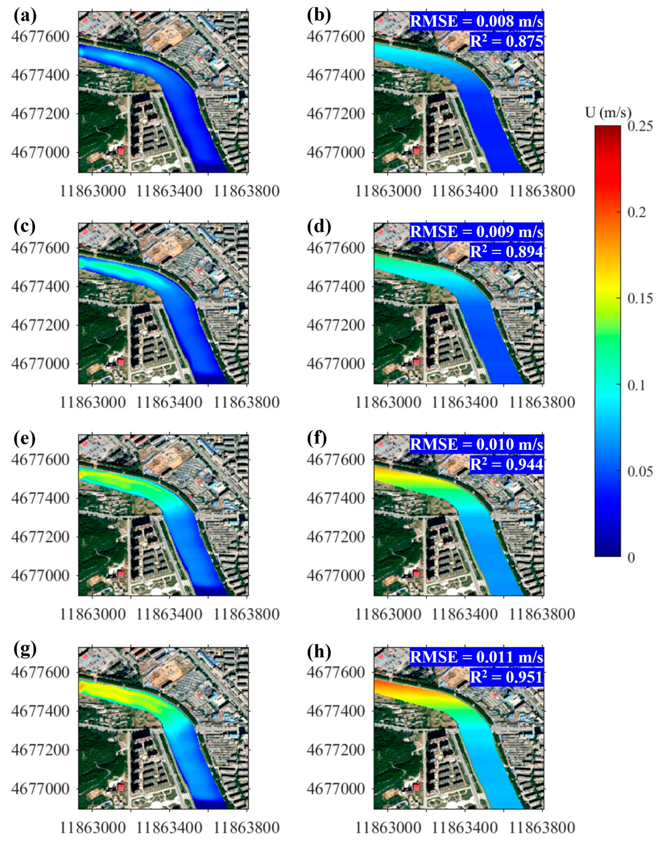
Figure 16 shows the spatial distribution of the flow pattern of the sample. The left one is the result of the numerical simulation, which is called ground truth, and the right one is obtained by using our deep learning algorithm. The trained model effectively reproduces the true distribution of water flow and has good simulation performance.

4. Discussion

The results have shown that DSRCNN has improved compared to PSRCNN, and DSRCNN has better simulation performance than three commonly used spatial interpolation models (Bilinear, Nearest, and Bicubic). The R² and RMSE between real data and simulated data indicate the good performance of simulating the flow field situation.

4.1. DSRCNN Transfer Learning

Three methods were used to conduct the 30° bend simulation:

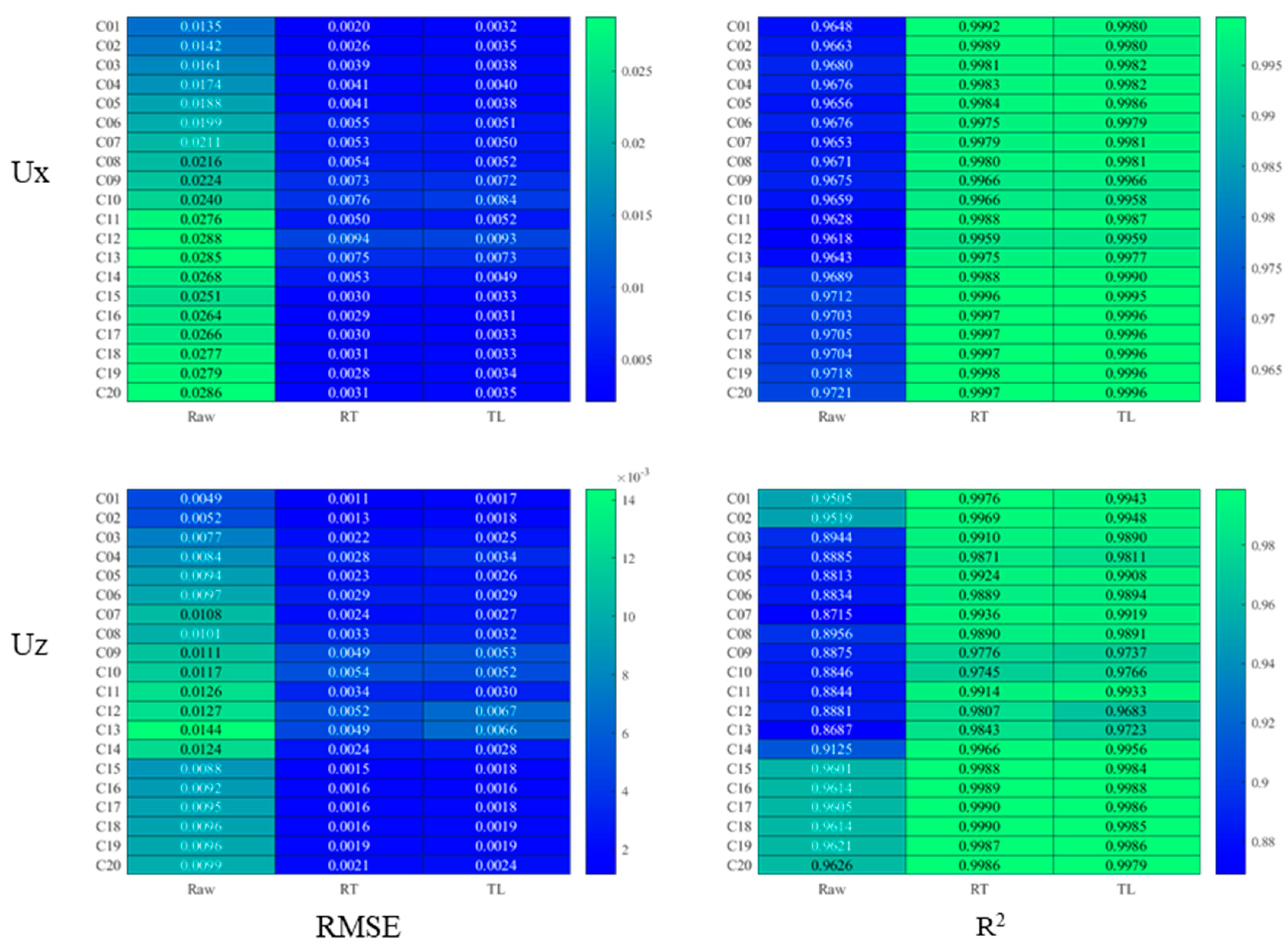
(1) The artificial intelligence model, trained using the comprehensive data set of the 135° bend experiment, was used for analysis, named Raw.

(2) The deep learning method was used to re-establish the comprehensive data set. At this time, the training result of the 135° bend was completely ignored, so it was named RT (return).

(3) The proven and powerful 135° model was combined with the transfer learning method, named TL.

It is worth noting that the amount of data used here was the same as that used in the 135° bend training case. The simulation results were obtained and analyzed with the actual values; both the RMSE and R² were calculated. We analyzed the flow of water in two directions, U_X and U_Z, and compared the performance of the three methods. In Figure 17, the results of 20 analyzed cases are displayed. It can be seen in the figure that the accuracy of the simulation results of RT and TR are generally satisfactory, while the simulation results of the Raw model are unsatisfactory.

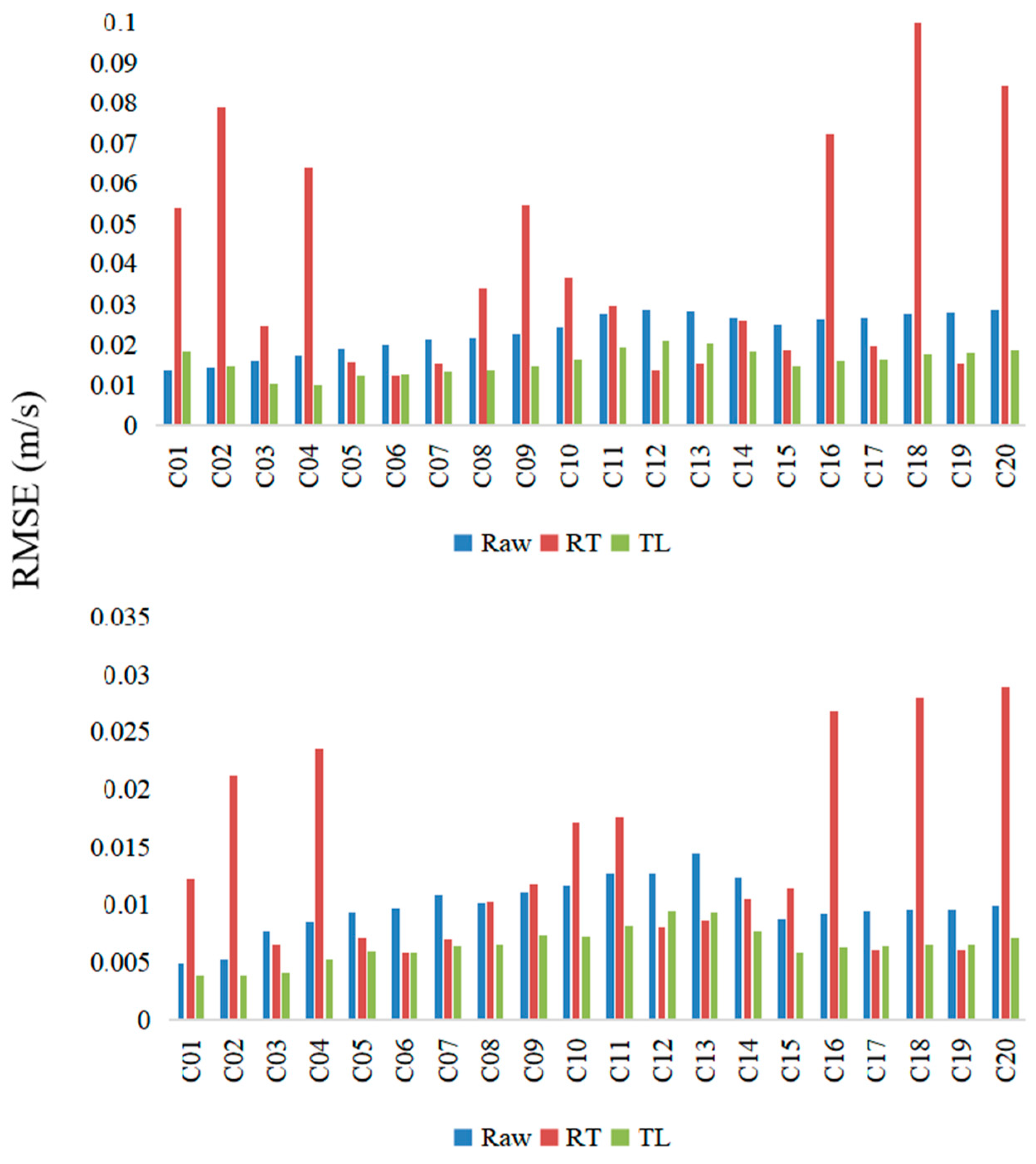
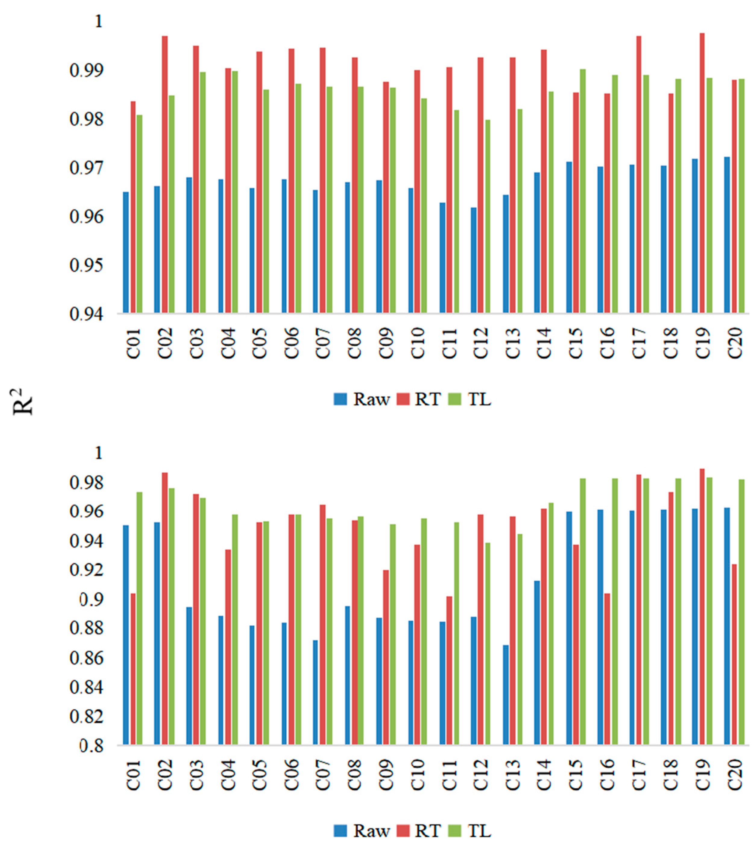
In order to further study the performance of the model when using a small amount of training data, we reduced the amount of training data. It was assumed that only two groups of data can be used for model experiments, that is, only two groups of data are used for model training, and two groups of data are used for validation, and the rest of the data are all used for testing. The RMSE and R² values of the three simulation methods are shown in Figure 18 and Figure 19. The error of transfer learning is generally the smallest, that is, its RMSE value is the smallest, and its R² is generally higher.

4.2. Merits and Limitations of the Approach

In the comparison between actual data and predicted data, we can easily find that both RT and TL produce acceptable results. But the result of the TL method has a smaller RMSE and its R² is closer to 1, indicating that the TL method is superior. For a small number of training cases, the TL method generally outperforms the RT method.

This research has developed an artificial intelligence model that can be processed with super-resolution and can obtain the flow field distribution of the research area based on a limited amount of observational data. The developed model can generate high-resolution flow field data based on low-resolution flow field data. The model achieved relatively accurate simulation results in both the laboratory and actual Xiaosi River studies.

One factor that restricts the application of the hydrodynamic model in the field of practical engineering is the computer time and storage requirements. Therefore, hydrodynamic models tend to incur significant computing costs in practical applications, which is unrealistic when the goal is to achieve real-time forecasting. By establishing the hydrodynamic model and validating it with the actual measured data, it was demonstrated that the data obtained by the hydrodynamic model can represent the actual flow characteristics of the river to a certain extent. In other words, the hydrodynamic model was considered as the flow characteristic data generator which can generate real data. The intelligent network was continuously trained with the data generated by the model, constantly exploring the deep relationship between the input value and the target value. After training, the input value could obtain the required output value through the interpretative equation obtained previously. In subsequent use, the data did not need to be generated by the hydrodynamic model; instead, the measured value was directly taken as the input term and the results were obtained directly by using the network. The experimental results effectively demonstrated the significance and effectiveness of this method.

The developed AI model has the significant advantage of using a small amount of local measurement data to simulate and obtain more accurate results, even when there are no local measurement data. This is because machine learning continuously learns the potential relationship between input and target values and provides complex mathematical expressions that can easily be re-programmed into other retyped programs, effectively applying the learned expressions. Transfer learning also provides the possibility for studies in areas without observational data. Once there are certain similarities in water flow, transfer learning can be used to solve problems in areas without data using the knowledge learned in areas with sufficient data to measure. The point to reiterate is that the data obtained do not necessarily fully match the measurements or the predictions obtained by training the hydrodynamic model, but it has been shown in the studies that these slight differences are completely acceptable and can be considered relatively accurate. The values of error indices calculated in the experiments have shown that it is feasible to use the super-resolution learning model based on a convolutional neural network as an alternative to the hydrodynamic model for new scenarios.

However, the machine learning model did not successfully capture the abnormal fluctuations at the entrance of the bend, and this error did not obviously occur in the interpolation method. This may be because the result of the model may be smoother, but it is better than others on the whole. In future research, we will use stricter physical constraints to more accurately simulate the abnormal flow in the key areas of sharp bends.

5. Conclusions

A new super-resolution architecture was developed and applied to the actual flow situation using transfer learning. The model was compared with traditional models (including PSRCNN, Bilinear, Nearest, and Bicubic), and a relatively good correlation with the actual situation was demonstrated. Then, transfer learning was carried out to evaluate the universality of the method, and a remarkable superior performance was found.

The remarkable advantage of this model is that it can be used for super-resolution processing, and the data of this research area can be obtained from a small number of observation points. Model debugging and simulation analysis were conducted for 135° and 30° bends and the Xiaosi River basin. For the 135° and 30° bend cases, OpenFOAM was used for the hydrodynamic model simulation, and for the Xiaosi River, the Delft3D model was used. The comprehensive dataset generated by the hydrodynamic model was used to train and validate the deep learning model. The results of the model comparison show that the model can simulate the flow field distribution of the bend flow better than the other methods.

To the best of the authors’ knowledge, DSRCNN was first proposed and applied in meandering rivers. In the simulation, it was also difficult to capture the flow fluctuation at the entrance of the bend. In future research, we will test different data processing methods and add more constraints to further improve the accuracy of the model simulation. And we will use transfer learning to simulate more complex cases.