Abstract
The nonlinearity nature of land subsidence and limited observations cause premature convergence in typical data assimilation methods, leading to both underestimation and miscalculation of uncertainty in model parameters and prediction. This study focuses on a promising approach, the combination of evolutionary-based data assimilation (EDA) and ensemble model output statistics (EMOS), to investigate its performance in land subsidence modeling using EDA with a smoothing approach for parameter uncertainty quantification and EMOS for predictive uncertainty quantification. The methodology was tested on a one-dimensional subsidence model in Kawajima (Japan). The results confirmed the EDA’s robust capability: Model diversity was maintained even after 1000 assimilation cycles on the same dataset, and the obtained parameter distributions were consistent with the soil types. The ensemble predictions were converted to Gaussian predictions with EMOS using past observations statistically. The Gaussian predictions outperformed the ensemble predictions in predictive performance because EMOS compensated for the over/under-dispersive prediction spread and the short-term bias, a potential weakness for the smoothing approach. This case study demonstrates that combining EDA and EMOS contributes to groundwater management for land subsidence control, considering both the model parameter uncertainty and the predictive uncertainty.
1. Introduction
Land subsidence is one of the most critical issues for groundwater usage. However, its modeling and prediction are challenging. This is because land subsidence is a highly nonlinear process with various uncertainties arising from observation errors; the limited available observations; the correlation between parameters; and aquitard properties such as the slow hydraulic head propagation, inelastic deformation, and the past-maximum effective stress (preconsolidation stress), which is updated over time. This study focuses on quantifying the uncertainties in model parameters and predictions, which is both scientifically and practically significant, thus providing insights into subsurface processes and decision making in groundwater management.
Uncertainty in land subsidence model parameters is quantified by finding many sets of model parameters that reproduce the observed subsidence within acceptable error ranges. This is an inverse problem and is addressed through data assimilation [1]. Typical data assimilation includes an ensemble Kalman filter (EnKF) [2,3], an EnKF with multiple data assimilations (EnKF-MDA) [4], an ensemble smoother (ES) [5,6], an ES with multiple data assimilations (ES-MDA) [7,8,9], and a particle filter [10,11,12].
In data assimilation, the balance between optimizing model performance and maintaining model diversity (diversity among ensemble members) is essential. Optimization improves the ensemble’s consistency with the target data but reduces the model diversity. Excessive reduction in model diversity may lead to overconfidence, as the ensemble appears to be more consistent with observations and suggests reduced uncertainty. An extreme case is an ensemble collapse, where iterative assimilation cycles homogenize the ensemble, all members become identical, and the ensemble becomes statistically insignificant [11]. Addressing the reduction in model diversity associated with optimization is essential to avoid underestimating or miscalculating the actual uncertainty in the system.
Kim and Vossepoel [12] focused on the ensemble size (the number of ensemble members) to maintain the model diversity for land subsidence data assimilation with a particle filter. If the ensemble size is small, the complex nature of land subsidence degenerates the insensitive parameters’ diversity because of the pseudo-correlation between the parameters and the simulation. It is important to ensure the diversity of the parameters that are insensitive to reproduction analysis, since they may be sensitive to prediction [13,14]. Jha et al. [6] found a case where the ensemble converged too quickly using ES for UGS gas reservoir surface displacement data in northern Italy. Their case implies that while data assimilation considers multiple model states simultaneously, premature convergence can occur if the model diversity is not sufficiently maintained, similar to the initial value dependence in deterministic inversion [15]. Refs [5,6,9] showed that the posterior ensemble is influenced by the quality of observation data, its utilization, and integration with forward analysis. Thus, to properly perform data assimilation for land subsidence, complex and specialized adjustments are necessary regarding parameter search range and hyperparameter settings [5]. Because of this, Kang et al. [16] described ES as unstable in highly complex problems. To overcome these limitations, attempts are underway to add an initial ensemble selection scheme to ES [16,17], but the algorithm is becoming more complex.
The greatest problem lies in the nonlinear and complex nature of land subsidence. Data assimilation methods that are adaptive to nonlinear problems and flexibly adjust the balance between optimization and model diversity maintenance are necessary to address the different scenarios and challenges in land subsidence analysis.
Evolutionary-based data assimilation (EDA) has never been applied to land subsidence but is a promising option. EDA is a data assimilation process using an evolutionary algorithm (EA), a population-based optimization method inspired by biological evolution [18]. The advantages of adopting EDA are as follows: First, EDA does not assume linearity or differentiability in the optimization problem, making it applicable to nonlinear land subsidence inversion. Second, since EA is a relatively classical optimization method, various approaches have been proposed to maintain the model diversity while advancing optimization, and EDA can take advantage of the accumulated knowledge. Recently, EDA has been studied for nonlinear problems such as the classical Lorenz model [19] and streamflow forecasting [18,20]. If EDA is available in addition to the existing data assimilation methods for land subsidence, a more appropriate approach can be selected depending on the situation.
This study investigates the capability of EDA to quantify the uncertainties in land subsidence model parameters through a case study in Kawajima (Japan), with a particular focus on maintaining the model diversity. In Kawajima, the authors previously developed a one-dimensional land subsidence model with a deterministic evolutionary algorithm [21]. Although the existing model elucidated the land subsidence mechanism caused by seasonal groundwater level fluctuations, quantifying the uncertainty in the model parameters and prediction was a remaining problem. EDA addresses the model parameter uncertainty.
Predictive uncertainty is quantified through an ensemble prediction consisting of members with equivalent confidence. An essential application of quantified predictive uncertainty is decision making [22]. Ideally, all potential predictions should be captured by identifying all the possible model parameter combinations. However, due to practical limitations, the number of predictive ensemble members may be too small, the prediction may be biased, or the predictive uncertainty may be underestimated or too overestimated to provide helpful information for decision making.
A promising solution is to transform ensemble predictions into predictive probability density functions (PDFs) while correcting for biases and variances in the original ensemble predictions through post-processing, as is often used in weather forecasting [23]. There are multiple advantages to using post-processed predictive PDFs instead of raw ensemble predictions: (1) Post-processed predictive PDFs can be interpreted probabilistically even if the number of original ensemble members is small; (2) it is expected to improve the predictive performance by correcting for the predictive bias and over/underestimated prediction spread; (3) the post-processed predictive PDFs become robust when the original ensembles consist of several ensembles with different governing equations, initial conditions, and boundary conditions. Developing different ensembles is possible because post-processing is independent of the ensemble-building process. For the same reason, post-processing can be combined with any data assimilation method. If post-processing can complement the potential drawbacks of the filter or smoother approach, post-processed predictive PDFs will outperform the raw ensemble predictions in predictive performance.
To the best of the authors’ knowledge, this study is the first to propose the post-processing of the ensemble predictions of land subsidence. The employed post-processing method is ensemble model output statistics (EMOS) [24], one of the standard statistical post-processing techniques in weather forecasting. EMOS outputs Gaussian PDFs using the linear regression of the mean and variance of the original ensemble predictions. Thus, the EMOS prediction loses the potential multimodality of the original ensemble predictions but inherits the time-series trends of the original ensemble predictions and benefits from the post-processing described above. The regression coefficients are determined by minimizing the average value of the continuous ranked probability score (CRPS) over a given period prior to the prediction. The CRPS is a statistical measure of the distance between the observed value and the predictive distribution. The EMOS prediction with the regression coefficients determined by minimizing the average CRPS corrects for predictive bias and over/under-dispersive spread of the original ensemble prediction.
EDA and EMOS can potentially contribute to land subsidence modeling, but their performance needs to be investigated due to the lack of relevant studies. There are two research objectives: (1) to validate the performance of EDA in quantifying uncertainty in land subsidence model parameters and (2) to validate the performance of EMOS in quantifying long-term predictive uncertainty. This study involves the application of EDA and EMOS in Kawajima (Japan). Model parameters and predictions generally have different purposes and uses for evaluating uncertainty. Therefore, there is no guarantee that the parameter ensembles estimated to characterize the subsurface will provide helpful predictions for decision making. Combining EDA and EMOS solves this problem because the model parameter uncertainty and the predictive uncertainty are quantified independently. This point is demonstrated through a case study in this paper.
The paper’s organization is as follows: Section 2 describes the methodology, including the development and adjustment of the combination of EDA and EMOS for the land subsidence modeling. Section 2 also briefly describes the authors’ previous work on field data and the existing deterministic model in Kawajima [21], which are transferred to the case study to examine the performance of the proposed method in this study. Section 3 presents the results and discussions of applying EDA to the land subsidence model in Kawajima. Section 4 describes the post-processing of the prediction of the ensemble constructed in Section 3. The results and discussions on EMOS operation are presented by comparing the raw ensemble predictions and EMOS predictions. In Section 5, multiple other factors are considered that can affect the modeling results. Section 6 describes the conclusions.
2. Methods
2.1. Vertically One-Dimensional Land Subsidence Simulator
In this study, we used the existing land subsidence simulator developed by [25]. The simulator performs a coupled analysis of saturated groundwater flow and vertical uniaxial soil deformation. The elastic deformation is described by linear elasticity, and the plastic (inelastic) deformation is described by a modified Cam-clay model [26]. This simulator was previously used in Tokyo [25] and Kawajima (Japan) [21]. Here, only the essential points are concisely introduced (see [21] for details).
The governing equation of the groundwater mass conservation law is as follows:
where is the water density (kg m−3) (assumed to be constant); is the initial void ratio (-); is the void ratio (-); is the hydraulic conductivity (m s−1); is the gravitational acceleration (m s−2); and is the pore pressure (Pa). The void ratio change is composed of the elastic component and the plastic component . The elastic change in the void ratio is linear with the effective stress changes. When the effective stress changes from to , is
where is the specific storage (m−1). Here, the compression is taken to be positive, and the effective stress is
where is the total stress. The plastic change in the void ratio is calculated using the modified Cam-clay model [26].
where is the compression index, and is the past maximum effective stress (preconsolidation stress). Note that during plastic deformation, the elastic component in the void ratio change is canceled out by (2) and the second term of (4), and only the first term of (4) remains.
2.2. Evolutionary-Based Data Assimilation (EDA)
EDA is a technique that formulates EA for data assimilation from a Bayesian perspective. Therefore, EDA procedures follow the EA procedures. Since the main focus of this study is an EDA exercise for land subsidence and not a formulation, see [18] for a detailed organization of EDA based on a Bayesian perspective.
EA is a population-based optimization method in which the components are described using biological evolution as an analogy. The given optimization problem is called the environment, the solution is called the individual, the set of solutions is called the population, and the evaluation of each solution is called the fitness. EA aims to acquire individuals with high fitness after many cycles of population evolution. Individuals in a population compete with each other based on fitness to improve their fitness in the next cycle.
We call the -th set of subsurface physical parameters as individual . The fitness of individual is defined as the inverse of the root mean square error (RMSE) between the observed and simulated subsidence:
where is the RMSE calculated by individual . The RMSE is the degree of agreement between the observed and simulated subsidence:
where is the total number of observed subsidence data, (m) is the observed subsidence at the -th timestep, and (m) is the simulated subsidence at the -th timestep by individual . Because the smaller RMSE means a better agreement between the observed and simulated subsidence, an individual with high reproducibility has a high fitness. Equation (6) defines the assimilation target data using a smoothing approach.
EA generates new individuals by mixing the parameters of existing individuals as a crossover analogy. The new individuals are called offspring, and the individuals to be mixed are called parents. The two parental individuals are selected probabilistically from the population through a virtual roulette [27] with the probability proportional to the fitness:
where is the probability that individual is selected as a parent, and is the population size. The probability of becoming a parent is based on competition; individuals better fitted to the environment are more likely to produce offspring.
The parameter values of the offspring are random weighted averages of the parents’ parameter values, and thus, the offspring inherits the characteristics of the parents. Furthermore, normal random numbers are added to the parameter values of the offspring. This analogy for mutation encourages model diversity maintenance and solution search to escape from the local solution. The process of offspring production is repeated until the cumulative number of offspring reaches the population size. The new population is more fitted to the environment and replaces the current population. This is the evolution of the population to fit the environment better and promotes the assimilation to the observed subsidence defined in (6). Thus, the evolution of the population is equivalent to model updating in the ensemble smoother based on the Kalman gain function considering all past observations. The cycle of generation and replacement of a new population is called a generation, which is equivalent to an assimilation cycle.
Specific individuals with higher fitness in a population are called elites. Passing the elites unchanged to the next generation prevents the loss of good individuals once found [28,29]. Elites are equivalent to an ensemble. Note that the elites are a subset of the population, while the nonelite individuals are the search points.
The evolution cycle homogenizes the elites and eventually causes ensemble collapse (Figure 1a without fitness sharing) because mutation is insufficient to maintain the model diversity. Thus, we added a fitness-sharing procedure [30], the most popular implementation that assists in maintaining model diversity. Fitness sharing modifies the fitness of all individuals downwardly according to the density of individuals in the solution space. In the optimization process with fitness sharing, individuals are aggregated toward better directions in the solution space while repelling each other. As a result, various local optimal individuals are found (Figure 1a).
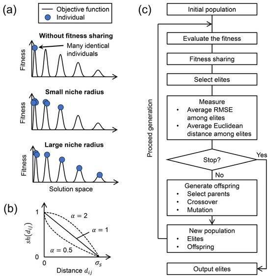
Figure 1.
(a) Conceptual scheme of fitness sharing; (b) sharing function; (c) flowchart of the implemented evolutionary multimodal algorithm.
The concept of fitness sharing is analogous, where each individual has a territory, and the individuals sharing the territory reduce each other’s fitness. The territory is called the niche, and the size of the niche is called the niche radius, which is the key to fitness sharing. The fitness reduction is significant when there are many individuals in a niche. The downward fitness modification of densely distributed individuals promotes model diversification and escape from local solutions by causing individuals to repel each other in the solution space.
Fitness sharing downwardly modifies the fitness of individual based on the total distance in the solution space between individual and all the individuals in the same niche. The fitness after the modification is calculated as
where is the population size, is the sharing function, and is the distance between individuals and in the solution space. The sharing function (Figure 1b) determines the degree of fitness modification based on . The sharing function is defined as
where is a constant, typically set to 1 [28,31], that determines the shape of the sharing function (Figure 1b), and is the niche radius. The sharing function strongly decreases fitness when an individual is similar to another. Note that the sum of denominators’ calculation in (8) includes the individual itself, so the denominator is never zero. Although the niche radius is a key factor controlling the strength of promoting model diversity (Figure 1a), setting an appropriate value is difficult [31,32,33,34,35,36].
Furthermore, is typically measured by the Euclidean distance [37,38]. If is the dimensionality of the solution space, the Euclidean distance normalized by the upper and lower bounds of each parameter is
where is the value of parameter of individual , is the value of of individual , is the upper bound of , and is the lower bound of .
Now, all the algorithmic components necessary for EDA are in place. Figure 1c shows a flowchart of the implemented EDA. A more specific algorithmic procedure is given in Appendix A. The algorithm aims to obtain diverse elites with comparable reproducibility of the observed subsidence.
- An initial population is prepared.
- All individuals are independently evaluated using (5) and (6).
- The fitness of all individuals is modified through fitness sharing (8)–(10).
- The number of individuals with the highest modified fitness are selected from the population as elites, where is the number of elites. Elites are copied to the empty population pool, where the population pool is the individuals that will be the population in the next generation.
- The average RMSE among elites and the average Euclidean distance among elites are measured to examine the assimilation status and model diversity. The average Euclidean distance among elites is calculated as follows:where is the normalized Euclidean distance between elites 𝑖 and 𝑗 calculated from (10). A decrease in 𝐷 implies a decrease in model diversity among elites.
- If the number of generations reaches the predetermined number of EDA termination generations, the procedure ends with the output of the elites at that point. Otherwise, the EDA procedure moves forward.
- Offspring is generated through parental selection, modified fitness, crossover, and mutation. The generated offspring is added to the population pool. The offspring generation and addition to the pool are iterated until the pool’s population reaches the population size.
- The population pool replaces the current population, and the procedure returns to the fitness evaluation (the second step).
The implemented EDA simultaneously promotes optimization and diversification for elites by performing generational iterations. The final output is diverse elites, i.e., diverse sets of model parameters with similar reproducibility of observed subsidence. The niche radius controls the intensity of diversification, with larger niche radii increasing diversification. The number of generations is equivalent to the number of assimilation iterations for the same dataset in ES-MDA.
2.3. Converting Ensemble Predictions to Predictive Probability Distribution Functions with EMOS
This section describes the ensemble model output statistics (EMOS) theory, which converts ensemble simulations into Gaussian PDFs. It also describes how to evaluate the conversion.
2.3.1. Theory of EMOS
The EMOS, proposed by [24], is a post-processing technique that transforms ensemble simulations into Gaussian PDFs while correcting for predictive bias and over/under-dispersive spread of the original ensemble. Since EMOS is a post-processing method, it can be applied to predictions by the parameter ensembles constructed by any type of inversion algorithm. It should also be emphasized that EMOS requires its own statistical training, independent of the construction of the parameter ensemble.
The main subject of EMOS is comparing the original ensemble prediction and the post-processed prediction. Here, we call the post-processed PDFs the EMOS distributions. The EMOS distributions cover both the ensemble assimilation period and the prediction period, where the ensemble assimilation period is the assimilation target period for the parameter ensemble, as defined in (6). Depending on the context, only the prediction period of the EMOS distribution may be of interest, in which case, the EMOS distribution is called an EMOS prediction.
If denotes the mean of the EMOS distribution for time , is a bias-corrected weighted average of the simulated values of the ensemble members at , as in (12).
where denote subsidence quantities at simulated by an ensemble consisting of members, is the time-independent bias parameter, and are time-independent non-negative weights of a linear regression. If denotes a variance of the EMOS distribution, is a linear function of the variance of ensemble simulation at , defined as
where is a time-independent coefficient, is a time-independent non-negative coefficient, and is the ensemble variance at . Combining (12) and (13) yields the EMOS Gaussian distribution as follows:
whose mean and variance depend on the ensemble simulation.
The most important part of the EMOS operation is the determination of the time-independent EMOS coefficients: and . The EMOS coefficients are determined by minimizing the average of the CRPS over a given period prior to the prediction. In this way, EMOS can correct for predictive bias and ensemble spread. The CRPS is a statistical measure of the distance between the point value and a distribution (not limited to a Gaussian distribution). The CRPS has the same unit as the point value and is defined as (15) [39]:
where is the point value, is a distribution, is the cumulative distribution function (CDF) of , and is the Heaviside function (16).
Figure 2 illustrates the concept of the CRPS using the observed cumulative subsidence and the EMOS Gaussian distribution as an example. The CRPS is small when the predictive PDF is sharp near the actual value. Conversely, if the predictive PDF is very dispersive, or if the predictive PDF is sharp but the peak is far from the actual value, the CRPS is large. If the prediction is very confident, i.e., in the case of the deterministic prediction, the CRPS is equivalent to the mean absolute error [39].
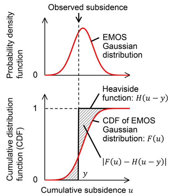
Figure 2.
The concept of CRPS using the observed cumulative subsidence and the EMOS Gaussian distribution as an example.
When calculating the CRPS for the EMOS distribution at time , is replaced by , which is the observation at time ; is replaced by the EMOS Gaussian distribution (14); and is replaced by the CDF of (14). In this case, the CRPS (15) can be expressed with a closed-form analytical solution [24] as follows:
where and denote the PDF and the CDF, respectively, of a Gaussian distribution with mean 0 and variance 1 evaluated at the normalized error . If is the observation for time from the time series of observation , the average CRPS over the period from to is calculated from (17) as follows:
where is the average CRPS over the period from to . Training EMOS or CRPS minimization refers to finding the time-independent EMOS coefficients and that minimize (18) for the specific period. This period from to is called the EMOS training period.
CRPS minimization allows the EMOS distribution to reasonably account for the variability in observations over the EMOS training period, i.e., correct for bias and the over/under-dispersive ensemble spread. When the ensemble spread is excessive relative to the training data, CRPS minimization tightens the EMOS distribution, but the variability in the training data does not allow for excessive tightening. Conversely, when the ensemble spread is underestimated relative to the training data, CRPS minimization widens the EMOS distribution, but the variability in the training data does not allow for excessive widening.
The EMOS coefficients were obtained by numerically minimizing (18) using the Broyden–Fletcher–Goldfarb–Shanno (BFGS) algorithm. A globally optimal solution is not guaranteed since the BFGS algorithm depends on the initial values. Thus, we prepared 40 sets of initial values and adopted the best result as the optimal solution. The 40 initial sets consisted of 39 randomly prepared sets and the simplest set from [40]: , equally weighted , , and . This is the simplest approach because the mean of the predictive Gaussian distribution is equal to the original ensemble mean, and the variance of the predictive Gaussian distribution is equal to the original ensemble variance. To constrain to be non-negative, the following procedure was used: First, (18) was minimized without any constraint on . If all were non-negative, the minimization was complete. If there were one or more negative coefficients, they were set to zero, and (18) was minimized again under this constraint. The ensemble variance was then recalculated using only the ensemble members remaining in the regression equation. Furthermore, the variance coefficients and must satisfy the non-negativity of (13) in addition to the non-negativity of . Although non-negativity was not required for , both and were obtained through optimization over and , which satisfied and .
2.3.2. Evaluation Criteria
The length of the EMOS training period affects the EMOS distribution [24]. Short training periods pose the problem of arbitrariness in the choice of training period. Long training periods cannot incorporate short-term biases. We shifted the EMOS training period to find the appropriate one and examined the predictive performance change. The evaluation criteria were (1) the empirical coverage, (2) the predictive coverage, (3) the RMSE, and (4) the CPRS. The RMSE was based on the EMOS mean (50% percentile). These criteria were used to measure the accuracy and sharpness of the predictive distributions. The definitions of the empirical coverage and predictive coverage are described below.
Coverage measures the proportion of actual values within certain probability intervals (PIs). If denotes a set of the central PIs from time to , is the % percentile, and is the % percentile of the ensemble simulation or the EMOS distribution at time . For example, when considering the 90% PIs for the ensemble simulation, the simulated member values corresponding to the 5% and 95% percentiles form the lower and upper bounds of the intervals. The PIs for the EMOS distribution are denoted in the same way. The indicator variable (19) is used to calculate the coverage of the PIs.
where is the observation for time from the time series of observation . Then, coverage over the period from to is defined as follows:
There are several types of coverage with different concepts, such as nominal, empirical, and predictive. Nominal coverage is for (19) and is predetermined using the modeler. Empirical coverage is the coverage over the EMOS training period, calculated as the percentage of training data falling within the % PIs to be trained. The significance of the empirical coverage is to test whether the % PIs explain % of the past observations. The predictive coverage refers to the predictive performance calculated by (20) over the prediction period. Ideally, the observations should be indistinguishable from random draws from the PDFs [23]. Thus, both the empirical and predictive coverage should match the nominal coverage. However, it is difficult to expect a complete agreement between the predictive and nominal coverage in long-term prediction. The reason is that nominal coverage expects a time-independent % prediction accuracy, whereas the predictive uncertainty typically increases over time (see [41] for a rigorous discussion).
2.4. Field Data Description: Kawajima, Japan
We applied this methodology to the field data in Kawajima town (Japan), where the authors previously reported the seasonally progressing land subsidence [21]. The previous work analyzed the land subsidence mechanism through a deterministic inversion for a one-dimensional model using an evolutionary algorithm without fitness sharing. Here, we briefly describe the work by [21] because this study performs an EDA using the same model domain, initial pore pressure distribution, boundary conditions, and observation data.
Kawajima is in the Arakawa lowland, where the entire surface layer is covered by Holocene deposits (as shown in Figure 3a,b). The surrounding surface layers consist of Pleistocene strata. The Arakawa River has eroded these Pleistocene strata and deposited sediments, forming the Holocene strata. Cross-sections of the north–south and east–west geological and hydrogeological profiles are shown in Figure 3c,d. The unconsolidated Holocene sediments have a 25–30 m thickness, posing a high risk of land subsidence due to groundwater extraction from shallow wells.
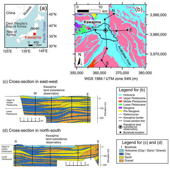
Figure 3.
(a) Location map; (b) surface geological map; (c) geological and hydrogeological cross-section in east–west; (d) geological and hydrogeological cross-section in north–south. Modified from [21].
Over 50% of the land use in Kawajima is agricultural, with most groundwater pumping occurring within a depth of 50 m. Agricultural groundwater usage during the summer significantly surpasses groundwater usage for other purposes. Consequently, groundwater levels exhibit seasonal fluctuations, primarily due to this seasonal pumping. This leads to a cyclical pattern of elastic expansion and elastoplastic compression of the ground each year, contributing to a cumulative process of land subsidence. Deformation data indicate that elastoplastic deformation is confined to formations between 0 and 80 m depth, while only elastic deformation is observed in deeper formations.
Groundwater levels have recovered in the long term, but land subsidence has progressed due to seasonal groundwater level fluctuation (Figure 4). Drought years have both sudden hydraulic head drop and significant subsidence due to increased water demand. The numerical model domain consisted of 87 meshes with nine types of layer classification (S, F1 to F5, and T1 to T3) (Figure 4c and Table 1). “S” represents the surface soil, “F” represents the aquifer, and “T” represents the aquitard. The following parameters were set for the layers so meshes belonging to the same layer would have identical properties: hydraulic conductivity (m/day), specific storage (1/m), the compression index (-), the initial void ratio (-), water density (assumed to be constant at 1000 kg/m3), solid density (assumed to be constant at 2600 kg/m3), and the overconsolidation depth (OCD) (m). The OCD is the past-maximum thickness of the overburden layer above the target layer [21]. The OCD is equivalent to the preconsolidation head at the initial condition. The preconsolidation head is the threshold hydraulic head below which inelastic compaction begins [42]. The simulation period was from January 1945 to April 2019, with a time step of one month. The hydraulic head shown in Figure 4a is a boundary condition set for the mesh at the observation screen’s center (Figure 4c). The surface mesh had atmospheric pressure. The bottom boundary had zero mass flux. The initial pore pressure distribution was hydrostatic, with a hydraulic head of 13.35 m. The initial preconsolidation stress distribution depended on the OCD. After estimating , , , , and OCD for nine layer types using evolutionary algorithm deterministic inversion, the model reproduced the observed subsidence with an RMSE accuracy of 3 mm.
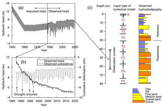
Figure 4.
(a) Hydraulic head for boundary conditions. The hydraulic head between 1945 and 1987 was assumed to account for the history of groundwater use and pumping regulation; (b) observed hydraulic head and observed land subsidence; (c) observation screen depths, nine types of layer classification of the numerical model, and observed hydrostratigraphy. Modified from [21].

Table 1.
Initially estimated parameter values of Kawajima model.
The model explained the land subsidence mechanism through three sets of layers:
- The first set was the aquifer consisting of F3, F4, and F5 with dynamically varying hydraulic head boundary conditions. Due to the thin clay layers in the aquifer, it had plastic deformations in drought years. The plastic deformation near permeable layers was essential to reproduce the significant subsidence that occurred only in drought years due to the sudden drop in the hydraulic head.
- The second set was T3, which had low hydraulic conductivity. T3 buffered the hydraulic head change propagating upward from the aquifer.
- The third set was F2 and T2, where the hydraulic head kept declining without seasonal fluctuations due to T3’s buffer. Due to the slow propagation of hydraulic heads, the aquifer’s long-term head recovery since the 1970s has not been transmitted to the third set, contributing to long-term subsidence.
Although the authors’ previous work [21] elucidated the land subsidence mechanism, the uncertainty quantification in the model parameters and the predictions remains challenging. The quantification of these uncertainties is essential in considering future groundwater management.
3. Quantification of Model Parameter Uncertainty Using EDA
In this study, we performed an EDA using a smoothing approach with multiple data assimilations for the same data, on a one-dimensional subsidence model in Kawajima to quantify the parameter uncertainty. The multiple data assimilations were used to evaluate the EDA’s ability to maintain the model diversity. The assimilation targets were the observed subsidence from April 1987 to April 2000 in Figure 4b. We used the same model domain, initial pore pressure distribution, boundary conditions, and observations as in [21]. The target parameters to quantify the uncertainty were the same as in [21], namely , , , , and OCD in the nine types of layers, and thus the dimensionality of the problem was 45.
3.1. Parameter Settings for EDA
Table 1 lists the initially predicted parameter set. We replicated it for the population size and used clones as the initial population. Table 2 shows the search range and standard deviation of normal random numbers for the mutation applied regardless of the layer type. Each parameter has upper and lower bounds to avoid unrealistic convergence. We set the standard deviation for mutation values that sufficiently explored the search range. Hydraulic conductivity and specific storage were explored on a logarithmic scale. If the mutated parameter value exceeded the limit, the parameter value was pulled back to the nearest limit.

Table 2.
Search range and standard deviation of normal random numbers for mutation.
Table 3 shows a hyperparameters setting for EDA. The population size was 1000. The number of elites was 500. The generational iteration (multiple data assimilations for the same data) was 1000 times. We prepared four values of niche radius with different orders of magnitude and performed the EDA independently with each niche radius. The intention was to compare multiple intensities that would prevent individuals from overcrowding. We determined the four values of niche radius through the following preliminary test: We repeated the EDA 100 times, advancing the generation only once in each run. Thus, we obtained 100 sets of populations that had advanced only one generation from the initial generation (we call each the first generation). Because the initial population consisted of clones of an initial prediction model in Table 1, the model diversity in the first generation only resulted from the mutation defined in Table 2. Thus, if the mutation intensities reasonably represented the search parameters’ uncertainty, the model diversity of the first generation would be a reference value for a niche radius that balanced the global and local search. Then, we measured the fluctuations in model diversity (the average Euclidean distance) from the 100 first-generation sets. The measured value range was 4.0 to 4.4. This way, four niche radius values of and were established with different orders of magnitude that could cover the 4.0-to-4.4 range. The niche radius setting of was particularly large because a single niche covered all first-generation models. The case without fitness sharing was also analyzed under the common settings in Table 1, Table 2 and Table 3 to compare the results with and without fitness sharing by simply skipping the fitness-sharing procedure.

Table 3.
Hyperparameter settings for EDA.
3.2. Ensembles Obtained Using Niche Radius: Results and Discussion
We performed the EDA independently for each niche radius setting. In each EDA run, 500 elites (the set of 500 elites was the parameter ensemble) were output. Here, we denote the ensembles assimilated with a niche radius of and as A1, A2, A3, and A4, respectively (Table 4). We denote the ensemble assimilated without fitness sharing as W. This section describes the EDA’s results and discussion: (1) the convergence status, (2) the obtained sets of model parameter distributions, (3) the agreement between observed and simulated subsidence, and (4) the ensemble predictions.

Table 4.
List of ensemble models obtained using EDA.
3.2.1. Convergence Status
To check the convergence status, we monitored the average RMSE among the elites and model diversity (average Euclidean distance among elites) over all generations. Figure 5a–e show the generational changes in RMSE and model diversity for A1 to A4 and W.
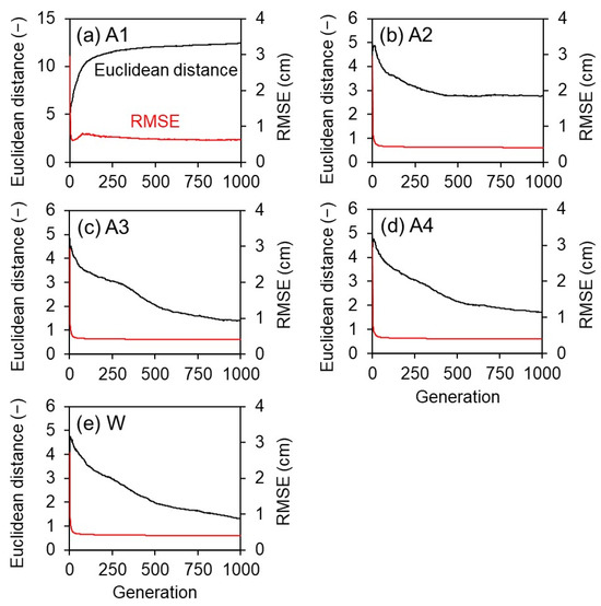
Figure 5.
Generational changes in the average RMSE among elites (red line) and the average Euclidean distance among elites (black line).
The RMSE behavior showed the convergence of assimilation for all parameters, A1 to A4 and W. The RMSE declined rapidly in the first dozen generations, suggesting that this period determined the overall direction of evolution. The Euclidean distance showed that EDA successfully maintained the model diversity for A1 and A2. The A1 model diversity increased with generation because a single niche covered all first-generation models. On the other hand, the model diversity in A3 and A4 continued to decrease, as did W without fitness sharing. Since the niche radius was not zero even in A3 and A4, the diversity could eventually reach equilibrium after more generations.
A2′s simultaneous convergence in the RMSE and model diversity implies that EDA reached an equilibrium between optimization and model exploration, making it impossible to explore new regions without new information. Notably, the equilibrium also implies that no matter how many times the assimilation was repeated for the same dataset, ensemble collapse did not occur, suggesting the EDA’s robustness. This equilibrium is due to the balance between the individuals’ aggregation to the local optima by creating genetically close offspring and the genetic counteraction from fitness sharing.
In summary, EDA took several dozen assimilation cycles to reach sufficient assimilation, and model diversity was maintained even after 1000 assimilation cycles for the same dataset. Note that, in ES and ES-MDA, it takes three or four assimilation cycles to reach sufficient assimilation (e.g., [9]), and the ensemble may suffer premature convergence (e.g., [6]). Although we did not directly compare EDA with other methods, Figure 5 implies that the implemented EDA may be dozens of times slower in assimilation efficiency than ES and ES-MDA but better at maintaining model diversity.
3.2.2. Obtained Parameter Sets
Figure 6 shows the model parameter distributions of A1 to A4 and W. The layer descriptions in Figure 6 correspond to the model domain’s nine layers in Table 1: S, T1, F1, T2, F2, T3, F3, F4, and F5 from the top layer. The gray lines represent the ensemble members’ parameter values, forming bands. Thus, the bandwidth represents the uncertainty in model parameters. Because A1 had the largest niche radius, its uncertainty was the highest. A2 was the next most uncertain, while A3, A4, and W were comparable in uncertainty. Overall, the estimated parameters were consistent with soil types: the aquifers tended to have higher hydraulic conductivity and stiffness than the aquitards, and no fatal convergence failures were identified.
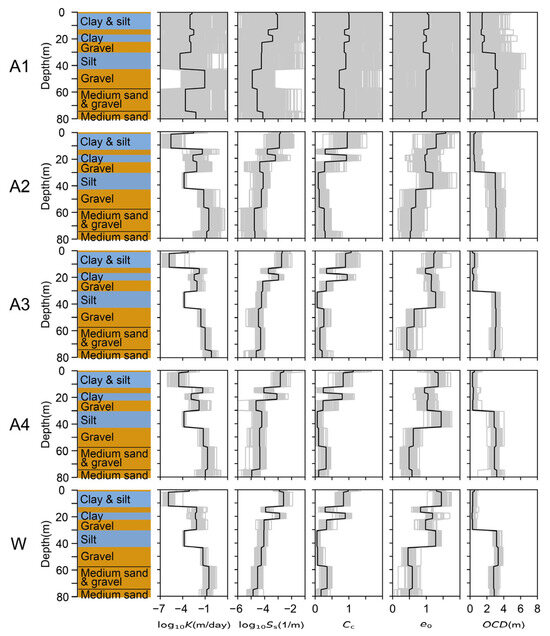
Figure 6.
Distribution of explored model parameters of nine subsurface layers. The black lines are the ensemble mean. The gray lines are the ensemble members.
Figure 7 shows the CDFs of hydraulic conductivity in F2, F4, and T3 and the compression index in T3. We chose these parameters because the reference core test results were available from the Geological Survey Report of the Kawajima Land Subsidence Observatory, compiled by the Water Quality Conservation Division (WQCD), the Department of Environment of Saitama Prefecture, in 1985 [43]. CDFs can show the distribution of the ensemble members within the parameter bands. For example, the parameter values on the horizontal axis corresponding to CDFs of 0.05, 0.5, and 0.95 were the 5%, 50%, and 95% percentiles of the parameter values, respectively. A1 had a wide range for all the selected parameters and did not provide a meaningful perspective on identifying physical properties.
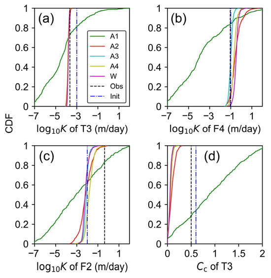
Figure 7.
Comparison of parameter CDFs between the ensembles, the observed value, and the initial value. (a) Hydraulic conductivity of T3. (b) Hydraulic conductivity of F4. (c) Hydraulic conductivity of F2. (d) Compression index of T3. The abbreviation “Obs” indicates observation, and “Init” is the initial value.
A2, A3, A4, and W showed the most successful constraint in the hydraulic conductivity of T3 (Figure 7a), which acted as a hydraulic buffer on the subsidence mechanism (described in Section 2.4). Although the initial estimation was ten times more permeable than the observed value, the ensembles were very well constrained close to the measurement value. Data assimilation without the assurance of maintaining model diversity may cause a fake uncertainty constraint. Thus, the uncertainty constraint under the EDA’s intense action of maintaining model diversity was remarkable.
The hydraulic conductivity of F4 also appeared well constrained (Figure 7b). However, since the initial estimation was nearly identical to the observed value, the constraint may be due to the initial value dependence. The initial value dependence was significant for the hydraulic conductivity of F2 (Figure 7c). This is because the pore pressure change in F2 driven by the boundary condition was buffered by the less permeable T3, making the hydraulic conductivity less sensitive to the reproduction analysis. The compression index of T3 converged lower than the measurement value, regardless of the initial estimation (Figure 7d).
3.2.3. Agreement between Observed and Simulated Subsidence
The agreement between the observed and simulated subsidence is plotted in Figure 8 to confirm the reproducibility and predictability of A1 to A4 and W. The ensemble simulations of A1 to A4 and W reproduced the long-term trend of the observed subsidence, which progressed cumulatively due to the seasonal groundwater level fluctuations. A1 had poorer reproducibility and a wide ensemble spread due to overemphasizing the model diversity rather than reproducibility.
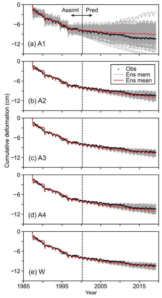
Figure 8.
Agreement between observed subsidence and ensemble simulations. The abbreviation “Assiml” indicates assimilation, “Pred” is prediction, “Obs” is observation, “Ens mem” is ensemble member, and “Ens mean” is ensemble mean.
3.3. Update of Ensemble with the Newly Available Observations
To validate the update of the ensembles with the new observations, we extended the assimilation period for A2 and performed EDA for 100 generations. Table 4 lists all the updated ensembles. The update procedure was carried out as follows: The extension of the assimilation period was five years. We used A2 as the initial population and obtained a new ensemble named B. We extended the assimilation period further and performed the same update process to construct ensemble C using B as the initial population. In the same way, we constructed ensembles D and E.
To check the assimilation to the new observations, we monitored the generational change in the average RMSE among elites and the average Euclidean distance among elites for an extended period. In the very early generations, there were sudden changes in the model diversity due to environmental changes, but it stabilized soon. There was no apparent change in the distribution of model parameters after updating. This is because there was not enough information in the new observations to tighten the model parameter uncertainty, as there were no notable long-term trend changes in the observed subsidence and observed hydraulic head (Figure 4b). In this sense, the fact that the update did not change the distribution of model parameters is a good indicator that the EDA prevented overconfidence in the ensemble.
Figure 9 shows the agreement between the observed and simulated subsidence for A2 and B to E. The new observations improved the ensemble reproducibility and the prediction spread, similar to ES [44].
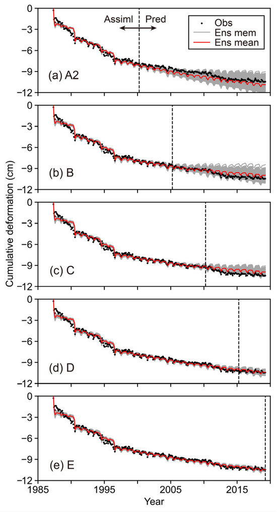
Figure 9.
Agreement between observed subsidence and updated ensemble simulation. The abbreviation “Assimil” indicates assimilation, “Pred” is prediction, “Obs” is observation, “Ens mem” is ensemble member, and “Ens mean” is ensemble mean.
3.4. Remaining Challenges and Possible Future Improvements for EDA
The challenge with the implemented EDA is the difficulty in determining the niche radius. A standard model diversity-preserving mechanism in other data assimilations includes artificial perturbations of observations based on measurement error. Since the niche radius is not directly related to the measurement error, it is not easy to estimate the niche radius that will achieve the desired ensemble reproducibility in advance.
Although EDA is adaptive to nonlinear problems, it is not easy to search the boundary area between feasible and unfeasible regions of the search space [45]. A simple solution is restricting the search space based on the core test results or the hydrogeological prior knowledge. A comparison with other data assimilation methods when applied to the same land subsidence problem is necessary to further investigate the EDA’s performance, as in [46].
In this study, we adopted an elastoplastic model to represent formation deformation. However, there are other possible constitutive models, e.g., an elastic–viscoplastic model [47,48]. The elastic–viscoplastic model is expressive in reproducing the creep process, which is a time-dependent, irrecoverable deformation under constant stress [47,49]. Since the creep process is highly nonlinear, it may be challenging to use ES and ES-MDA because they are unstable in highly complex problems [16]. Exploring the performance of EDA in different geological and hydrogeological settings will also enhance our understanding of its applicability. Further investigations are needed to address these points.
4. Quantification of Predictive Uncertainty Using EMOS
To test the EMOS’s performance in applying land subsidence ensemble prediction, we conducted EMOS training on the parameter ensembles obtained in Section 3. Then, we compared the predictive performance between the raw ensemble predictions and the EMOS predictions. Here, the EMOS distribution trained using ensemble “Name” is called “Name-EMOS”. For example, the EMOS Gaussian predictions acquired through post-processing “A2” is “A2-EMOS”.
The criteria used to evaluate the predictive performance were empirical coverage, predictive coverage, RMSE, and CRPS. The nominal coverage was 90%. Thus, the 90% PIs (90% probability intervals formed by the upper 95th percentile and lower 5th percentile of the raw ensemble predictions or the EMOS predictions) were the evaluation target for both the empirical coverage and predictive coverage. For the same reason, the ideal value for both the empirical coverage and predictive coverage was 90%. For comparison, we calculated the empirical coverage of the raw ensemble prediction for the same period as the EMOS training period.
The RMSE measures the agreement between the observed subsidence and deterministic predictions. We used the ensemble mean to calculate the RMSE for the raw ensemble predictions. We used the EMOS mean to calculate the RMSE for the EMOS predictions. For both the RMSE and CRPS, smaller values indicate better predictive performance.
Note that the predictive performance concerns the long-term prediction accuracy. The groundwater levels used for the boundary condition during the prediction period were the actual groundwater levels in the future. Therefore, for the predictive performance in this study, we assumed a perfect estimate of the future groundwater levels.
4.1. EMOS Results Using Different Ensemble Spreads
The EMOS training was performed for A1 to A4 by shifting the training period. The objectives were (1) to test EMOS’s performance on ensembles with different ensemble spreads and (2) to explore the appropriate EMOS training period. For shifting the EMOS training period, we analyzed 5 to 120 months prior to the prediction. Figure 10 shows the changes in the evaluation criteria when the EMOS training period was shifted.
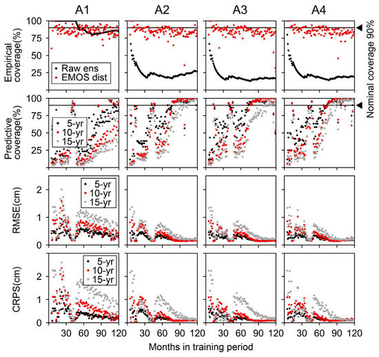
Figure 10.
Changes in empirical coverage, predictive coverage, RMSE, and CRPS as the EMOS training period was shifted. Legends are presented within each row. The abbreviation “Raw ens” indicates raw ensemble, “EMOS dist” is EMOS distribution, “5-yr” is 5-year prediction, “10-yr” is 10-year prediction, and “15-yr” is 15-year prediction.
4.1.1. Agreement between the Nominal Coverage and the Empirical Coverage
The empirical and nominal coverage (90%) agreement verifies the past statistical agreement between observations and distributions (ensemble simulations or EMOS distributions). Raw A1 had 100% empirical coverage for the 5–46-month training periods, meaning the ensemble spread was over-dispersive. Indeed, the parameter distribution (Figure 6 and Figure 7) and reproduction analysis (Figure 8) indicated that raw A1 was over-dispersive. On the other hand, raw A2, A3, and A4 had much lower empirical coverages than nominal coverage, indicating that the ensemble spread was under-dispersive.
After EMOS training, all A1-EMOS, A2-EMOS, A3-EMOS, and A4-EMOS exhibited approximately 80–94% of empirical coverage. This means that EMOS successfully corrected the ensemble spread, regardless of whether the original ensemble spread was over- or under-dispersive.
4.1.2. Change in Predictive Performance When Shifting the EMOS Training Period
The long-term predictive performance was assessed for the prediction horizon from 1 to 60 months ahead (5-year prediction), from 1 to 120 months ahead (10-year prediction), and from 1 to 180 months ahead (15-year prediction). Table 5 shows the predictive performance of raw A1, A2, A3, and A4. The predictive coverage of raw A1 was 100% for all of the 5-year, 10-year, and 15-year predictions because raw A1 was over-dispersive, i.e., the 90% PIs were too broad. This means that the prediction by raw A1 provides less meaningful information for decision making.

Table 5.
Predictive performance of raw A1–4. The unit for (predictive) coverage is %, and the unit for RMSE and CRPS is cm.
On the other hand, the predictive coverages of raw A2, A3, and A4 were below 58% for all of the 5-year, 10-year, and 15-year predictions. This is much lower than the 90% nominal coverage. The main reason for this low predictive performance was that the PIs with 90% coverage were too short, but the failure to capture the long-term trend due to bias also reduced the predictive performance. Better predictive coverage, RMSE, and CRPS were found in the 15-year prediction than in the 10-year prediction for raw A2, A3, and A4. This is because the systematic errors related to the Tohoku earthquake in March 2011, reported by [21], coincidentally acted as a bias correction to the long-term prediction trend since the earthquake.
A good EMOS prediction works robustly against the training period shift. The robust period maintains a similar output to other training periods. In this way, there is no confusion in the choice of the training period. The predictive coverage (Figure 10) had no robust training periods for the A1-EMOS. The reason was the significant reproduction error of A1 during the assimilation period, which made the EMOS training difficult. The A1-EMOS became sensitive to the training period shift, and the prediction bias was often corrected in the wrong direction, causing unstable predictive performance.
On the other hand, A2-EMOS, A3-EMOS, and A4-EMOS had good predictive performance in the 5-year and 10-year predictions, with training periods ranging from 74 to 101 months. Strictly speaking, the predictive coverage was stable at around 96%, which was slightly over-dispersive but satisfactory considering the long-term prediction’s difficulty and the raw ensembles’ poor predictive performance. When the training period exceeded 101 months, A2-EMOS, A3-EMOS, and A4-EMOS often had 100% predictive coverage in the 5-year and 10-year predictions. For the 15-year prediction, the training periods longer than 98 months showed good performance. Good predictive performance was also observed for the training periods of 39 to 47 months because the training data matched the trend of the verification data.
4.2. Comparison between Raw A2 and the A2-EMOS Trained over 92 Months
To examine the EMOS’s performance in detail, we compared the raw A2 ensemble and A2-EMOS trained over 92 months (September 1992 to April 2000) as a typical example from the robust training periods. Table 6 compares the evaluation criteria for the raw A2 ensemble and A2-EMOS. For all criteria, A2-EMOS was superior to raw A2. Figure 11 shows the 90% PIs of raw A2 and A2-EMOS. The EMOS mean captured the observations better than the ensemble mean of raw A2 until it was affected by the systematic error due to the Tohoku earthquake in March 2011.

Table 6.
Comparison of empirical coverage and the predictive performance for 5-, 10-, and 15-year predictions between raw A2 and A2-EMOS trained over 92 months (September 1992 to April 2000). The unit for empirical coverage and (predictive) coverage is %, and the unit for RMSE and CRPS is cm.
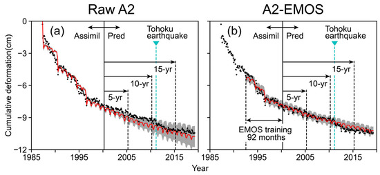
Figure 11.
Comparison of raw ensemble prediction and EMOS prediction: (a) 90% PIs of raw A2; (b) 90% PIs of A2-EMOS trained over 92 months. The red line in (a) is the ensemble mean. The red line in (b) is the EMOS mean. The gray area is the 90% PIs for both (a,b). Black dots are the observations for both (a,b). The abbreviation “Assimil” indicates assimilation, “Pred” is prediction, “5-yr” is 5-year prediction, “10-yr” is 10-year prediction, and “15-yr” is 15-yr prediction.
Notably, the predictive uncertainty of A2-EMOS remained constant over time. A2-EMOS with other robust training periods confirmed the same finding. This may be because raw A2’s ensemble spread was not constant for the time horizon. From 1995 to 2000, raw A2’s ensemble spread slightly increased. On the other hand, there was no such time trend in the observations. Thus, when training EMOS, the coefficient for the ensemble variance was not favorable, and the term constant over time was preferred, resulting in the constant EMOS prediction spread. Restrictions can be placed on and in CRPS minimization to prevent or obtain such a constant EMOS prediction spread (e.g., set to zero to prevent; set to zero to obtain).
4.3. EMOS for Updated Ensembles
To test the EMOS in practical situations, we conducted EMOS training on the updated ensembles B, C, and D using the past 92 months of observations. Figure 12a–f compare the reproduction and prediction between the raw ensembles and the EMOS distributions. The results indicate the necessity and difficulty of considering the seismic effects after March 2011. For example, the raw D predictions included biases that overestimated subsidence after 2015 (Figure 12e). D-EMOS trained over 92 months also failed to capture the observed trend after the earthquake (Figure 12f).
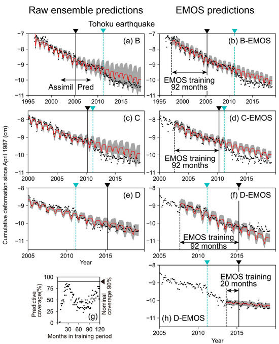
Figure 12.
Comparison of raw ensemble prediction and EMOS prediction: (a) 90% PIs of raw B; (b) 90% PIs of B-EMOS trained over 92 months; (c) 90% PIs of raw C; (d) 90% PIs of C-EMOS trained over 92 months; (e) 90% PIs of raw D; (f) 90% PIs of D-EMOS trained over 92 months; (g) the predictive coverage of D-EMOS when the EMOS training period was shifted; (h) 90% PIs of D-EMOS trained over 20 months. The gray area is the 90% PIs, the red line is the ensemble mean or EMOS mean, and the black dots are the observations for (a–f,h). The abbreviation “Assimil” indicates assimilation, and “Pred” is prediction.
Here, we show that EMOS with a short training period can correct the bias resulting from the seismic effect on the prediction. We conducted a training period shift for D-EMOS and checked the change in the predictive coverage (the prediction target was the observations from May 2015 to April 2019). Figure 12g shows the results. The EMOS prediction with a training period of 20 to 30 months showed good predictive performance due to intensive correction for the short-term bias. Figure 12h illustrates the prediction results of the D-EMOS trained over 20 months (September 2013 to April 2015). The bias related to the earthquake was successfully corrected. It should be noted, however, that the EMOS training became more sensitive to shifting the training period when it was shorter.
4.4. Strategies for Better and Robust EMOS Prediction
As mentioned in Section 4.1.2, it is preferred to train EMOS with the robust period, which maintains a similar output with other training periods. Sometimes, however, EMOS training against this basic strategy yields good results. As a short training period successfully removed the seismic effect from the prediction in Section 4.3, the modeler sometimes needs to subjectively set the training period depending on the situation (the observed data trend, the limitations of the numerical model, and the potential drawbacks of the filter approach or smoothing approach). In essence, the appropriate EMOS training period should be comprehensively determined by a modeler who understands the context of the problem.
Because EMOS is based on regression, it cannot correct for errors beyond the model representation. Thus, improving the predictive performance of the raw ensemble without relying too heavily on post-processing is essential for improving the EMOS predictive performance. Although not addressed in this study, predictions are robust when the ensemble is composed of ensemble members with different governing equations, initial conditions, and boundary conditions. In this way, ensemble predictions can incorporate various types of uncertainty. Because EMOS is independent of the ensemble construction process, it can output Gaussian predictions using mixed ensemble members. Indeed, this approach is standard in climate forecasts [50] and streamflow forecasts [51].
Raw ensemble predictions from EDA based on the smoothing approach can handle multimodal (multipeaked) predictions, but its short-term bias is one of its disadvantages. In addition, the spread of the EDA’s ensemble predictions is influenced by the niche radius, making its control challenging. On the other hand, EMOS prediction has superior bias correction, prediction spread correction, and interpretability. However, EMOS output is Gaussian distribution predictions, which greatly simplify the potentially valuable information that the raw ensemble predictions have. Thus, EMOS may oversimplify the representation of uncertainty in situations where predictions are not expected to gather around a mean value. Using EMOS for land subsidence prediction requires careful consideration of the specific modeling requirements and the nature of the uncertainties involved.
4.5. Scenario Analysis
We performed scenario analyses to demonstrate practices in groundwater management planning. The visualization of the predictive uncertainty helps decision makers consider whether the effort required to implement each scenario is worth the return obtained. Three hydraulic head scenarios prepared by [21] were used (Figure 13). Scenario 1 continued the seasonal fluctuation of the hydraulic head in 2019. Scenario 2 was half the seasonal variation in Scenario 1. Scenario 3 had the same seasonal fluctuations as Scenario 1, with a long-term trend of hydraulic head recovery (0.055 m/year). The hydraulic heads of all scenarios were smoothly connected to the observed head in April 2019 and were used as boundary conditions. Ensemble E, assimilated to all the data, was used to generate the predictions for each scenario.
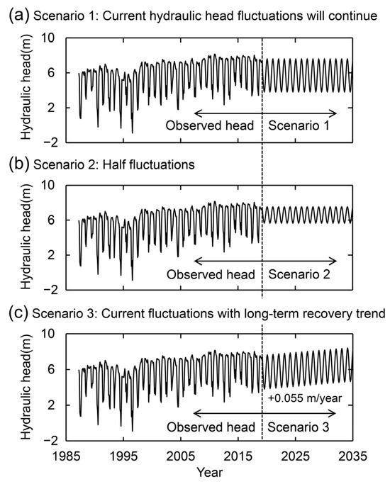
Figure 13.
Three scenarios of hydraulic head.
Figure 14 shows the scenario analysis results. The observed subsidence from mid-2014 to 2019 showed a relatively slow subsidence trend. On the other hand, the raw E simulation failed to capture the observed slow subsidence trend in the short term because of the smoothing assimilation of the long-lasting subsidence. The rapid subsidence bias of raw E needs to be corrected to make good predictions.
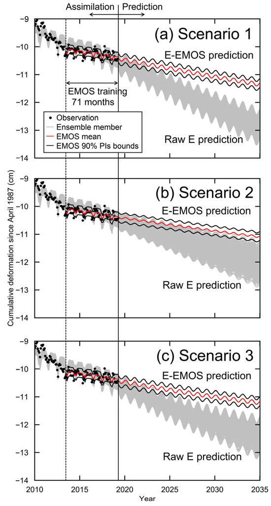
Figure 14.
Raw E prediction and 90% PIs of E-EMOS trained over 71 months for (a) Scenario 1, (b) Scenario 2, and (c) Scenario 3.
We conducted EMOS training on ensemble E over 71 months (June 2013 to April 2019). We chose this training period because (1) the training period after late 2013 corrected for the seismic effect on prediction in Section 4.3, and (2) the longer training period provided more stable training results.
The resulting E-EMOS 90% PIs (Figure 14) successfully captured the short-term trend of gradual subsidence from June 2013 to April 2019, and thus, good predictive performance was expected after 2019. Figure 15 compares the E-EMOS 90% PIs for Scenarios 1, 2, and 3. The mean subsidence rate was −0.59 mm/year for Scenario 1, −0.44 mm/year for Scenario 2, and −0.50 mm/year for Scenario 3. The width of the E-EMOS 90% PIs was nearly constant over time at 3.2 mm for all three scenarios because the EMOS coefficient for the ensemble variance was negligibly small. Similar results were obtained when the EMOS training period was shifted by several months.
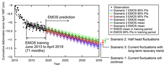
Figure 15.
The 90% PIs of E-EMOS trained over 71 months for Scenarios 1, 2, and 3.
5. Other Uncertainty Factors
This study primarily focused on model parameters and prediction uncertainties in land subsidence modeling. This section describes how we simplified multiple other factors that possibly influence modeling results.
Search parameter selection: We selected 45 parameters to explore, comprising five parameters (, , , , and OCD) in the nine types of layers. The selection considered the parameters’ relevance to the simulation results and the overall complexity of the inverse problem. Solid-phase density was assumed to be constant in all layers, but its influence was buried in the impact of other parameters. However, it might be considered in different geological and hydrogeological environments and at larger scales.
Geological, hydrogeological, and groundwater use homogeneity: We employed a vertical one-dimensional model. Stratigraphy is based on existing borehole data. This model domain structure assumes a horizontally homogeneous distribution of geology, hydrogeology, and groundwater use. In our case, the assumption is supported by the observation data in Section 2.4. Otherwise, a three-dimensional analysis is required.
Measurement error: Because the measurement errors of the borehole extensometer at Kawajima were not quantified in the existing studies, we could not add reasonable measurement errors and consider their possible effects on the inversion procedure. From another point of view, adding virtual measurement errors to the observation data in ES and ES-MDA is common. However, we did not apply it in EDA. Adding measurement errors aims to maintain the model diversity rather than accurately represent measurement errors. Indeed, the standard algorithm artificially expands the covariance matrix of the measurement errors using inflation factors, e.g., [8]. Furthermore, explicitly incorporating measurement errors into the algorithm does not guarantee that the reproduction errors of the resulting ensemble will match input measurement errors. In the sense that the goal is to maintain the model diversity, the EDA’s fitness sharing controlled by niche radius is an alternative to adding measurement errors. Although the niche radius is not directly related to measurement errors, its role in the algorithm is similar to inflation factors. Establishing an appropriate niche radius is difficult, as is determining the appropriate inflation factors.
It is crucial to recognize that data assimilation may make simulations consistent with observations even under invalid assumptions. The alignment might mask misinterpretations of underlying phenomena. A comprehensive examination of the consistency between observation data and modeling strategies will ensure that data assimilation does not merely fit models to observations but captures the essence of geophysical processes. The uncertainties and limitations mentioned above should be addressed in future studies.
6. Conclusions
The nonlinearity nature of land subsidence and limited observation data reduce model diversity during the data assimilation process, leading to both the underestimation and miscalculation of uncertainty in model parameters and prediction. EDA and EMOS are potentially promising solutions, but their performance has been unknown. This paper presented a case study in Kawajima with two research objectives: (1) to validate the performance of EDA in quantifying uncertainty in land subsidence model parameters and (2) to validate the performance of EMOS in quantifying long-term predictive uncertainty.
When performing EDA using a smoothing approach with multiple data assimilations, it took several dozen assimilation cycles for the ensemble to assimilate to the data sufficiently, and model diversity was maintained even after 1000 assimilation cycles for the same dataset. The balance of reproducibility and model diversity is controlled by niche radius, and in this study, the best balance was found in ensemble A2 with a niche radius of 1, which was well correlated to the mutation settings. The average RMSE of the reproduction analysis using A2 was 4.1 mm, indicating EDA’s high reproduction performance. The depth distribution of the estimated parameters was consistent with soil types. Assimilating new observations did not constrain the parameter uncertainty, but the predictive uncertainty was improved. Considering the overall results, EDA was excellent at maintaining the model diversity.
EMOS Gaussian predictions outperformed the raw ensemble predictions in predictive performance because EMOS compensated for the over/under-dispersive prediction spread and the short-term bias, a potential weakness for the smoothing approach, using past observations statistically. For example, in the 5-year prediction period following April 2000, the A2-EMOS 90% PIs trained over 92 months achieved better performance (coverage: 95%, RMSE: 0.16 cm, CRPS: 0.091 cm) than the raw A2 90% PIs (coverage: 31.7%, RMSE: 0.35 cm, CRPS: 0.21 cm). The raw ensemble predictions, influenced by the earthquake since 2011, tended to overestimate long-term subsidence. On the other hand, EMOS predictions with a short training period showed good predictive performance due to the effective correction of the short-term bias. Furthermore, scenario analysis using EMOS predictions showed that a groundwater management strategy that controls seasonal hydraulic head fluctuations reduces land subsidence more than a long-term hydraulic head recovery strategy.
There is no guarantee that the parameter ensembles estimated to characterize the subsurface will make helpful predictions for decision making. Combining EDA and EMOS solves this problem because the model parameter uncertainty and the prediction uncertainty are quantified independently, as was demonstrated in this study. The proposed methodology contributes to understanding and managing groundwater and land subsidence, considering both the model parameter uncertainty and the predictive uncertainty.
Author Contributions
Conceptualization, K.A. and M.A.; methodology, K.A. and M.A.; software, K.A. and M.A.; validation, K.A.; formal analysis, K.A.; writing—original draft preparation, K.A.; writing—review and editing, K.A. and M.A.; visualization, K.A.; supervision, M.A.; funding acquisition, M.A. All authors have read and agreed to the published version of the manuscript.
Funding
This research was funded by JSPS KAKENHI (Grant No. 21H01866), and the Cabinet Office, Government of Japan, Cross-ministerial Strategic Innovation Promotion Program (SIP), “Enhancement of National Resilience against Natural Disasters”.
Data Availability Statement
All the data needed to reproduce this paper and introductions on how to read the data are available in the following repository: Akitaya and Aichi (2023). Data observed at the Kawajima land subsidence observatory (Japan) and ensemble model (Version 2) [Dataset] are available in Zenodo at https://doi.org/10.5281/zenodo.8316450 (accessed on 5 September 2023). The developed Fortran code of the land subsidence simulator with EDA, a manual for using the compiled software, and a test problem to validate the software are available in the following repository: Akitaya and Aichi (2023). The code of the land subsidence simulator (LS3Dv3) with the inversion procedure of the evolutionary multimodal algorithm (Version 1) is available in Zenodo at https://doi.org/10.5281/zenodo.8316471 (accessed on 4 September 2023). The developed Fortran code of EMOS for land subsidence simulations, a manual for using the compiled software, and a test problem to validate the software are available in the following repository: Akitaya and Aichi (2023). The code of the ensemble model output statistics for land subsidence simulations (Version 1) is available in Zenodo at https://doi.org/10.5281/zenodo.8316500 (accessed on 4 September 2023). Figures in this paper were generated using Matplotlib Version 3.7.1 [52,53], available under the Matplotlib license at https://matplotlib.org/.
Conflicts of Interest
The authors declare no conflicts of interest.
Appendix A
Algorithm A1 shows a detailed overview of the implemented EDA. The EDA flowchart in Figure 1c shows that land subsidence simulations (“fitness calculation”) are performed on all individuals for simplicity. However, since the elites are individuals in which a subsidence simulation has previously been performed, there is no need to perform the subsidence simulation again if the calculation results are retained. To reduce the computational burden, Algorithm A1 is designed to perform subsidence simulations only on the offspring. Section 2.2 explains the specific implementation of each step of Algorithm A1. The developed Fortran code of the EDA with land subsidence simulator is available from the link in the Data Availability Statement.
| Algorithm A1 Evolutionary-based data assimilation with fitness sharing | |
| Input: Number of elites | |
| Output: Generational root mean square error among elites | |
| 1: | procedure EDA |
| 2: | Prepare one set of initial guess model |
| 3: | Evaluation on initial guess model |
| 4: | |
| 5: | |
| 6: | |
| 7: | for do |
| 8: | for , do |
| 9: | |
| 10: | through crossover between parent1 and parent2 |
| 11: | |
| 12: | |
| 13: | |
| 14: | end for |
| 15: | |
| 16: | Empty |
| 17: | |
| 18: | |
| 19: | |
| 20: | |
| 21: | end for |
| 22: | end procedure EDA |
References
- van Leeuwen, P.J. Nonlinear Data Assimilation for High-Dimensional Systems. In Nonlinear Data Assimilation; Van Leeuwen, P.J., Cheng, Y., Reich, S., Eds.; Springer International Publishing: Cham, Switzerland, 2015; pp. 1–73. ISBN 9783319183473. [Google Scholar]
- Wilschut, F.; Peters, E.; Visser, K.; Fokker, P.A.; van Hooff, P.M. Joint History Matching of Well Data and Surface Subsidence Observations Using the Ensemble Kalman Filter: A Field Study. In Proceedings of the SPE Reservoir Simulation Symposium; OnePetro: The Woodlands, TX, USA, 2011. [Google Scholar]
- Li, L.; Zhang, M. Inverse Modeling of Interbed Parameters and Transmissivity Using Land Subsidence and Drawdown Data. Stoch. Environ. Res. Risk Assess. 2018, 32, 921–930. [Google Scholar] [CrossRef]
- Emerick, A.A.; Reynolds, A.C. History Matching Time-Lapse Seismic Data Using the Ensemble Kalman Filter with Multiple Data Assimilations. Comput. Geosci. 2012, 16, 639–659. [Google Scholar] [CrossRef]
- Zoccarato, C.; Baù, D.; Ferronato, M.; Gambolati, G.; Alzraiee, A.; Teatini, P. Data Assimilation of Surface Displacements to Improve Geomechanical Parameters of Gas Storage Reservoirs. J. Geophys. Res. Solid Earth 2016, 121, 1441–1461. [Google Scholar] [CrossRef]
- Jha, B.; Bottazzi, F.; Wojcik, R.; Coccia, M.; Bechor, N.; McLaughlin, D.; Herring, T.; Hager, B.H.; Mantica, S.; Juanes, R. Reservoir Characterization in an Underground Gas Storage Field Using Joint Inversion of Flow and Geodetic Data. Int. J. Numer. Anal. Methods Geomech. 2015, 39, 1619–1638. [Google Scholar] [CrossRef]
- Le, D.H.; Emerick, A.A.; Reynolds, A.C. An Adaptive Ensemble Smoother with Multiple Data Assimilation for Assisted History Matching. SPE J. 2016, 21, 2195–2207. [Google Scholar] [CrossRef]
- Emerick, A.A.; Reynolds, A.C. Ensemble Smoother with Multiple Data Assimilation. Comput. Geosci. 2013, 55, 3–15. [Google Scholar] [CrossRef]
- Fokker, P.A.; Wassing, B.B.T.; van Leijen, F.J.; Hanssen, R.F.; Nieuwland, D.A. Application of an Ensemble Smoother with Multiple Data Assimilation to the Bergermeer Gas Field, Using PS-InSAR. Geomech. Energy Environ. 2016, 5, 16–28. [Google Scholar] [CrossRef]
- Gordon, N.J.; Salmond, D.J.; Smith, A.F.M. Novel Approach to Nonlinear/Non-Gaussian Bayesian State Estimation. In Proceedings of the IEE Proceedings F (Radar and Signal Processing); IET: London, UK, 1993; Volume 140, pp. 107–113. [Google Scholar]
- van Leeuwen, P.J. Particle Filtering in Geophysical Systems. Mon. Weather Rev. 2009, 137, 4089–4114. [Google Scholar] [CrossRef]
- Kim, S.S.R.; Vossepoel, F.C. On Spatially Correlated Observations in Importance Sampling Methods for Subsidence Estimation. Comput. Geosci. 2023. [Google Scholar] [CrossRef]
- Tonkin, M.; Doherty, J. Calibration-Constrained Monte Carlo Analysis of Highly Parameterized Models Using Subspace Techniques. Water Resour. Res. 2009, 45. [Google Scholar] [CrossRef]
- Herckenrath, D.; Langevin, C.D.; Doherty, J. Predictive Uncertainty Analysis of a Saltwater Intrusion Model Using Null-Space Monte Carlo. Water Resour. Res. 2011, 47. [Google Scholar] [CrossRef]
- Liu, Y.; Helm, D.C. Inverse Procedure for Calibrating Parameters That Control Land Subsidence Caused by Subsurface Fluid Withdrawal: 1. Methods. Water Resour. Res. 2008, 44. [Google Scholar] [CrossRef]
- Kang, B.; Jung, H.; Jeong, H.; Choe, J. Characterization of Three-Dimensional Channel Reservoirs Using Ensemble Kalman Filter Assisted by Principal Component Analysis. Pet. Sci. 2020, 17, 182–195. [Google Scholar] [CrossRef]
- Kang, B.; Lee, K.; Choe, J. Improvement of Ensemble Smoother with SVD-Assisted Sampling Scheme. J. Pet. Sci. Eng. 2016, 141, 114–124. [Google Scholar] [CrossRef]
- Dumedah, G. Formulation of the Evolutionary-Based Data Assimilation, and Its Implementation in Hydrological Forecasting. Water Resour. Manag. 2012, 26, 3853–3870. [Google Scholar] [CrossRef]
- Bai, Y.; Li, X. Evolutionary Algorithm-Based Error Parameterization Methods for Data Assimilation. Mon. Weather Rev. 2011, 139, 2668–2685. [Google Scholar] [CrossRef][Green Version]
- Dumedah, G.; Coulibaly, P. Evaluating Forecasting Performance for Data Assimilation Methods: The Ensemble Kalman Filter, the Particle Filter, and the Evolutionary-Based Assimilation. Adv. Water Resour. 2013, 60, 47–63. [Google Scholar] [CrossRef]
- Akitaya, K.; Aichi, M. Land Subsidence Caused by Seasonal Groundwater Level Fluctuations in Kawajima (Japan) and One-Dimensional Numerical Modeling with an Evolutionary Algorithm. Hydrogeol. J. 2023, 31, 147–165. [Google Scholar] [CrossRef]
- Doherty, J.; Simmons, C.T. Groundwater Modelling in Decision Support: Reflections on a Unified Conceptual Framework. Hydrogeol. J. 2013, 21, 1531–1537. [Google Scholar] [CrossRef]
- Gneiting, T.; Katzfuss, M. Probabilistic Forecasting. Annu. Rev. Stat. Appl. 2014, 1, 125–151. [Google Scholar] [CrossRef]
- Gneiting, T.; Raftery, A.E.; Westveld, A.H., III; Goldman, T. Calibrated Probabilistic Forecasting Using Ensemble Model Output Statistics and Minimum CRPS Estimation. Mon. Weather Rev. 2005, 133, 1098–1118. [Google Scholar] [CrossRef]
- Aichi, M. Land Subsidence Modelling for Decision Making on Groundwater Abstraction under Emergency Situation. Proc. Int. Assoc. Hydrol. Sci. 2020, 382, 403–408. [Google Scholar] [CrossRef]
- Roscoe, K.H.; Burland, J.B. On the Generalized Stress-Strain Behaviour of Wet Clay; Engineering Plasticity, Cambridge University Press: Cambridge, UK, 1968. [Google Scholar]
- Whitley, D. A Genetic Algorithm Tutorial. Stat. Comput. 1994, 4, 65–85. [Google Scholar] [CrossRef]
- Petrowski, A. A Clearing Procedure as a Niching Method for Genetic Algorithms. In Proceedings of the IEEE International Conference on Evolutionary Computation, Nagoya, Japan, 20–22 May 1996; pp. 798–803. [Google Scholar]
- Ursem, R.K. Diversity-Guided Evolutionary Algorithms. In Proceedings of the International Conference on Parallel Problem Solving from Nature, Granada, Spain, 7–11 September 2002; pp. 462–471. [Google Scholar]
- Goldberg, D.E.; Richardson, J. Genetic Algorithms with Sharing for Multimodal Function Optimization. In Proceedings of the Genetic Algorithms and Their Applications: Proceedings of the Second International Conference on Genetic Algorithms; Lawrence Erlbaum: Hillsdale, NJ, USA, 1987; Volume 4149. [Google Scholar]
- Das, S.; Maity, S.; Qu, B.-Y.; Suganthan, P.N. Real-Parameter Evolutionary Multimodal Optimization—A Survey of the State-of-the-Art. Swarm Evol. Comput. 2011, 1, 71–88. [Google Scholar] [CrossRef]
- Beasley, D.; Bull, D.R.; Martin, R.R. A Sequential Niche Technique for Multimodal Function Optimization. Evol. Comput. 1993, 1, 101–125. [Google Scholar] [CrossRef]
- Goldberg, D.E.; Wang, L. Adaptive Niching via Coevolutionary Sharing. Available online: https://citeseerx.ist.psu.edu/document?repid=rep1&type=pdf&doi=f872d929d49a2a5837a1361e543c41246532422d (accessed on 1 August 2023).
- Jelasity, M.; Dombi, J. GAS, a Concept on Modeling Species in Genetic Algorithms. Artif. Intell. 1998, 99, 1–19. [Google Scholar] [CrossRef]
- Shir, O.M.; Bäck, T. Niching with Derandomized Evolution Strategies in Artificial and Real-World Landscapes. Nat. Comput. 2009, 8, 171–196. [Google Scholar] [CrossRef]
- Fan, D.; Sheng, W.; Chen, S. A Diverse Niche Radii Niching Technique for Multimodal Function Optimization. In Proceedings of the 2013 Chinese Automation Congress, Changsha, China, 7–8 November 2013; pp. 70–74. [Google Scholar]
- Sareni, B.; Krahenbuhl, L. Fitness Sharing and Niching Methods Revisited. IEEE Trans. Evol. Comput. 1998, 2, 97–106. [Google Scholar] [CrossRef]
- Deb, K.; Goldberg, D.E. An Investigation of Niche and Species Formation in Genetic Function Optimization. In Proceedings of the Third International Conference on Genetic Algorithms; Morgan Kaufmann Publishers Inc.: San Francisco, CA, USA, 1989; pp. 42–50. [Google Scholar]
- Hersbach, H. Decomposition of the Continuous Ranked Probability Score for Ensemble Prediction Systems. Weather Forecast. 2000, 15, 559–570. [Google Scholar] [CrossRef]
- Grimit, E.P.; Mass, C.F. Initial Results of a Mesoscale Short-Range Ensemble Forecasting System over the Pacific Northwest. Weather. Forecast. 2002, 17, 192–205. [Google Scholar] [CrossRef]
- Christoffersen, P.F. Evaluating Interval Forecasts. Int. Econ. Rev. 1998, 39, 841–862. [Google Scholar] [CrossRef]
- Wang, G. New Preconsolidation Heads Following the Long-Term Hydraulic-Head Decline and Recovery in Houston, Texas. Ground Water 2023, 61, 674–691. [Google Scholar] [CrossRef] [PubMed]
- WQCD. Geological Survey Report of the Kawajima Land Subsidence Observatory; Water Quality Conservation Divsion, Depertment of Environment of Saitama Prefecture: Saitama, Japan, 1985. (In Japanese) [Google Scholar]
- Gazzola, L.; Ferronato, M.; Frigo, M.; Janna, C.; Teatini, P.; Zoccarato, C.; Antonelli, M.; Corradi, A.; Dacome, M.C.; Mantica, S. A Novel Methodological Approach for Land Subsidence Prediction through Data Assimilation Techniques. Comput. Geosci. 2021, 25, 1731–1750. [Google Scholar] [CrossRef]
- Michalewicz, Z.; Schoenauer, M. Evolutionary Algorithms for Constrained Parameter Optimization Problems. Evol. Comput. 1996, 4, 1–32. [Google Scholar] [CrossRef]
- Emerick, A.A.; Reynolds, A.C. Investigation of the Sampling Performance of Ensemble-Based Methods with a Simple Reservoir Model. Comput. Geosci. 2013, 17, 325–350. [Google Scholar] [CrossRef]
- Kelln, C.; Sharma, J.; Hughes, D.; Graham, J. An Improved Elastic–Viscoplastic Soil Model. Can. Geotech. J. 2008, 45, 1356–1376. [Google Scholar] [CrossRef]
- Ye, S.; Xue, Y.; Wu, J.; Li, Q. Modeling Visco-Elastic–Plastic Deformation of Soil with Modified Merchant Model. Environ. Earth Sci. 2012, 66, 1497–1504. [Google Scholar] [CrossRef]
- Kuhn Matthew, R.; Mitchell James, K. New Perspectives on Soil Creep. J. Geotech. Eng. 1993, 119, 507–524. [Google Scholar] [CrossRef]
- Tebaldi, C.; Knutti, R. The Use of the Multi-Model Ensemble in Probabilistic Climate Projections. Philos. Trans. A Math. Phys. Eng. Sci. 2007, 365, 2053–2075. [Google Scholar] [CrossRef] [PubMed]
- Duan, Q.; Ajami, N.K.; Gao, X.; Sorooshian, S. Multi-Model Ensemble Hydrologic Prediction Using Bayesian Model Averaging. Adv. Water Resour. 2007, 30, 1371–1386. [Google Scholar] [CrossRef]
- Hunter, J.D. Hunter Matplotlib: A 2D Graphics Environment. Comput. Sci. Eng. 2007, 9, 90–95. [Google Scholar] [CrossRef]
- Caswell, T.A.; Lee, A.; de Andrade, E.S.; Droettboom, M.; Hoffmann, T.; Klymak, J.; Hunter, J.; Firing, E.; Stansby, D.; Varoquaux, N.; et al. Matplotlib/Matplotlib: REL: V3.7.1 (v3.7.1); Zenodo: Geneva, Switzerland, 2023. [Google Scholar]
Disclaimer/Publisher’s Note: The statements, opinions and data contained in all publications are solely those of the individual author(s) and contributor(s) and not of MDPI and/or the editor(s). MDPI and/or the editor(s) disclaim responsibility for any injury to people or property resulting from any ideas, methods, instructions or products referred to in the content. |
© 2024 by the authors. Licensee MDPI, Basel, Switzerland. This article is an open access article distributed under the terms and conditions of the Creative Commons Attribution (CC BY) license (https://creativecommons.org/licenses/by/4.0/).