Waveform Imaging Based on Linear Forward Representations for Scalar Wave Seismic Data

Abstract

The current reverse-time migration, which is based on wave equations for imaging wavefields, employs an imaging formula derived from Claerbout’s imaging principle. This imaging formula is only valid for plane waves with small incident angles on the perfectly flat reflecting surface. However, the complexity of seismic wave propagation may lead to situations that do not meet this requirement. Therefore, this paper divides the subsurface into local scattering and reflecting bodies. It proposes linear forward representations for scattering and reflection data based on perturbations in the physical parameters and wave impedance, respectively. To further describe the effect on the reflecting body boundary, the local reflection coefficient is defined and the linear forward representation for the reflection data based on it is obtained. After that, the proposed linear forward representations are used as the forward equations for the linear inverse of the seismic data, and the seismic data waveform imaging method is developed based on linear inversion theory. At the same time, the specific waveform imaging calculation formulas for scalar wave scattering data and scalar wave reflection data are provided and validated via numerical experiments. Compared with the current reverse-time migration, waveform migration not only has the correct phase and higher resolution in theory but also does not increase the computational complexity. To some extent, it improves the deficiencies of the current structural imaging and provides a basis for subsurface lithological imaging.

1. Introduction

The concept of wave-equation migration imaging for primary seismic data originated in the early 1970s with Claerbout’s introduction of modern migration imaging [1,2,3]. It is one of the most important techniques in current seismic data processing and a primary method for obtaining 3D structural images of the subsurface [4,5,6]. The research and application of migration imaging have always been hot topics in seismic data processing. In recent years, classic reverse time migration has developed from scalar waves to acoustic and elastic waves, from 2-D models to 3-D models, using methods such as least squares or attenuation-compensation to enhance amplitude fidelity [7,8,9,10].

For optimizing the reverse time migration method, one research direction is to remove the low-frequency imaging noise. The most common method is filtering, including high-pass filtering, Laplace filtering denoising, directional attenuation denoising, Poynting vector denoising, and selective cross-correlation imaging denoising for wavefield direction [11,12,13,14,15,16,17]. Another research hotspot is to improve the computational efficiency, including the two-step explicit matching reverse time migration method, the Phase-shift time-stepping method based on Fourier transform, an efficient reverse time migration algorithm using a multi-step approach, and the one-step extrapolation method [18,19,20,21]. For developing the theory of migration imaging, some experts have proposed to consider imaging methods within the inversion theory, which develops conventional migration imaging into true amplitude imaging and least squares migration imaging [22,23,24,25,26,27,28,29]. Experts are also exploring reflection wave equation and scattering wave equation of reverse time migration in different media [30,31,32,33,34,35].

However, these methods retain the imaging conditions or formulas of reverse time migration, which is precisely what this paper aims to discuss. Seismic data objectively reflect changes in subsurface media, including travel-time and waveform information. In seismic exploration, seismic waves have a specific frequency band and corresponding wavelengths. Different wavelengths generate varied propagation types on the velocity boundaries in subsurface media. Therefore, when studying the changes in subsurface media using seismic data, the length of the seismic wavelengths must be considered. The forward representation for seismic data is the basis for constructing seismic wave inversion imaging methods, and different forward representations can lead to different inversion targets and methods. The theory of full waveform inversion (FWI) [36,37,38,39,40] highlights that lithology imaging in seismic data requires the effective use of both travel-time and waveform information. In essence, the inclusion of waveform information in seismic inversion results is crucial for advancing seismic inversion methods. To accurately use waveform information in migration imaging and to develop the current structural imaging towards lithology imaging targeting formation physical property parameters and reservoir parameters, we must construct a rigorous linear forward representation for seismic data based on wave theory.

Unlike conventional reverse time migration, which does not distinguish between scattering and reflection, the seismic data waveform imaging method proposed in this paper divides the subsurface into local scattering and reflecting bodies, and derived rigorous linear forward representations for scattering and reflection data based on perturbations in the physical parameters and local reflection coefficient, respectively. Another difference is that conventional reverse time migration is not based on inversion theory. The Claerbout’s imaging formula is a reflection coefficient calculation formula for plane waves with small angle incidents on an infinitely flat reflection interface. On the other hand, the waveform migration is developed on the basis of linear inversion theory and rigorous linear forward representations. In this way, it not only has the correct phase, more complete waveform information, and higher resolution, but also does not increase the computational complexity.

Therefore, we begin our research by analyzing the main deficiencies in current seismic data wave equation migration, then derive the rigorous forward representations, and finally derive the specific imaging formula based on liner inversion theory.

2. Main Deficiencies in Current Seismic Data Wave Equation Migration

According to Claerbout’s wave equation migration imaging theory and Berkhout’s “WRW” conceptual model of seismic wave propagation, in the context of a kinematically accurate smooth migration model, the process of seismic data wave equation reverse-time migration comprises two distinct steps. The first step is wave extrapolation; i.e., using the wave equation under the given macro-model to perform the forward and reverse-time extrapolation of the source and recorded wavefield separately. The second step is imaging; i.e., using the imaging condition (formula) established by Claerbout’s time consistency imaging principle to image the extrapolated recorded and source wavefield, obtaining the migration result of the subsurface reflection coefficient estimate, thereby realizing the structural imaging of the spatial position of the reflection interface or scattering body.

As the accurate wave equation is used for wave extrapolation, reverse-time migration is considered to possess high accuracy at present. The computational formulas of reverse-time migration for the scalar wave seismic data are as follows:

(1)

Incident wavefield calculation under the smooth migration velocity model

$$\left[\frac{1}{{v_b}^2\left(x\right)}\frac{{\partial }^2}{\partial t^2}-{\nabla }^2\right]u_i\left(x,t;x_s\right)=f\left(t\right)\delta \left(x-x_s\right).$$

(1)

(2)

Reconstruction of the subsurface reflection wavefield under the smooth migration velocity model using reverse-time extrapolation

$$\left\{\begin{array}{c}\left[\frac{1}{{v_b}^2\left(x\right)}\frac{{\partial }^2}{\partial t^2}-{\nabla }^2\right]u_r\left(x,t;x_s\right)=0.\\ u_r\left(x,t;x_s\right)=d\left(x_g,t;x_s\right)\delta \left(x_g-x\right).\end{array}\right.$$

(2)

(3)

Wavefield imaging using the imaging condition

$$I\left(x\right)={\displaystyle \underset{0}{\overset{T}{\int }}dt{u}_r\left(x,t;x_S\right)/u_i\left(x,t;x_S\right)}.$$

(3)

or simplified as

$$I\left(x\right)={\displaystyle \underset{0}{\overset{T}{\int }}dt{u}_r\left(x,t;x_S\right)u_i\left(x,t;x_S\right)}.$$

(4)

In the above expressions, ${\nabla }^2$ is the Laplace operator, $x_s$ represents the source position coordinate, $v_b\left(x\right)$ is the smooth migration velocity model, $u_i\left(x,t;x_S\right)$ represents the subsurface incident wavefield under the smooth migration velocity model, also called the source wavefield, $f\left(\mathrm{t}\right)$ represents the source time function, $u_r\left(x,t;x_s\right)$ represents the subsurface reflection wavefield under the smooth migration velocity model, $d\left(x_{\mathrm{g}},t;x_s\right)$ represents the seismic data at the detector point coordinate $x_{\mathrm{g}}$, $T$ represents the maximum recording time, and $I\left(x\right)$ represents the reflection coefficient obtained from migration imaging of the subsurface.

For an infinite planar boundary and plane wave, when the incident angle is less than the critical angle, the reflection coefficient is a frequency-independent real number [41,42], via

$$u_r=R{u}_i.$$

(5)

In the above equation, $R$ is the specular reflection coefficient related to the incident angle. The relationship between the reflection wave and the incident wave is expressed through Equation (5), which is known as the specular reflection equation, and has also been used in the Kirchhoff approximation representation for reflection data and migration imaging [43,44].

Comparing $R$ with the reverse time migration, Claerbout’s imaging Formula (4) is a reflection coefficient calculation formula for plane waves with small angle incidents on an infinitely flat reflection interface.

If the incident wave is not a plane wave, the reflection surface is not an infinitely flat boundary, or if the incident angle is greater than the critical angle, then Equation (5) does not hold. As $R$ in Equation (5) is a real number, Equation (5) necessitates that the reflection wave and the incident wave should have the same waveform. At the same time, in the current migration, Equations (1) and (5) are used as the general equations describing scalar seismic wave propagation and reflection (scattering), and their combination serves as the forward representations for scalar wave seismic data in the migration for non-infinitely flat boundaries and non-plane wave cases. As stated earlier, Equations (1) and (5) are independent wave equations under different conditions, and their combination cannot serve as the forward representations for non-infinitely flat boundary and non-plane wave cases.

In summary, the main deficiencies in the current seismic data wave equation migration are:

(1)

Scattering data and reflection data of seismic waves are not distinguished, and the same migration formula is used for both scattering data and reflection data.

(2)

The imaging formula represented by Equations (3) or (4) does not correctly consider the different generation mechanisms of scattering waves and reflection waves. It is only suitable for the special case of plane waves with small incident angles on an infinitely flat reflection interface.

(3)

There is a lack of rigorous forward representations for seismic data corresponding to migration imaging, which makes it impossible to accurately use the waveform information of seismic data.

3. Scattering and Reflection of Seismic Waves and Their General Equations

Under the assumption of linear approximation between stress and strain, the motion of seismic waves excited by seismic sources in the subsurface can be described via the following second-order differential operator equation:

$$L\left(m\right)u=f.$$

(6)

In Equation (6), $L$ is a second-order partial differential operator related to the subsurface model physical parameter $m$, also known as the wave operator, $u$ represents the state variable of seismic wave motion in the subsurface, also called the seismic wavefield, and $f$ is the source function of the seismic wave excitation. Equation (6) can describe various waves generated by the source and subsurface model changes; it is also the general form of scalar wave equations. Therefore, it is called the general wave equation and is the basis for seismic wavefield simulation and seismic data full waveform inversion.

However, in practice, when a kinematically accurate smooth migration model $m_b$ (also called the macro-model for migration) is given, the general wave, Equation (6), for wave propagation in reverse-time migration becomes:

$$L\left(m_b\right)u_i=f.$$

(7)

Due to the smoothness of $m_b$, Equation (7) and its corresponding homogeneous equation can only describe the propagation of seismic waves and cannot describe the scattering, reflection, and mode conversion of seismic waves. Therefore, $u_i$ does not contain scattering wavefield, reflected wavefield, or converted wavefield.

3.1. Scattering and Reflection of Seismic Waves

Applying the perturbation method [45] to the general wave, Equation (6); that is, introducing the perturbation expressions of model $m$ and wavefield $u$:

$$m=m_b+\delta m, u=u_i+\delta u.$$

(8)

where $\delta m$ is the model perturbation (representation of inhomogeneous body) and $\delta u$ is the perturbed wavefield generated by the model perturbation $\delta m$. Substituting the model and wavefield perturbations into Equation (6) yields the corresponding perturbation equation; that is, the wave equation satisfied by the perturbed wavefield generated by the inhomogeneous body:

$$L\left(m_b\right)\delta u=-\delta L\left(m_b,\delta m\right)u.$$

(9)

In this equation, $L\left(m_b\right)$ is the wave operator under the smooth model and $\delta L\left(m_b,\delta m\right)$ is called the perturbation operator, with $\delta L\left(m_b,\delta m\right)=L\left(m\right)-L\left(m_b\right)=L\left(m_b+\delta m\right)-L\left(m_b\right)$.

Seismic data are waveform data with a specific frequency band range; therefore, when using seismic data to study the structure of subsurface inhomogeneous bodies, the relationship between the seismic wavelength and the spatial size of the inhomogeneous body or its physical property spatial variation characteristic scale must be considered.

In this paper, we make the following assumptions:

• If the size $\alpha$ of $\delta m$ or its physical property spatial variation characteristic scale $\alpha$ is relatively small compared to the wavelength $\lambda$ of the seismic wavefield, usually assuming $\frac{\alpha }{\lambda }\le 1$, then $\delta m$ has only limited spatial continuity relative to the wavelength and can be considered a local scattering body producing scattering waves.
• If the size $\alpha$ of $\delta m$ or its physical property spatial variation characteristic scale $\alpha$ is relatively large compared to the wavelength $\lambda$ of the seismic wavefield, usually assuming $\frac{\alpha }{\lambda }>1$, then $\delta m$ has a certain spatial continuity relative to the wavelength and can be considered a reflecting body producing reflection waves.

As shown in Figure 1, as a reflecting body has a certain spatial continuity relative to the wavelength, there is a certain space inside it, and the study of the reflecting body can be further subdivided:

• If there is a certain degree or even a significant change in the physical properties within the reflecting body, it is considered that the generated reflection is a volume reflection, and the general equation for this type of reflecting body is based on the relative perturbation of wave impedance.
• If the internal physical property changes in the reflecting body are small or do not change, it is considered that the reflection generated is a surface reflection; i.e., the reflection is mainly generated by the boundary of the reflecting body [46]. In this paper, the reflection wave general equation for this type of reflecting body will be described by defining the local reflection coefficient.

3.2. Scattering Wave General Equation and Its Integral Form

If $\delta m$ is considered a scattering body that generates scattering waves, the corresponding wave, Equation (9), becomes a wave equation that satisfies the scattering waves; i.e.,

$$L\left(m_b\right)u_s=-\delta L_s\left(m_b,\delta m\right)u.$$

(10)

In this equation, $\delta L_s\left(m_b,\delta m\right)u$ represents the scattering operator related to the perturbation $\delta m$ or relative perturbation $\frac{\delta m}{m_b}$, and its interaction with $u$ is the virtual source that excites the scattering waves.

Equation (10) is also known as the general scattering wave equation. As $\delta m$ is relatively small compared to the wavelength, the right-hand side source of Equation (10) can be regarded as a point source, and the generated scattering waves have no specific propagation direction.

Using Green’s function, corresponding to the wave of Equation (7) in the background model, Equation (10) can be written as the following space–time domain integral form:

$$u_s=-{\displaystyle {\int }_{\mathrm{\Omega }}dvg{\ast }_t\delta L_s\left(m_b,\delta m\right)u}.$$

(11)

In this equation, $\mathrm{\Omega }$ is the distribution space of the scattering wave source, $g$ is Green’s function corresponding to the wave of Equation (7) in $m_b$, ${\ast }_t$ represents time convolution.

In Equations (10) and (11), the total scattering wavefield will be considered, including the primary scattering wave and multiple scattering waves. This will cause a large amount of calculation during the migration. Therefore, we use the small-perturbation assumption and the first-order Born approximation to degenerate equations. Only the scattering wavefield generated by the interaction of the incident wavefield and $\delta m$ is considered, ignoring the multiple scattering waves; then, Equation (10) can be degenerated into the non-homogeneous wave equation for the primary scattering wave $u_s$; i.e.,

$$L\left(m_b\right)u_s=-\delta L_s\left(m_b,\delta m\right)u_i.$$

(12)

The corresponding Equation (11) degenerates into:

$$u_s=-{\displaystyle {\int }_{\mathrm{\Omega }}dvg{\ast }_t\delta L_s\left(m_b,\delta m\right)u_i}.$$

(13)

3.3. Reflection Wave General Equation Based on Wave Impedance and Its Integral Form

If $\delta m$ is considered a reflecting body that generates volume reflection, the corresponding wave Equation (9) becomes a wave equation based on wave impedance for reflection waves; i.e.,:

$$L\left(m_b\right)u_r=-\delta L_r\left(m_b,I_r,\sigma \right)u.$$

(14)

In this equation, $\delta L_r\left(m_b,I_r,\sigma \right)$ represents the reflection operator related to the relative wave impedance perturbation $I_r$ and angle $\sigma$, and its interaction with $u$ is the virtual source that excites the reflection wave. $\sigma$ represents the opening angle between the incident and reflection directions. $I_r$ is different from $\frac{\delta m}{m_b}$ as it is related to $\sigma$.

Equation (14) is also called the reflection wave general equation and is based on wave impedance. As $\delta m$ has a certain spatial continuity relative to the wavelength, the right-hand source of Equation (14) can be considered a local plane wave source integrated from point sources, and the generated reflection wave can be considered a local plane wave with a specific propagation direction.

Equation (14) can also be written in an integral form:

$$u_r=-{\displaystyle {\int }_{\mathrm{\Omega }}dvg{\ast }_t\delta L_r\left(m_b,I_r,\sigma \right)u}.$$

(15)

Like the scattering wavefield, if only the reflection wavefield generated by the interaction of the incident wavefield and $\delta m$ is considered in the right-hand source term of the reflection wavefield, ignoring multiple reflection waves, then using the small value assumption for $I_r$ and the first reflection wave approximation, Equation (14) can be degenerated into a non-homogeneous wave equation for primary reflection wave $u_r$ based on wave impedance; i.e.,:

$$L\left(m_b\right)u_r=-\delta L_r\left(m_b,I_r,\sigma \right)u_i.$$

(16)

Correspondingly, Equation (15) degenerates into:

$$u_r=-{\displaystyle {\int }_{\mathrm{\Omega }}dvg{\ast }_t\delta L_r\left(m_b,I_r,\sigma \right)u_i}.$$

(17)

3.4. Reflection Wave General Equation Based on Local Reflection Coefficient and Its Integral Form

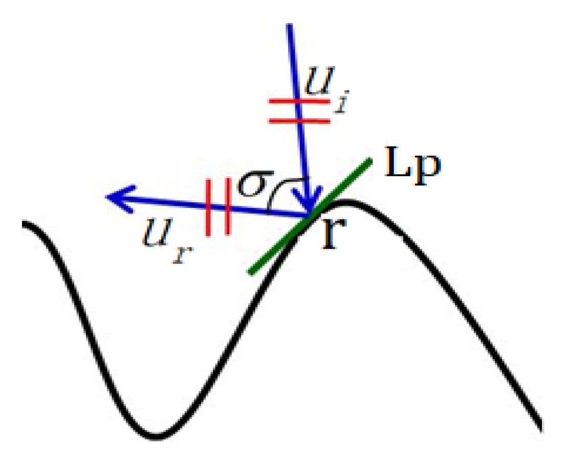
If $\delta m$ is considered a reflecting body that generates surface reflection, in order to describe the effect of the reflecting body boundary on the reflection and satisfy the need for imaging the boundary, this paper obtains the reflection wave general equation through the local reflection coefficient, defined as follows:

The directional derivative of $I_r$ along the incident wave propagation direction $I$ is defined as the local reflection coefficient of the local tangent plane on the reflecting body boundary, as Figure 2 shows:

$$r=\frac{\partial }{\partial I}\left(I_r\right).$$

(18)

In this equation, $r$ represents the local reflection coefficient of the local tangent plane at the reflecting body boundary location $x$. It can not only characterize the spatial position of the reflection surface but also reflect the property changes on the reflection surface. $I_r$, in mathematical form, is a step function, while $r$, in mathematical form, is a $\delta$ function distributed along the reflecting body boundary.

In Figure 2, $L_p$ is the local tangent plane at point $x$, $u_i$ and $u_r$ are the incident wave and the reflection wave with local plane wave properties.

Assuming that the seismic wavelength relative to the spatial variation characteristic scale of $m_b$ satisfies the high-frequency approximation condition, the incident wave propagation direction derivative in Definition (18) corresponds to $i{k}_i$ in the wavenumber domain, where $k_i$ is the wavenumber in the incident wave propagation direction, also known as the local wavenumber at $x$ position, as follows:

$$k_i=\frac{\omega }{v_b\left(x\right)}.$$

(19)

In this equation, $\omega$ is the circular frequency of the seismic wave and $v_b\left(x\right)$ is the velocity of the smooth model at position $x$. Therefore, Definition (18) in the high-frequency approximation has the following expression in the wavenumber domain:

$$r=i{k}_i{I}_r=\frac{i\omega }{v_b\left(x\right)}{I}_r.$$

(20)

The local reflection coefficient, defined by Equations (18) and (20), reflects the spatial variation in the relative perturbation of the subsurface physical parameters. In comparison with the reflection coefficient definition, Formula (8), given by Claerbout’s imaging condition in Section 2, the specular reflection coefficient is frequency-independent and dimensionless, while the local reflection coefficient is related to the propagation direction and has a dimension of reciprocal length. It is the reflection coefficient of a local plane incident wave acting on a local reflection plane under the high-frequency approximation, so it is related to the local wavenumber in the incident wave propagation direction (formally related to frequency).

Using the local reflection coefficient, Equations (14) and (15) can be rewritten as:

$$L\left(m_b\right)u_r=-\delta L_r\left(m_b,r,\sigma \right)u.$$

(21)

$$u_r=-{\displaystyle {\int }_{\mathrm{\Omega }}dvg{\ast }_t\delta L_r\left(m_b,r,\sigma \right)u}.$$

(22)

Similarly, when ignoring the multiple reflection waves, Equations (21) and (22) can be degenerated into the general wave equation for primary reflection waves based on the local reflection coefficient:

$$L\left(m_b\right)u_r=-\delta L_r\left(m_b,r,\sigma \right)u_i.$$

(23)

$$u_r=-{\displaystyle {\int }_{\mathrm{\Omega }}dvg{\ast }_t\delta L_r\left(m_b,r,\sigma \right)u_i}.$$

(24)

The difference between Equations (16) and (23) lies in $\delta L_r\left(m_b,I_r,\sigma \right)$ and $\delta L_r\left(m_b,r,\sigma \right)$. This difference leads to different inversion targets during migration. Equation (16) is based on wave impedance $I_r$, and its inversion target will be $I_r$ during migration, while Equation (23) is based on the local reflection coefficient $r$ defined by formula (18), and its inversion target will be $r$ during migration.

4. Theoretical Framework of the Seismic Data Waveform Imaging Method

According to the equations presented above for seismic wave propagation and Green’s function, we can obtain the following general linear integral representation for scattering data or reflection data:

$$u\left(x_{\mathrm{g}},t;x_s\right)={\displaystyle {\int }_{\mathrm{\Omega }}dxg\left(x_g,x,t\right){\ast }_{t}s\left(x,t;x_s\right)}.$$

(25)

Here, $s\left(x,t;x_s\right)$ is the virtual source term in Equations (12), (16), or (23), which contains $u_i\left(x,t;x_s\right)$, the model parameter, and the propagation operator.

Given $u\left(x_{\mathrm{g}},t;x_s\right)$ on the left side of Equation (25), estimating $s\left(x,t;x_s\right)$ on the right side corresponds to solving the first-class linear integral equation, also known as the inverse source problem. Discretizing Equation (25) into a matrix equation form, we obtain:

$$d=Lm.$$

(26)

In this equation, $d$ represents the common-shot gather seismic data matrix (i.e., primary scattering data or primary reflection data), $L$ represents the wavefield propagation matrix composed of wavefield propagation operators, and $m$ represents the subsurface virtual source matrix to be estimated.

For the matrix Equation (26), the following least squares solution can be obtained:

$$m={\left(L^{\ast }L\right)}^{-1}{L}^{\ast }d=L^{-g}d.$$

(27)

In this equation, $L^{-g}$ represents the least squares inverse matrix of the wavefield propagation matrix $L$, $L^{\ast }$ represents the adjoint matrix of matrix $L$. If $\left(L^{\ast }L\right)$ is a unitary matrix or the effect of ${\left(L^{\ast }L\right)}^{-1}$ is ignored, which means using $L^{\ast }$ as the inverse matrix of $L$, an approximate solution $m_a$ of the matrix, Equation (27), can be obtained as follows:

$$m_a=L^{\ast }d.$$

(28)

For large-scale inversion imaging, the least squares solution method of Formula (27) has difficulties and instability when calculating the inverse matrix, which can be solved through iterative methods, and the obtained solution has high fidelity and resolution.

The solution method of Formula (28) is also known as the back-projection method or back-propagation method. The calculation of $L^{\ast }$ in Formula (28) has little computational complexity and its stability is much better than calculating ${\left(L^{\ast }L\right)}^{-1}$ in Formula (27), but the fidelity and resolution of the obtained solution will be affected.

By solving Formula (27) or (28), an estimate of $s\left(x,t;x_s\right)$ can be obtained. In order to obtain the imaging result of $\frac{\delta m}{m_b}$, $I_r$, or $r$, it is necessary to calculate $u_i\left(x,t;x_s\right)$ using Equation (6) and then eliminate it from $s\left(x,t;x_s\right)$. At the same time, the specific forms of the scattering operator or reflection operator must also be considered and eliminated from $s\left(x,t;x_s\right)$.

Based on the above content, the following theoretical framework of the seismic data waveform imaging method can be obtained:

(1)

Use the observed seismic data to solve the inverse source problem and obtain an estimate of the subsurface scattering wave or reflection wave virtual source.

(2)

Use the wave Equation (7) with the smooth model to solve the subsurface incident wavefield.

(3)

Use the subsurface incident wavefield and the scattering or reflection operator to obtain imaging from the estimated solution of the scattering or reflection virtual source, including perturbations in the physical parameters, wave impedance, or local reflection coefficient for reflecting body boundaries.

When solving the inverse source problem within this theoretical framework, if the virtual source estimate is obtained using Formula (28), the corresponding waveform imaging method is called waveform migration (WFM). If the virtual source estimate is obtained using Formula (27), the corresponding waveform imaging method is called least-squares waveform migration (LSWFM).

5. Scalar Wave Scattering Data Waveform Imaging

If $m$ in the general wave, Equation (6), is only velocity $v\left(x\right)$, then Equation (6) is a non-homogeneous scalar wave equation:

$$\left[\frac{1}{v^2\left(x\right)}\frac{{\partial }^2}{\partial t^2}-{\nabla }^2\right]u\left(x,t;x_s\right)=f\left(t\right)\delta \left(x-x_s\right).$$

(29)

According to the perturbation method, for $u_i\left(x,t;x_s\right)$ in the smooth velocity model, we obtain:

$$\left[\frac{1}{{v_b}^2\left(x\right)}\frac{{\partial }^2}{\partial t^2}-{\nabla }^2\right]u_i\left(x,t;x_s\right)=f\left(t\right)\delta \left(x-x_s\right).$$

(30)

Assuming that $\delta v\left(x\right)$ satisfies the scattering body condition defined above, according to wave Equations (12) and (13), we can obtain the following scalar scattering wave equation:

$$\left[\frac{1}{{v_b}^2\left(x\right)}\frac{{\partial }^2}{\partial t^2}-{\nabla }^2\right]u_s\left(x,t;x_s\right)=\frac{a_v\left(x\right)}{v_b^2\left(x\right)}\frac{{\partial }^2{u}_i\left(x,t;x_s\right)}{\partial t^2}.$$

(31)

$$u_s\left(x_{\mathrm{g}},t;x_s\right)={\displaystyle {\int }_{\mathrm{\Omega }}dxg\left(x_g,x,t\right){\ast }_t\frac{a_v\left(x\right)}{v_b^2\left(x\right)}\frac{{\partial }^2{u}_i\left(x,t;x_s\right)}{\partial t^2}}.$$

(32)

In which $a_v\left(x\right)$ is the relative perturbation of velocity, with:

$$a_v\left(x\right)=1-\frac{v_b^2\left(x\right)}{v^2\left(x\right)}\approx \frac{2\delta v\left(x\right)}{v_b\left(x\right)}.$$

$u_s\left(x,t;x_s\right)$ represents the first-order scattering wave generated by $a_v\left(x\right)$. The right-hand term of Equation (31) is the virtual source generating the scattering wave, which contains the relative velocity perturbation, scattering operator, and incident wavefield. The scattering operator is composed of the smooth velocity model and the second-order time derivative; i.e., $\frac{1}{v_b^2\left(x\right)}\frac{{\partial }^2}{\partial t^2}$.

5.1. Scalar Wave Scattering Data Waveform Migration

Applying the above theoretical framework and its adjoint solution, Formula (28), to the linear integral, Equation (32), and after some simple derivation, we can obtain the following calculation formula for the approximate estimation of $a_v\left(x\right)$ in the scalar wave scattering data waveform migration.

(1)

The calculation of the subsurface incident wavefield:

$$\left[\frac{1}{{v_b}^2\left(x\right)}\frac{{\partial }^2}{\partial t^2}-{\nabla }^2\right]u_i\left(x,t;x_s\right)=f\left(t\right)\delta \left(x-x_s\right).$$

(33)

(2)

The approximate estimation of the subsurface scattering virtual source based on the boundary conditions and wavefield reverse-time propagation:

$$\left\{\begin{array}{c}\left[\frac{1}{{v_b}^2\left(x\right)}\frac{{\partial }^2}{\partial t^2}-{\nabla }^2\right]u_s\left(x,t;x_s\right)=0.\\ u_s\left(x,t;x_s\right)=u_s\left(x_g,t;x_s\right)\delta \left(x_g-x\right).\end{array}\right.$$

(34)

(3)

Obtaining the approximate estimation of $a_v\left(x\right)$:

$$a_v\left(x\right)=v_b^2\left(x\right){\displaystyle \underset{0}{\overset{T}{\int }}dt{u}_s\left(x,t;x_s\right)\frac{{\partial }^2{u}_i\left(x,t;x_s\right)}{\partial t^2}}.$$

(35)

As we approximate the scattering body as a point source body relative to the seismic wavelength, the approximate estimate of $a_v\left(x\right)$ obtained from Equation (35) can achieve the imaging of the spatial position of the scattering body [47,48,49].

The main difference between Formula (35) and the conventional reverse-time migration formula is the addition of the second-order time derivative. Therefore, the imaging result obtained is 180° phase-shifted (i.e., reverse polarity) relative to the conventional reverse-time migration result, and the resolution is also improved.

5.2. Scalar Wave Scattering Data Least Squares Waveform Migration

Based on the theoretical framework proposed above and the least squares solution in Formula (27), combined with the above scattering data waveform migration formula, we can obtain the iterative solution process of $a_v\left(x\right)$ for scattering data least squares waveform migration, as shown in Figure 3. The strategy applied in the flowchart is to reduce data residuals through iteration.

The calculation formulas for the specific process are as follows:

Initialization: let $k=0$, $a_v^k\left(x\right)=a_v^0\left(x\right)=0$, and use Formula (33) to calculate the incident wavefield.

Calculation formula for data residuals during iteration:

$$\delta d^k\left(x_g,t;x_s\right)=u_s\left(x_{\mathrm{g}},t;x_s\right)-{\displaystyle {\int }_{\mathrm{\Omega }}dxg\left(x_g,x,t\right){\ast }_t\frac{a_v^k\left(x\right)}{v_b^2\left(x\right)}\frac{{\partial }^2{u}_i\left(x,t;x_s\right)}{\partial t^2}}.$$

(36)

The reverse-time extrapolation of data residuals during iteration:

$$\left\{\begin{array}{c}\left[\frac{1}{{v_b}^2\left(x\right)}\frac{{\partial }^2}{\partial t^2}-{\nabla }^2\right]\delta u^k\left(x,t;x_s\right)=0.\\ \delta u^k\left(x,t;x_s\right)=\delta d^k\left(x_g,t;x_s\right)\delta \left(x_g-x\right).\end{array}\right.$$

(37)

Correction of $a_v^k\left(x\right)$ during iteration:

$$a_v^{k+1}\left(x\right)=a_v^k\left(x\right)+{\alpha }_k{v}_b^2\left(x\right){\displaystyle \underset{0}{\overset{T}{\int }}dt\delta u^k\left(x,t;x_s\right)\frac{{\partial }^2{u}_i\left(x,t;x_s\right)}{\partial t^2}}.$$

(38)

The ${\alpha }_k$ in correction Formula (38) is the iterative step size factor for the k-th iteration, which can be obtained via a simple linear search method or can be approximated through the bidirectional illumination intensity of seismic waves in the source direction and detector point direction [50,51,52,53,54,55,56].

6. Scalar Wave Reflection Data Waveform Imaging

In the given smooth velocity model, as the density change is not considered, the angle-related wave impedance relative perturbation is simplified to the angle-independent velocity relative perturbation; i.e., $I_r\left(x,\sigma \right)=a_v\left(x\right)$. Therefore, its imaging result is the same as in scalar wave scattering data waveform imaging. Therefore, we will focus on discussing the scalar wave reflection data waveform imaging based on the local reflection coefficient.

For the reflection generated based on the local reflection coefficient, as the density change is not considered, the angle-related local reflection coefficient is simplified to be angle-independent; i.e., $r\left(x,\sigma \right)=r\left(x\right)$. According to the linear forward representation of reflection described by the scalar wave equation, we have the following specific seismic wave propagation equation and reflection equation based on the local reflection coefficient:

$$\left[\frac{1}{{v_b}^2\left(x\right)}\frac{{\partial }^2}{\partial t^2}-{\nabla }^2\right]u_i\left(x,t;x_s\right)=f\left(t\right)\delta \left(x-x_s\right).$$

(39)

$$\left[\frac{1}{{v_b}^2\left(x\right)}\frac{{\partial }^2}{\partial t^2}-{\nabla }^2\right]u_r\left(x,t;x_s\right)=\frac{-r\left(x\right)}{v_b\left(x\right)}\frac{\partial u_i\left(x,t;x_s\right)}{\partial t}.$$

(40)

In which $r\left(x\right)$ is the directional derivative of the velocity relative perturbation along the incident wave propagation direction, with $r\left(x\right)=\frac{i\omega }{v_b\left(x\right)}{a}_v\left(x\right)$. The right-hand term of Equation (40) is the virtual source generating the reflection wave, containing the local reflection coefficient, reflection operator, and incident wavefield.

The corresponding reflection data integral expression is:

$$u_r\left(x_g,t;x_s\right)=-{\displaystyle {\int }_{\mathrm{\Omega }}dxg\left(x_g,x,t\right){\ast }_t\frac{r\left(x\right)}{v_b\left(x\right)}\frac{\partial u_i\left(x,t;x_s\right)}{\partial t}}.$$

(41)

6.1. Scalar Wave Reflection Data Waveform Migration

Applying the above theoretical framework and its adjoint solution Formula (28) to the linear integral Equation (41), after some simple derivation, the following calculation formulas for $r\left(x\right)$ in scalar wave reflection data waveform migration were obtained:

(1)

The calculation of the subsurface incident wavefield:

$$\left[\frac{1}{{v_b}^2\left(x\right)}\frac{{\partial }^2}{\partial t^2}-{\nabla }^2\right]u_i\left(x,t;x_s\right)=f\left(t\right)\delta \left(x-x_s\right).$$

(42)

(2)

The approximate estimation of the subsurface reflection virtual source based on the boundary conditions and wavefield reverse-time propagation:

$$\left\{\begin{array}{c}\left[\frac{1}{{v_b}^2\left(x\right)}\frac{{\partial }^2}{\partial t^2}-{\nabla }^2\right]u_r\left(x,t;x_s\right)=0.\\ u_r\left(x,t;x_s\right)=u_r\left(x_g,t;x_s\right)\delta \left(x_g-x\right).\end{array}\right.$$

(43)

(3)

Obtaining the approximate estimation of the velocity relative perturbation and the local reflection coefficient:

$$r\left(x\right)=-v_b\left(x\right){\displaystyle \underset{0}{\overset{T}{\int }}dt{u}_r\left(x,t;x_s\right)\frac{\partial u_i\left(x,t;x_s\right)}{\partial t}}.$$

(44)

The main difference between Formula (44) and the conventional reverse-time migration imaging formula is the addition of the first-order time derivative. Therefore, the imaging results obtained possess a phase difference of 90° relative to the conventional reverse-time migration result, and the resolution is also improved.

6.2. Scalar Wave Reflection Data Least Squares Waveform Migration

Similarly, we can obtain the iterative solution process of $r\left(x\right)$ for reflection data least squares waveform migration. The flowchart is similar to Figure 3 and is not repeated here.

The calculation formulas for the specific process are as follows.

Initialization: let $k=0$, $r^k\left(x\right)=r^0\left(x\right)=0$, and use Formula (42) to calculate the incident wavefield.

The calculation of data residuals during the iteration process for solving $r\left(x\right)$:

$$\delta d_r^k\left(x_g,t;x_s\right)=u_r\left(x_g,t;x_s\right)+{\displaystyle {\int }_{\mathrm{\Omega }}dxg\left(x_g,x,t\right){\ast }_t\frac{r^k\left(x\right)}{v_b\left(x\right)}\frac{\partial u_i\left(x,t;x_s\right)}{\partial t}}.$$

(45)

The reverse-time extrapolation of data residuals during the iteration process for solving $r\left(x\right)$:

$$\left\{\begin{array}{c}\left[\frac{1}{{v_b}^2\left(x\right)}\frac{{\partial }^2}{\partial t^2}-{\nabla }^2\right]\delta u_r^k\left(x,t;x_s\right)=0.\\ \delta u_r^k\left(x,t;x_s\right)=\delta d_r^k\left(x_g,t;x_s\right)\delta \left(x_g-x\right).\end{array}\right.$$

(46)

The correction of $r^k\left(x\right)$ during the iteration process:

$$r^{k+1}\left(x\right)=r^k\left(x\right)-{\alpha }_k{v}_b\left(x\right){\displaystyle \underset{0}{\overset{T}{\int }}dt\delta u_r^k\left(x,t;x_s\right)\frac{\partial u_i\left(x,t;x_s\right)}{\partial t}}.$$

(47)

7. Numerical Experiments

7.1. Sigsbee2A Model Numerical Experiment

The numerical experiment in this section uses the Sigsbee2A model data provided by SEG [57]. Figure 4a shows the stratigraphic model of Sigsbee2A. The model contains not only high-velocity salt bodies and fine strata but also many local high-velocity scattering bodies (red box in the figure) and horizontal high-velocity reflection surfaces at the bottom (blue box in the figure), making it suitable for verifying scattering data waveform migration and reflection data waveform migration. Figure 4b shows the velocity model for this migration experiment.

The model size is 1067 × 1201 grid points, with horizontal and vertical grid spacings of 22.86 m and 7.62 m, respectively. The observation system of these simulation data is the marine streamer observation system, with a total of 500 shots, shot spacing of 45.72 m, streamer length of 7932.42 m, detector point spacing of 22.86 m, varying numbers of traces per shot (minimum of 57, maximum of 348), time sampling interval of 8 ms, and 1500 time sampling points. The source wavelet is a Ricker wavelet with a dominant frequency of 25 Hz.

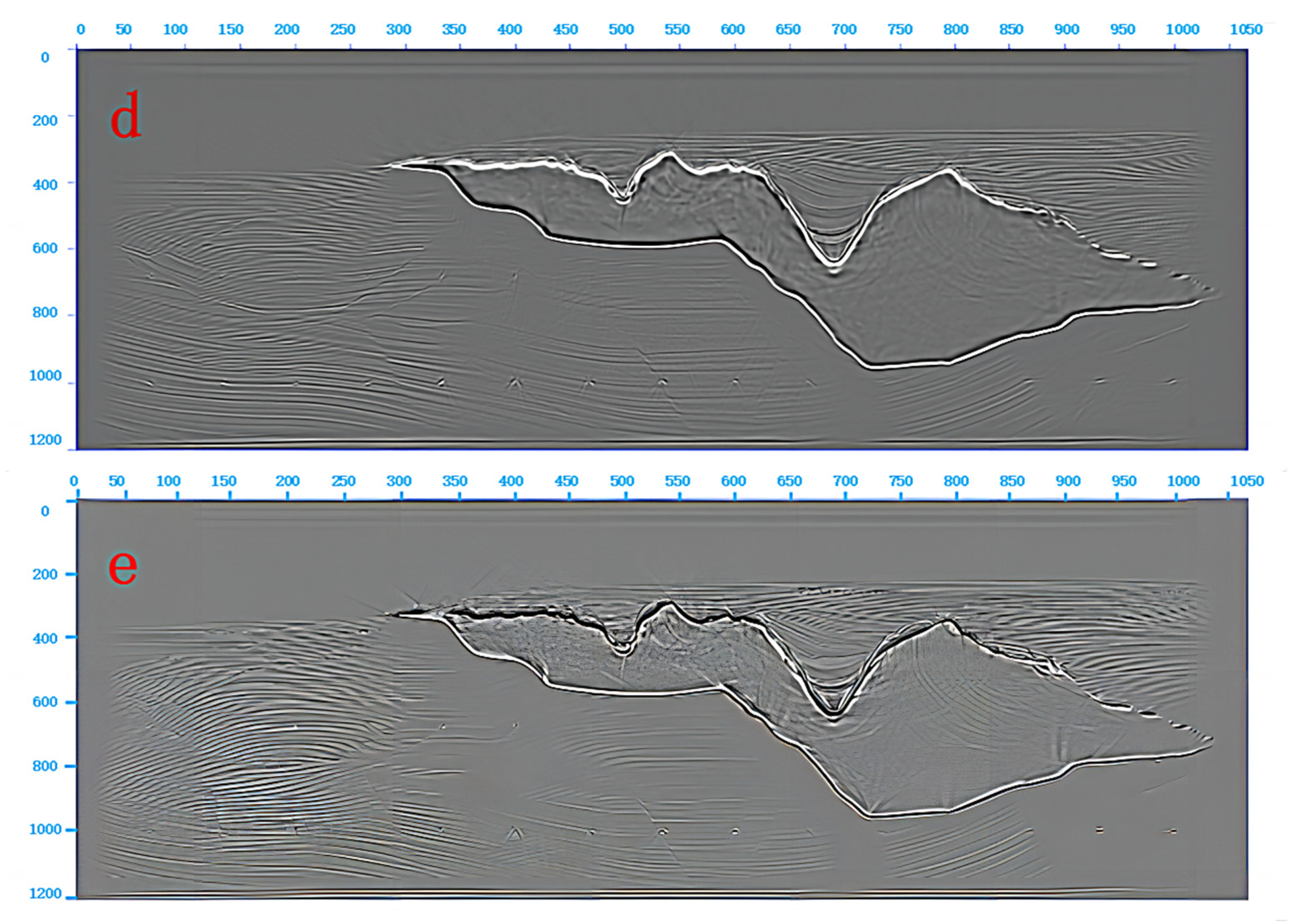
It is quite evident that the imaging results of the three migration methods are impressive. Through careful comparison, for the 15 high-velocity scattering bodies at the depth of 1000, Figure 4e shows the clearest and most delicate imaging among the three, but for high-velocity salt bodies and layered structures, Figure 4d shows the thinnest lines with the highest information content among the three. Therefore, for the imaging of the high-velocity scattering body, the scattering data WFM result is better than the other two. For the imaging of the reflection surfaces, the reflection data WFM result is better than the others.

To compare the differences in more detail, the migration results of the high-velocity scattering bodies shown by the red box and the high-velocity horizontal reflection surface shown by the blue box in Figure 4a are compared.

As can be seen from Figure 5, the scattering data WFM accurately images the high-velocity scattering body (imaging position and zero phase), the RTM accurately images the position of the high-velocity scattering body but has a 180° phase shift (reverse polarity), imaging the high-velocity scattering body as a low-velocity scattering body. The reflection data WFM result has a 90° phase shift in imaging the high-velocity scattering body, resulting in a shallower imaging position, with a depth error of one-quarter wavelength, and the high-velocity scattering body model is located in the middle of the transition zone from the wave peak to the wave trough in the imaging result. The amplitude spectra in Figure 5 also show that the resolution of the scattering data WFM result is higher than that of the RTM result, while the resolution of the reflection data WFM result is lower than the scattering data WFM result but higher than the RTM result. This indicates that the experimental results are consistent with the theory in this paper, and the time derivative of the incident wavefield is helpful for improving the resolution of the migration result.

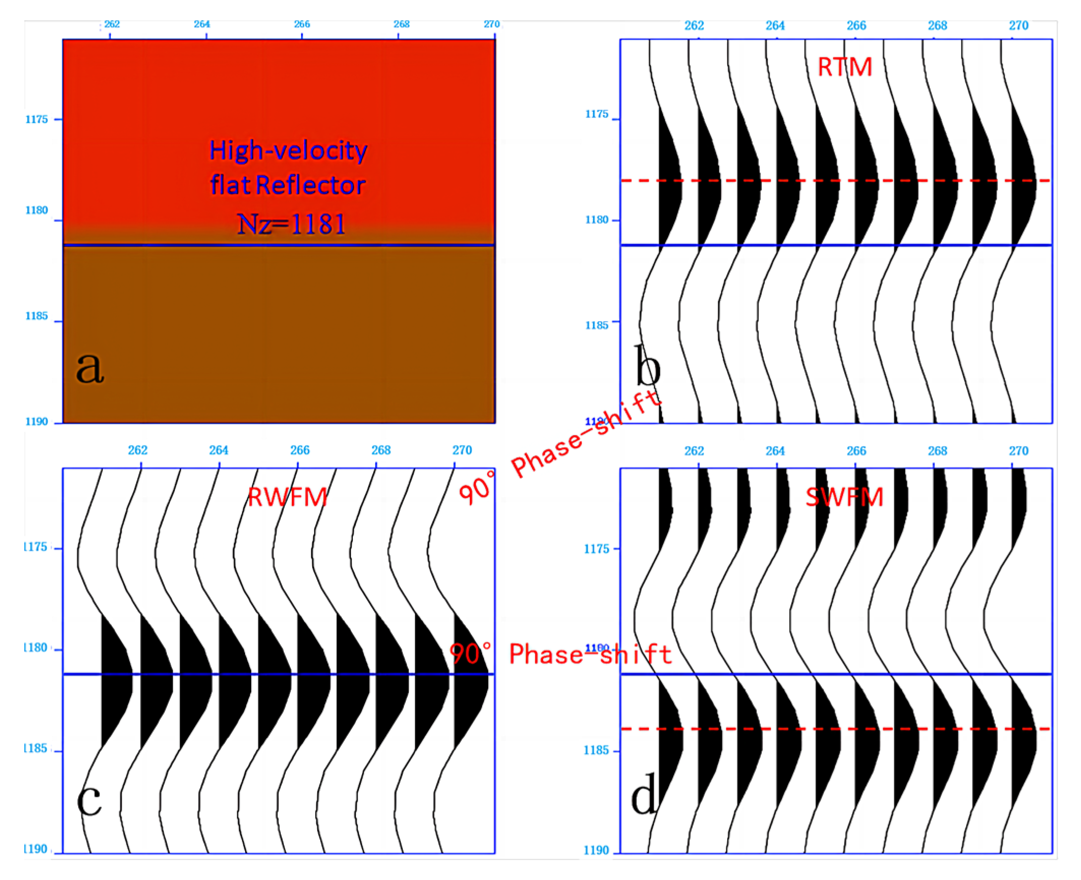
As can be seen from Figure 6, the reflection data WFM accurately images the position of the high-velocity horizontal reflection surface, while the RTM result has a phase shift of 90° in imaging the high-velocity horizontal reflection surface, resulting in a shallower imaging position, with a depth error of one-quarter wavelength, and the high-velocity horizontal reflection surface model is located in the middle of the transition zone from the wave peak to the wave trough. The scattering data WFM result has a −90° phase shift in imaging the high-velocity horizontal reflection surface, resulting in a deeper imaging position, with a depth error of one-quarter wavelength, and the high-velocity horizontal reflection surface model is located in the middle of the transition zone from the wave trough to the wave peak. This is consistent with the theory in this paper, and it is necessary to distinguish between scattering bodies and reflection bodies in the migration imaging process to obtain accurate and phase-correct migration results.

7.2. Marmousi Model Numerical Experiment

The internationally recognized standard model, the Marmousi model, was used for the numerical experiment. The velocity model used in this experiment is shown in Figure 7a. The model grid size is 343 × 750, with horizontal grid spacing of 25 m and vertical grid spacing of 4 m. The Marmousi model observation system is set as follows: a total of 240 shots, each shot has 96 receiving channels, shot spacing is 25 m, channel spacing is 25 m, the first shot ground position is 2575 m, recording length is 3 s, time sampling rate is 4 ms, and the source wavelet is a Ricker wavelet with a dominant frequency of 25 Hz.

The three methods are applied to the Marmousi model data to obtain the migration results shown above. As observed, all three achieve relatively satisfying imaging results. Through careful comparison, it was found that Figure 7d has the thinnest lines and the most delicate imaging quality, and the small-scale layered structures in it is much clearer than the other two, while Figure 7b has thicker lines but provides more complete and clear information in the imaging of reflection surfaces. The conventional RTM results have the thickest lines. Therefore, the scattering WFM result excels in resolution, followed by the reflection data WFM, and the conventional RTM exhibits the lowest level of resolution. Thus, the proposed waveform migration can effectively improve the resolution of the imaging results.

Furthermore, by observing the phase of the scattering WFM result and the conventional RTM imaging result, it can be seen that the two have opposite phases, with a 180° phase difference, which is consistent with the theory in this paper.

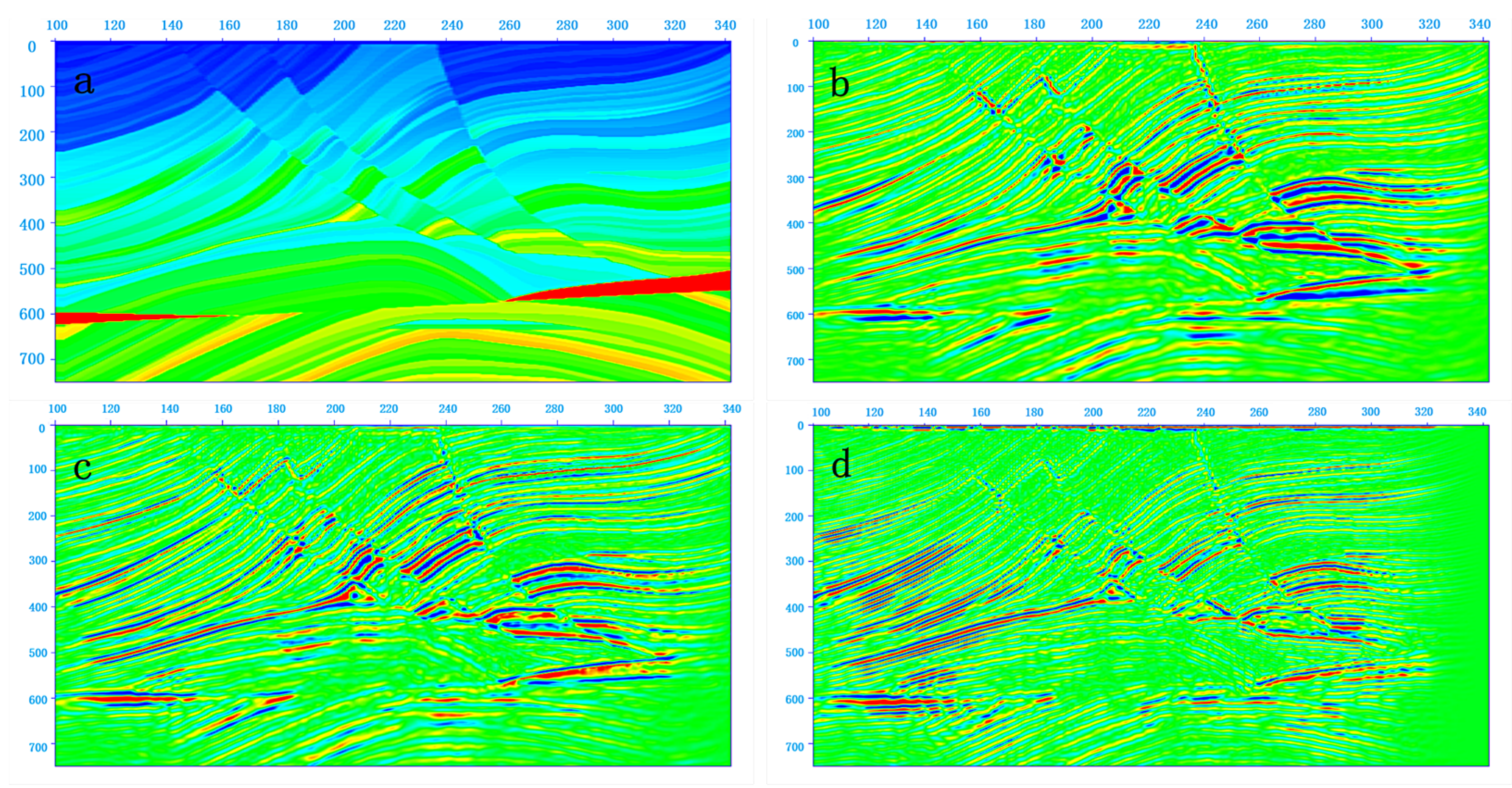
7.3. Scalar Wave Reflection Data Least Squares Waveform Migration Numerical Experiment

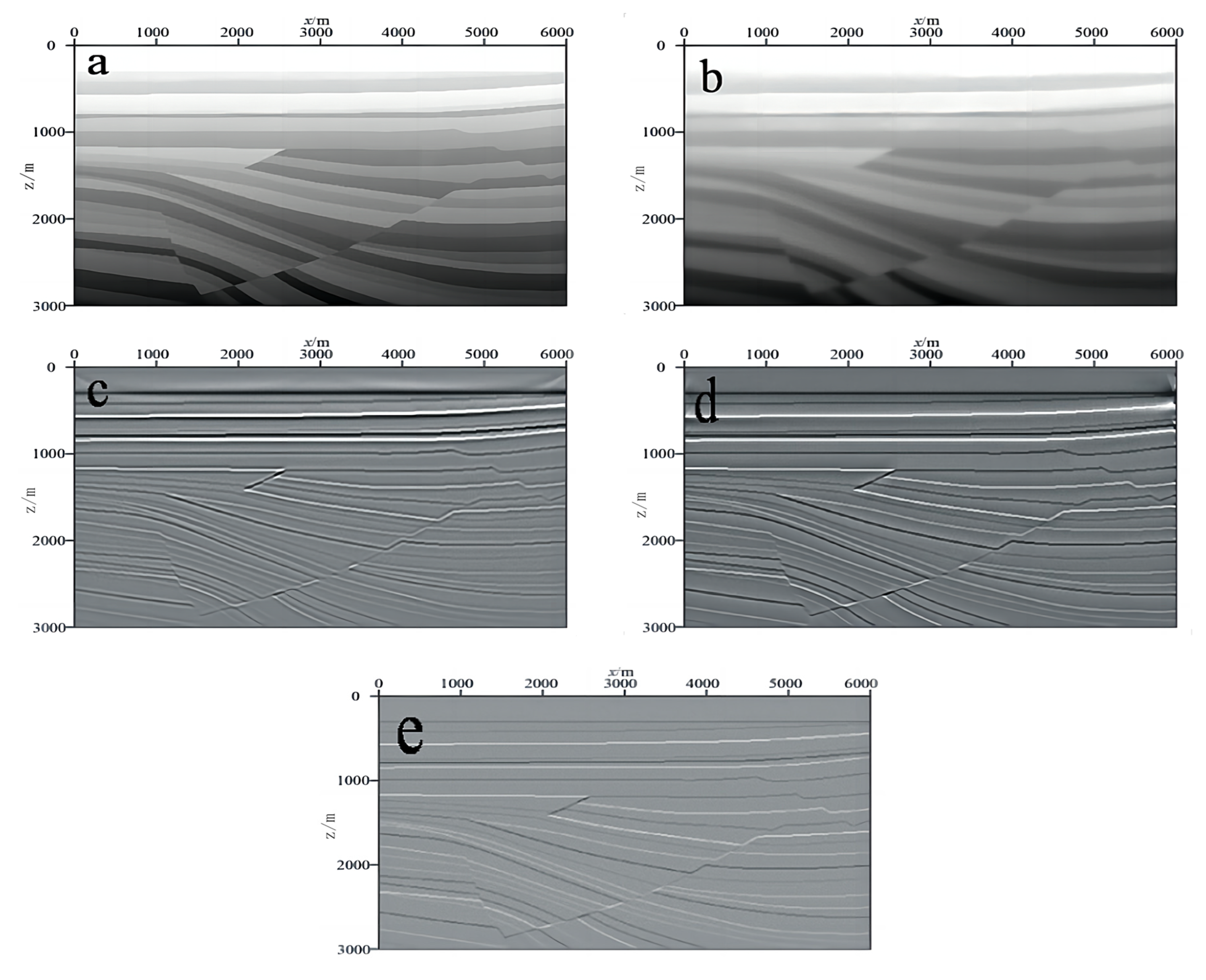
To verify the reflection data least squares waveform migration based on the local reflection coefficient proposed in this paper, we take a part of the Sigsbee2A velocity model for the experiment.

For the velocity model in Figure 8a, seismic data are synthesized using the finite difference method of the scalar wave equation. In this experiment, 300 shot seismic data are synthesized, with shot points ranging between 0 km and 6 km, shot spacing of 20 m, middle shot with receiving on both sides, 601 channels per shot, channel spacing of 10 m, time sampling interval of 0.5 ms, 3000 time sampling points, and a Ricker wavelet source with a dominant frequency of 18 Hz. As the velocity model in Figure 8a has a layered structure, the synthesized seismic data are mainly reflection data.

In the experiment, we first applied the proposed reflection data WFM based on the local reflection coefficient to the synthesized shot gathering data. Figure 8d shows the migration result with a total of 35 iterations performed. To more intuitively show the advantage of fidelity in the LSWFM results, the true vertical reflectivity of the model is shown in Figure 8e.

As can be seen from Figure 8c, the reflection data WFM based on the local reflection coefficient can obtain good imaging results for this model. By further comparing Figure 8c,d, the lines of the layer interfaces and fault surfaces in Figure 8d are clearer, and display more information about the layered structures. Thus, the resolution of the LSWFM result is significantly improved. Compared with Figure 8e, the amplitude fidelity of the LSWFM result is also significantly improved.

8. Conclusions

Based on a detailed study of the current seismic wave equation migration imaging methods, through theoretical derivation and experimental verification, this paper outlines the following conclusions.

(1)

We suggest dividing the heterogeneous body into scattering bodies generating waves with finite spatial extension and reflecting bodies generating waves with a specific spatial extension. By considering reflecting bodies and reflection waves as high-frequency approximations of scattering bodies and scattering waves, we can view subsurface virtual sources generating reflection waves as local plane wave sources integrated from point sources, and the generated reflection waves as directional local plane waves, distinct from scattering waves.

(2)

We propose a correction to the reflection coefficient in the current migration imaging formula, which can only describe the plane wave with a small angle incident on the infinitely flat reflection interface. For the reflecting body and reflection wave, the directional derivative of the wave impedance relative perturbation along the direction of the incident wave propagation is defined as the local reflection coefficient on the reflecting body boundary. Meanwhile, a linear forward representation for seismic primary reflection data based on the local reflection coefficient is obtained.

(3)

Based on the linear forward representations for seismic data, this paper uses linear inversion theory to establish a theoretical framework of seismic data waveform imaging facing scattering data and reflection data separately. Scattering data waveform imaging is a linear inversion of scattering body physical parameter perturbations. Reflection data waveform imaging is a linear inversion of reflecting body wave impedance relative to the perturbation or local reflection coefficient, which can not only achieve the accurate imaging of reflection interface positions but can also obtain the lithology imaging of formation wave impedance relative changes.

(4)

Within the theoretical framework of waveform imaging, this paper uses the adjoint operator and least squares inverse operator to perform the backward propagation of seismic waves, degrading waveform imaging into WFM and LSWFM. WFM has a small computational load and good stability, but its migration imaging result has insufficient fidelity and resolution. LSWFM has a large computational load, but its migration imaging result has good fidelity and a high resolution. Compared with the conventional RTM and LSRTM, WFM and LSWFM only add the calculation of the time derivative of the incident wavefield; therefore, the computational load does not increase on a comparative basis.

This proposed method, both theoretically and experimentally, is limited to 2-D models and combines with scalar waves. We hope to extend it to 3-D models combined with acoustic or elastic wave equations on the existing basis, which is also the direction of the next research project.