Article

A Comparative Study of the Driving Factors of Water Resources Use Efficiency in China’s Agricultural and Industrial Sectors

College of Economics and Management, China Three Gorges University, Yichang 443002, China
*
Author to whom correspondence should be addressed.
Water 2024, 16(3), 387; https://doi.org/10.3390/w16030387
Submission received: 21 December 2023 / Revised: 21 January 2024 / Accepted: 22 January 2024 / Published: 24 January 2024
(This article belongs to the Special Issue Water Sustainability and High-Quality Economic Development)

Abstract

:
The efficient use of water resources has become an important topic in China. Research on measurement and driving factors is the foundation for improving water resources use efficiency (WRUE). In this paper, the super-efficiency slacks-based measure (SE-SBM) model is used to measure the WRUE of China from 2005 to 2021. The agricultural carbon emissions and chemical oxygen demand (COD) in industrial wastes are taken as undesirable by-products. The driving factors of WRUE are discussed with use of the Tobit regression model. The results show that China’s agricultural WRUE ranges from 1.185 in Jilin to 0.687 in Ningxia. In the industrial sector, the WRUE ranges from 1.399 in Beijing to Jiangxi 0.212. The economic structure and development level, water resources endowment, government influence and environmental regulation, agricultural planting scale and urbanization rate have impacts on WRUE. Precautionary measures need to be applied to prevent inefficient WRUE caused by the declining share of the industrial sector in the economic structure. More financial support should be focused on water-saving irrigation in agriculture and energy and resource efficiency in industry. The organizational structure and technological advantages of urbanization should also be emphasized in efforts to improve water efficiency.

1. Introduction

Water resources are important natural and strategic economic resources that underpin the survival and development of human societies [1,2]. Under the challenge of climate change, water scarcity has become a growing problem [3,4]. By 2025, approximately two-thirds of the population will have to live under water-stressed conditions. Water resources use efficiency (WRUE) is a crucial indicator of the sustainability of an economy [5,6]. Therefore, comprehensively improving WRUE is an urgent priority to address the prominent imbalance between water supply and demand [7]. Governments are encouraging efficiency measures to conserve water resources [8]. So, the sustainable development of water resources and green and high-quality economic development are promoted [9].
The total water resources of China in 2022 were 2708.81 billion m3, ranking fourth in the world [10]. However, the per capita water resources possession is only one quarter of the world level, making China one of the 13 countries with the poorest water resources in the world [7,11]. China is currently in a critical stage of industrialization and modernization. However, the rough economic development of the past decades has led to low WRUE in China. Water scarcity is particularly pronounced [12,13]. Research on the measurement and driving factors of WRUE is the foundation for improving [14], which would provide the support for alleviating water scarcity.
There are various methods to measure WRUE. The parametric approach represented by stochastic frontier analysis (SFA) [15,16] and the non-parametric approach typified by data envelopment analysis (DEA) are the dominant methods. There is a complex interaction between the environment and the production process during the use and treatment of water resources. It is difficult to apply an explicit functional form to evaluate the WRUE by parametric methods. Therefore, non-parametric methods were introduced to measure WRUE. The super-efficiency DEA model [17], three-stage DEA model [18], slacks-based measure (SBM) model [19], undesirable output super efficiency slacks-based measure (SE-SBM) model [20], network DEA model [21], and other various DEA improvement methods have been developed. In the spatial dimension, WRUE has been measured at the urban [22], provincial [23,24], basin [19,25], and national [21,26] levels. Scholars have evaluated WRUE in different water use sectors of agriculture, industry, the domestic sphere, and ecology. Huang et al. [27] evaluated the efficiency of the plantation, forestry, animal husbandry, and fishery industries, concluding that China’s overall agricultural WRUE has shown a fluctuating downward trend. Shi et al. [28] and Qi and Song [29] evaluated the WRUE of the Yangtze River Economic Belt for agriculture and industry, respectively.
The literature has also explored the drivers of WRUE changes from natural, economic, and social perspectives. Yu and Liu [30] concluded that WRUE is negatively correlated with investment in wastewater treatment projects and industrial water use structure, and positively correlated with the total amount of water supplied and the level of science and technology. Ma et al. [31] concluded that the technological progress has a positive impact on WRUE, whereas water costs and environmental pollution reduced the efficiency. For the factors affecting agricultural WRUE, researchers have focused on resource endowment [32], industrial structure [33], soil type [34], water conservancy facilities [35], and the agricultural planting structure [36]. The driving factors of industrial WRUE have been studied. Cheng and Zhang [37] argued that the water price is an important factor influencing industrial WRUE. He et al. [38] explored the impact of variables such as per capita gross domestic product (GDP), per capita water consumption, the proportion of secondary and tertiary industry water use, foreign direct investment, and research & development (R&D) intensity. Furthermore, scholars have also looked at the influence of environmental regulation [39], population density [22], and government policy [29].
These studies have provided evidence on the measurement and driving factors of WRUE. However, there are still some gaps in the research. On the one hand, the measurements of WRUE have focused on desirable outputs. The attention paid to undesirable outputs such as pollution emissions from industrial and agricultural production has been limited. As environmental issues are gradually being paid attention to, adding appropriate environmental indicators as undesirable outputs will undoubtedly make the measurement results reasonable. On the other hand, most studies have analyzed WRUE in society as a whole, or have focused on only one of the industrial or agricultural sectors in isolation. This makes comparative analysis between the agricultural and industrial sectors difficult. Neglecting undesirable outputs makes the study results invalid for supporting cleaner production and sustainability. The lack of comparative analysis will also make policy implications incompatible with both the agricultural and industrial sectors.
Therefore, this paper adopts the SE-SBM model with the undesirable outputs to measure WRUE in agriculture and industry in 31 provinces or cities in China. Then, Tobit regression is applied to investigate the driving factors in different water use sectors. For the first time, a comparative discussion is conducted on the driving factors of agricultural and industrial WRUE. The foundation for water management policy development from a comprehensive agriculture–industry perspective is provided.
The rest of the paper is organized as follows. Section 2 introduces the research methods and materials. Section 3 presents the results. Section 4 discusses the empirical results. Finally, Section 5 summarizes the main conclusions and proposes policy implications.

2. Methods and Materials

2.1. Research Methods

2.1.1. SE-SBM Model

The SBM model was originally proposed by Tone [40]. It is a non-radial and non-angular data envelopment analysis method. However, when multiple decision-making units (DMUs) are evaluated as effective in the SBM, the efficiency level of effective DMUs cannot be further distinguished. Andersen and Petersen proposed the super-efficiency model to resolve this [41]. Besides the outputs defined as “good” such as GDP, there are also “bad” or “undesirable” outputs such as wastewater, exhaust, and solid waste. Based on this, Tone [42] further proposed the SE-SBM model of undesirable outputs, which could comprehensively consider the relationship between inputs, outputs, and pollution. Therefore, an undesirable output-oriented SE-SBM model was selected to measure the WRUE.
The undesirable output SE-SBM model of water resources uses efficiency as follows [42]: In Equation (1), the objective function W is the efficiency value of the decision unit, i.e., the WRUE of each region in this paper; x i j is the input i of the DMU j ; y r j is the output r of the DMUs j ; s i , s r g + , s t b are the slack variables of the inputs, desirable outputs, and undesirable outputs, respectively; λ is the vector of weights. For a decision-making unit, it is valid if and only if its value is 1, i.e., it satisfies the equality of s , s g , and s b . Otherwise, the decision-making unit is invalid or has efficiency losses.
M i n W = 1 + 1 m i = 1 m s i - x i k 1 - 1 q 1 + q 2 r = 1 q 1 s r g + y r k g + t = 1 q 2 s t b - y t k b
s . t . j = 1 , j k n x i j λ j s i x i k j = 1 , j k n y r j g λ j + s r g + y r k g j = 1 , j k n y t j b λ j s t b - y t k b 1 - 1 q 1 + q 2 r = 1 q 1 s r g + y r k g + t = 1 q 2 s t b - y t k b > 0 s > 0 , s g > 0 , s b > 0 , λ > 0 i = 1 , 2 , , m ; r = 1 , 2 , , q ; j = 1 , 2 , , n ( j k )

2.1.2. Tobit Regression Model

The Tobit model is a standard censored model. Tobit differs from discrete variable models or continuous variable models in that the dependent variable is restricted and consists of two types of equations. The efficiency obtained by the DEA model is affected by the input and output indicators and other environmental factors such as the regional economic level, labour market, and financial support [43]. The estimation of linear regression in the presence of censoring includes additional computational complications. The ordinary least squares regression produces inconsistent parameter estimates because the censored samples are not representative of the total. The values of the SE-SBM model measured in this paper are truncated data greater than 0. Therefore, the Tobit model is appropriate for exploring the drivers of WRUE.
The general form of the Tobit model is Equation (2) [44]. The negative values of the explanatory variable y i are replaced by 0. The bias brought by the regression reduced.
y i = β x i + u i
The model (2) can be transformed to:
W R U E i t = c + β 1 X 1 + β 2 X 2 + + β i X i + + β 9 X 9 + ε i t ( i = 1 , 2 , , 9 )
where W R U E i t is the WRUE considering undesirable outputs, i , t denote the values for different regions in different time periods, X i ( i = 1 , 2 , , 9 ) are independent variables, which will be explained in detail below; β i ( i = 1 , 2 , , 9 ) denote the coefficients to be estimated for the variables of interest; ε is the random error.

2.2. Variable Selection and Data

2.2.1. WRUE Measurement Variables

Measurement variables should be able to effectively reflect the economic, social and environmental impacts of water use. Regarding the input–output relationship of water resources use in the process of economic growth, Jorgenson and Stiroh [45] proposed the KLEM (capital, labor, energy, and materials) model. The KLEM model decomposes inputs into capital, labor, energy, and intermediate inputs, and outputs refer to desirable outputs of economic significance. While obtaining agricultural and industrial products, some undesirable by-outputs cannot be avoided. Referring to literature, the input–output index system is constructed.
(1)
Agricultural sector
In agricultural production, inputs such as land, labor, and capital are indispensable. However, the carbon emissions that come with receiving crops are undesirable but objective. The rural population, amount of agricultural fertilizer (in tons), total power of agricultural machinery (in kilowatts), agricultural water consumption (m3), and the effective irrigated area (hectares) are selected as the input indicators. The real GDP of agricultural output (in CNY) and the grain yield (tons) are the desirable output indicators. The undesirable output is agricultural carbon emissions (tons) [20,31,46] (Table 1).
(2)
Industrial sector
Similarly, the number of employees, capital stock (CNY), and industrial water consumption (m3) are selected as input variables. The real GDP (CNY) and chemical oxygen demand (COD) emissions (ton) from wastewater are selected as desirable outputs and undesirable outputs, respectively (Table 2).

2.2.2. Tobit Regression Variables

Based on previous research and referring to the literature [20,31,46], the driving factors of WRUE are considered from the following aspects: (1) industrial structure: primary industrial proportion (%) and secondary industrial proportion (%); (2) economic level: per capita GDP (CNY); (3) water resources: water resources endowment (m3), groundwater proportion (%), utilization rate of water (%), and industrial water proportion (%); (4) influence of the government: financial support (proportion of regional financial expenditure on science and technology, %) and R&D intensity (proportion of R&D expenditure to GDP, %); (5) environmental protection: environmental regulation (proportion of completed investment in pollution control to GDP, %); (6) in the agricultural sector: the agricultural planting area (hectares) are added; (7) in the industrial sector: the urbanization rate (%) is added. The definitions and descriptions of variables are shown in Table 3, Table 4 and Table 5. Given the existence of ratio-type variables and numerical variables in factors, to make the data comparable, the numerical data are firstly logarithmically processed.

2.2.3. Data

The data are obtained from the China Statistical Yearbook and the statistical yearbooks published by the official of the regional statistical bureaus. The economic-related data are all processed with 2005 as the base period.
The data on agricultural carbon emissions are calculated by combining the methodology in the recommended guidelines of the Intergovernmental Panel on Climate Change (IPCC) and the study of Hu et al. [47]. The capital stock data of the secondary industry are calculated by the “perpetual inventory method” mentioned by Zhang et al. [48].

3. Results

Inter-provincial WRUE from 2005 to 2021 in China was measured with the SE-SBM model. The WRUE of the agricultural and industrial sectors was also measured separately. The WRUE results for the industrial sector are up to 2020.

3.1. WRUE Measurement Results

3.1.1. Overall Results of WRUE in China

The WRUE results are shown in Table 6. Given the space limitation, not all results up to 2015 have been listed. The average inter-provincial WRUE in China ranges from 1.156 in Beijing, the highest, to 0.501 in Ningxia, the lowest. In Beijing, Tianjin, Shanghai, and Guangdong, some WRUE values are greater than 1. This is a further distinction of the efficiency level of effective DMUs when they are evaluated as effective in the SBM. This is the advantage of “super-efficiency” in the SE-SBM.

3.1.2. Agricultural WRUE

The agricultural WRUE results are shown in Table 7 and Figure 1.
The mean value of agricultural WRUE in China was above 0.9 from 2005 to 2021. The highest value was Jilin (1.185), indicating that Jilin was better matched in terms of fertilizers, machinery, labor, and water resources. The lowest mean value was Ningxia (0.687), which is in the arid inland areas of Northwestern China. The inefficiency indicates the mismatch between agricultural activities in economic layout and water use [49].

3.1.3. Industrial WRUE

The industrial WRUE results are shown in Table 8 and Figure 2.
In the industrial sector, WRUE ranges from the highest of 1.399 in Beijing to the lowest of 0.212 in Jiangxi. The average WRUE is 0.429 during 2005–2020 in the industrial sector, with a declining trend. This suggests that China’s rapid economic growth over the period was based on low industrial WRUE. There was an average annual decrease of 4.16% from 2005 to 2010 and 1.84% after 2011. The slowdown in efficiency reduction is indicative of China’s sustainable development efforts.

3.2. Driving Factors

The results of Tobit regression are shown in Table 9, Table 10 and Table 11.
The overall driving factors result of WRUE in China (Table 9).
Table 9. Tobit regression result of driving factors in China.
XVariable NameRegression CoefficientStandard Deviation
X1Tertiary industrial proportion−0.000850.0039398
X2Level of opening up−0.01738210.0477747
X3Economic level 0.3056228 ***0.0984446
X4Water resources endowment−0.0340230.0338003
X5Agricultural water proportion−0.0141513 ***0.0032433
X6Population−0.1791625 **0.083117
X7Urbanization rate−0.017255 **0.0070058
X8Financial support0.0650491 **0.0294161
CConstant term1.271306 *0.7247596
Note: *, **, *** indicate significant at the 10%, 5% and 1% levels, respectively.
The WRUE driving factors result in agricultural sector (Table 10).
Table 10. Tobit regression result of driving factors in agricultural sector.
XVariable NameRegression CoefficientStandard Deviation
X1Primary industrial proportion−0.00071420.0019784
X2Secondary industrial proportion −0.0050987 ***0.0006222
X3Economic level 0.01752120.0113597
X4Water resources endowment−0.00493760.0091182
X5Groundwater proportion−0.1183793 *0.0671602
X6Effective irrigated area−0.1469869 ***0.0260604
X7Agricultural planting area 0.1446299 ***0.0202212
X8Financial support−0.0040641 **0.0017402
X9Environmental regulation−0.0270033 ***0.0098143
CConstant term1.041346 ***0.1827509
Note: *, **, *** indicate significant at the 10%, 5% and 1% levels, respectively.
The WRUE driving factors result in industrial sector (Table 11).
Table 11. Tobit regression result of driving factors in industrial sector.
XVariable NameRegression CoefficientStandard Deviation
X1Primary industrial proportion−0.00133460.0025046
X2Secondary industrial proportion0.0036085 ***0.0009079
X3Economic level−0.0724771 ***0.0198431
X4Water resources endowment−0.01522940.014615
X5Utilization rate of water−0.0002677 ***0.000101
X6Industrial water proportion−0.0040386 ***0.0011027
X7Urbanization rate0.003648 **0.0016135
X8R&D intensity−0.0415154 ***0.0146881
X9Environmental regulation−0.00861810.0113406
CConstant term1.124456 ***0.2088492
Note: **, *** indicate significant at the 5% and 1% levels, respectively.

4. Discussion

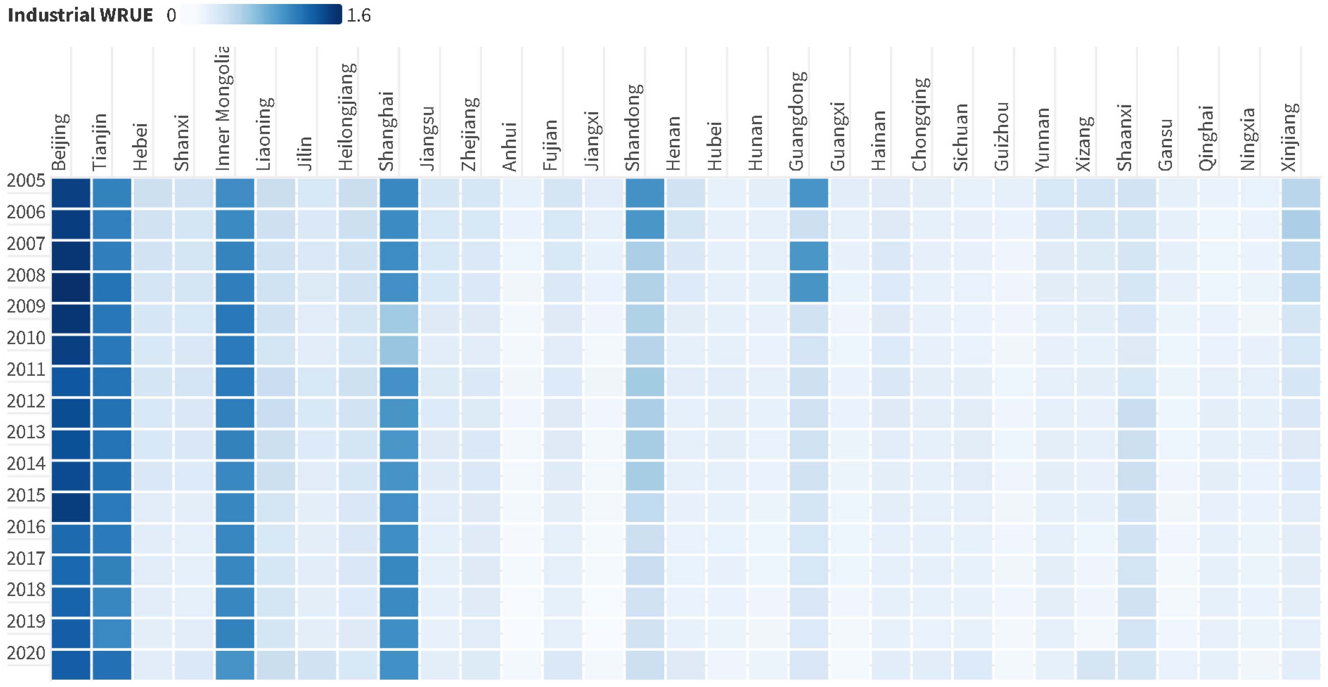
In the agricultural sector, the average WRUE reached over 1.0 in Beijing, Shanghai, Hainan, Heilongjiang, Jilin and Liaoning. As in the industrial sector, developed provinces and cities pay more attention to urban pollution and resource intensification issues. Therefore, the industrial WRUE of such provinces as Beijing, Tianjin, and Shanghai is basically above 1.0. In the less developed regions, there is still a need for water-intensive enterprises to promote economic growth. The industrial WRUE in these regions has been made to be inefficient, with all of them below 0.3.
Based on the Tobit regression results, the driving factors of WRUE change are discussed as follows.

4.1. Economic Structure and Level

The share of the industrial sector is significantly negatively correlated with water efficiency in agriculture, and positively correlated with industrial water efficiency. The regression coefficients are −0.0050987 and 0.0036085, respectively. An increase in the share of the industrial sector usually means a lower share of agriculture in GDP and better economic development. This confirms that the scale effect also exists in the efficient use of industrial water. Whereas, as a whole, the level of economic development positively drives WRUE. The agglomeration effect of industry, higher levels of management and technology, better water protection policies, and infrastructure investments in wastewater treatment all contribute to efficiency.
The negative relationship with the coefficient of −0.0724771 between the economic level and industrial WRUE deserves attention. This may be attributed to the fact that with the economy developing, the share of the tertiary sector increases and the weight of industry decreases. The reduction in the size of industry makes the sector less efficient in water use, which is also in line with the previous scale effect. There is no doubt that economic development is conducive to the efficient use of water. However, in the economic growth driven by the tertiary sector, the problem of declining industrial water efficiency cannot be ignored.

4.2. Water Resources Endowment

Water resources endowment is negatively correlated with WRUE in both agriculture (−0.0049376) and industry (−0.0152294) with P not being significant at 10% (0.31 in the whole, 0.58 in agriculture, 0.29 in industry). This suggests an underlying tendency for water scarcity areas to use water more efficiently than water-abundant areas. The proportion of groundwater in total water consumption is significantly negatively correlated (−0.1183793) with agricultural WRUE.
A high share of groundwater use in agricultural production usually implies a poor water endowment. It means that results, after taking into account for agricultural carbon emissions, provide evidence to the contrary. In other words, after accounting for agricultural carbon emissions, agricultural water efficiency in water-scarce areas will be lower than in water-abundant areas.
Similarly, in industry, the higher the proportion of water resources exploited is, the poorer will be the water endowment. At this point, the industrial WRUE after considering the industrial COD emissions is lower in water-scarce areas.
This is a result that diverges from common sense and previous research. This result indicates that the relationship between water resources endowment and WRUE needs to be further studied, given that climate change and environmental protection are increasingly concerned [50].

4.3. Government Influence and Environmental Regulations

Government financial support positively (0.0650491) promotes the overall WRUE. However, the negative (−0.0040641) impact of government investment in agriculture, forestry and water affairs on agricultural WRUE is of great concern. The maintenance and construction of new water conservancy facilities are believed to improve the efficiency of irrigation water use [51]. This view is challenged by the negative impact of government financial support for agriculture on WRUE. This becomes reasonable when the focus of financial support is on ensuring the total water supply and output in agriculture, rather than on water-saving facilities. Government financial support for agriculture should raise the concern for agricultural water conservancy in order to avoid excessive waste of precious water resources and improve water efficiency. A similar situation also occurs in the industrial sector. The increase in R&D intensity reduces industrial WRUE. It shows that the focus of R&D is not on energy conservation and resource efficiency, but on other aspects. This coincides with the fact that China’s industry has not yet reached the stage of high-quality development. Whether it is agriculture or industry, on the path of green and sustainable development, financial support should encourage more efficient use of resources.
Unsurprisingly, environmental regulations have had a negative impact (−0.0270033 in agriculture, −0.0086181 in industry) on water efficiency [52]. The reason is clear: environmental protection has increased the cost of production. However, this is not a reason to relax environmental regulations. On the contrary, it confirms that government financial support should increase investment in the green ecological development of agriculture and industry.

4.4. Non-Shared Factors between Agriculture & Industry

In the agricultural sector, the effective irrigation area and the sown area of grain crops have a negative (−0.1469869) and positive (0.1446299) impact on agricultural water resources, respectively. It is clear that more sown area of grain crops will increase agricultural water use. However, the scale effect of agricultural cultivation has improved WRUE. The effective irrigation area is also closely related to agricultural water consumption. More agricultural water use leads to a decrease in efficiency, confirming low irrigation efficiency in China. This is consistent with China’s low level of water-saving irrigation construction. Promoting water-saving irrigation is an important way to improve the WRUE in the agricultural sector.
The urbanization rate and industrial WRUE are significantly positively correlated, with a coefficient of 0.00364. China’s urbanization rate rose from 43.0% to 64.7% between 2005 and 2021. The high urbanization rate has led to a rapid increase in the total amount of domestic and industrial water use, accompanied by increasing industrial WRUE [53]. The positive relationship indicates that high urbanization rates have been able to eliminate negative impacts through organizational coordination and technological progress. It shows that China’s urbanization construction is in the stage of high-quality. Organizational advantages and scientific and technological means have been utilized to achieve ecological and green development of efficient use of resources.

5. Conclusions

This paper firstly measures the WRUE of agriculture and industry in China with the SE-SBM model, considering agricultural carbon emissions and industrial pollution as undesirable outputs. Then, the Tobit regression is applied to discuss the driving factors of WRUE in the agricultural and industrial sectors.
The main conclusions are as follows: (1) Economic development is conducive to the improvement of overall WRUE. The higher the proportion of industry there is in the economy, the higher will be the industrial WRUE. There is a scale effect in industrial WRUE. When the proportion of the tertiary industry in the economic structure increases and the industrial proportion decreases, the WRUE will be negatively affected. (2) The agricultural WRUE of the areas with poor water endowment is lower than that of the areas with abundant water resources. Similarly, industrial WRUE in water-scarce areas is lower than that in water-rich areas. Today, ecological development has received great attention and the relationship between water resources endowment and WRUE needs to be further studied. (3) Government financial support positively promotes the WRUE. However, the failure of agricultural financial support to improve agricultural WRUE indicates that investment in water-saving irrigation construction is still insufficient. R&D investment in industry has not improved industrial WRUE. (4) The scale of agricultural planting has a positive driving effect on agricultural WRUE. Agricultural production also has scale effects on the WRUE. However, the agricultural WRUE will decline as the effective irrigated area increases. Irrigation in China is inefficient. The urbanization rate plays a positive role in industrial WRUE. China’s urbanization needs to continue to be focused on quality.
The policy implications are as follows: (1) High-quality economic development needs to be upheld. Precautionary measures need to be taken to prevent the inefficient use of resources from being neglected as the industrial sector declines in economic development. (2) From the perspective of green ecology, the relationship between water endowment and WRUE needs to be further studied. (3) Financial support for agricultural and industrial ecological development needs to be increased. In agriculture, more support should be given to water-saving irrigation construction. In industry, energy conservation and efficient use of resources should be the focus. (4) Urbanization should pay attention to high-quality development. We should be making use of organizational advantages and scientific and technological means to achieve ecological and green development of efficient use of resources.
This paper has limitations. The study depends on inter-provincial and annual data. With the rise in big data applications, the exploration of WRUE-driving factors at scales such as the city or county requires future research.

Author Contributions

Conceptualization, J.L., Z.H. and Y.Y.; methodology, J.L.; data curation, J.L. and L.Z.; software, J.L. and L.Z.; formal analysis, Y.Y.; supervision, Z.H.; project administration, Z.H. and Y.Y.; funding acquisition, J.L. and Y.Y.; writing—original draft preparation, J.L.; writing—review and editing, J.L., L.Z., Y.D. and Y.Y. All authors have read and agreed to the published version of the manuscript.

Funding

This research was funded by the National Natural Science Foundation of China, grant numbers 72104127, 71874101 and 72004116; the Major Program of the National Social Foundation of China, grant numbers 19ZDA089; the Ministry of Education (MOE) of China, Project of Humanities and Social Sciences, grant numbers 20YJCGJW009.

Data Availability Statement

Data will be made available on request.

Conflicts of Interest

The authors declare no conflicts of interest.

References

  1. He, W.; Zhang, K.; Kong, Y.; Yuan, L.; Peng, Q.; Mulugeta Degefu, D.; Stephen Ramsey, T.; Meng, X. Reduction pathways identification of agricultural water pollution in Hubei Province, China. Ecol. Indic. 2023, 153, 110464. [Google Scholar] [CrossRef]
  2. Yaqoob, A.A.; Parveen, T.; Umar, K.; Ibrahim, M.N.M. Role of Nanomaterials in the Treatment of Wastewater: A Review. Water 2020, 12, 495. [Google Scholar] [CrossRef]
  3. Yuan, L.; Qi, Y.; He, W.; Wu, X.; Kong, Y.; Ramsey, T.S.; Degefu, D.M. A differential game of water pollution management in the trans-jurisdictional river basin. J. Clean. Prod. 2024, 2024, 140823. [Google Scholar] [CrossRef]
  4. Yuan, L.; Wu, X.; He, W.; Kong, Y.; Degefu, D.M.; Ramsey, T.S. Using the fuzzy evidential reasoning approach to assess and forecast the water conflict risk in transboundary Rivers: A case study of the Mekong river basin. J. Hydrol. 2023, 625, 130090. [Google Scholar] [CrossRef]
  5. Azad, M.A.S.; Ancev, T.; Hernández-Sancho, F. Efficient Water Use for Sustainable Irrigation Industry. Water Resour. Manag. 2015, 29, 1683–1696. [Google Scholar] [CrossRef]
  6. Sidhu, R.K.; Kumar, R.; Rana, P.S.; Jat, M.L. Chapter Five—Automation in Drip Irrigation for Enhancing Water Use Efficiency in Cereal Systems of South Asia: Status and Prospects. In Advances in Agronomy; Sparks, D.L., Ed.; Academic Press: Cambridge, MA, USA, 2021; pp. 247–300. [Google Scholar]
  7. Tzanakakis, V.A.; Paranychianakis, N.V.; Angelakis, A.N. Water Supply and Water Scarcity. Water 2020, 12, 2347. [Google Scholar] [CrossRef]
  8. Burak, S.; Mat, H. Municipal water demand and efficiency analysis: Case studies in Turkey. Water Policy 2010, 12, 695–706. [Google Scholar] [CrossRef]
  9. Naik, K.S.; Glickfeld, M. Integrating water distribution system efficiency into the water conservation strategy for California: A Los Angeles perspective. Water Policy 2017, 19, 1030–1048. [Google Scholar] [CrossRef]
  10. China Water Resources Bulletin. 2022. Available online: http://www.mwr.gov.cn/sj/tjgb/szygb/202306/t20230630_1672556.html (accessed on 30 June 2023).
  11. Song, M.L.; Wang, R.; Zeng, X.Q. Water resources use efficiency and influence factors under environmental restrictions. J. Clean. Prod. 2018, 184, 611–621. [Google Scholar] [CrossRef]
  12. Yuan, L.; Li, R.; Wu, X.; He, W.; Kong, Y.; Ramsey, T.S.; Degefu, D.M. Decoupling of economic growth and resources-environmental pressure in the Yangtze River Economic Belt, China. Ecol. Indic. 2023, 153, 110399. [Google Scholar] [CrossRef]
  13. Zhou, X.Y.; Luo, R.; Yao, L.M.; Cao, S.; Wang, S.Y.; Lev, B. Assessing integrated water use and wastewater treatment systems in China: A mixed network structure two-stage SBM DEA model. J. Clean. Prod. 2018, 185, 533–546. [Google Scholar] [CrossRef]
  14. Qin, S.F.; Ding, J.L.; Ge, X.Y.; Wang, J.J.; Wang, R.M.; Zou, J.; Tan, J.; Han, L.J. Spatio-Temporal Changes in Water Use Efficiency and Its Driving Factors in Central Asia (2001–2021). Remote Sens. 2023, 15, 767. [Google Scholar] [CrossRef]
  15. Ferro, G.; Romero, C.A.; Covelli, M.P. Regulation and performance: A production frontier estimate for the Latin American water and sanitation sector. Util. Policy 2011, 19, 211–217. [Google Scholar] [CrossRef]
  16. Laureti, T.; Benedetti, I.; Branca, G. Water use efficiency and public goods conservation: A spatial stochastic frontier model applied to irrigation in Southern Italy. Socio Econ. Plan. Sci. 2021, 73, 100856. [Google Scholar] [CrossRef]
  17. Yasmeen, R.; Hao, G.; Ye, Y.; Shah, W.U.H.; Tang, C. The Synergy of Water Resource Agglomeration and Innovative Conservation Technologies on Provincial and Regional Water Usage Efficiency in China: A Super SBM-DEA Approach. Water 2023, 15, 3524. [Google Scholar] [CrossRef]
  18. Chen, J.; Xu, L. Utilization efficiency of Chinese agricultural green water resources based on panel three-stage DEA-Malmquist model. Sci. Geogr. Sin. 2023, 43, 709–718. [Google Scholar] [CrossRef]
  19. Cho, I.; Heo, E.; Park, J. Water resource R&D efficiency in Korea–toward sustainable integrated water resources management. Water Policy 2021, 23, 581–598. [Google Scholar]
  20. Ding, X.; He, J.; Wang, L. Inter-provincial water resources use efficiency and its driving factors considering undesirable outputs: Based on SE-SBM and Tobit model. China Popul. Resour. Environ. 2018, 28, 157–164. [Google Scholar]
  21. Lo Storto, C. Measuring the efficiency of the urban integrated water service by parallel network DEA: The case of Italy. J. Clean. Prod. 2020, 276, 123170. [Google Scholar] [CrossRef]
  22. Song, M.; Tao, W.; Shang, Y.; Zhao, X. Spatiotemporal characteristics and influencing factors of China’s urban water resource use efficiency from the perspective of sustainable development. J. Clean. Prod. 2022, 338, 130649. [Google Scholar] [CrossRef]
  23. Zhang, T.; Huang, J.; Xu, Y. Evaluation of the Use Efficiency of Water Resources in China Based on ZSG-DEA: A Perspective of Water–Energy–Food Nexus. Int. J. Comput. Intell. Syst. 2022, 15, 56. [Google Scholar] [CrossRef]
  24. Sun, B.Y.; Yang, X.H.; Zhang, Y.P.; Chen, X.J. Evaluation of Water Use Efficiency of 31 Provinces and Municipalities in China Using Multi-Level Entropy Weight Method Synthesized Indexes and Data Envelopment Analysis. Sustainability 2019, 11, 4556. [Google Scholar] [CrossRef]
  25. Liu, Y.; Yuan, L. Evolution of water-use efficiency in the Yangtze River Economic Belt based on national strategies and water environment treatment. Ecol. Inform. 2022, 69, 101642. [Google Scholar] [CrossRef]
  26. Xu, S.; Liang, H. Study of the Use Efficiency and Its Influencing Factors of Water Resources in Yangtze River Economic Belt. J. Phys. Conf. Ser. 2020, 1549, 022017. [Google Scholar] [CrossRef]
  27. Huang, Y.; Huang, X.; Xie, M.; Cheng, W.; Shu, Q. A study on the effects of regional differences on agricultural water resource use efficiency using super-efficiency SBM model. Sci. Rep. 2021, 11, 9953. [Google Scholar] [CrossRef]
  28. Shi, C.; Li, L.; Chiu, Y.-H.; Pang, Q.; Zeng, X. Spatial differentiation of agricultural water resource use efficiency in the Yangtze River Economic Belt under changing environment. J. Clean. Prod. 2022, 346, 131200. [Google Scholar] [CrossRef]
  29. Qi, Q.; Song, S. Measurement and Influencing Factors of Industrial Water Resource Use Efficiency in Yangtze River Economic Belt. Int. J. Des. Nat. Ecodyn. 2020, 15, 653–658. [Google Scholar] [CrossRef]
  30. Yu, Y.; Liu, L. Regional Differences and Influence Factors of Water Resource Efficiency in China: Based on Super Efficiency DEA-Tobit. Econ. Geogr. 2017, 37, 12–19. [Google Scholar] [CrossRef]
  31. Ma, H.J.; Yang, X.L.; Gao, T. Evaluation and attribution of water resource utilization efficiency in the central China. China Environ. Sci. 2023, 43, 2662–2672. [Google Scholar] [CrossRef]
  32. Cheng, Z.; He, J.L.; Liu, Y.X.; Zhang, Q.X.; Deng, Y. Exploring the spatial structure and impact factors of water use efficiency in China. Environ. Impact Assess. Rev. 2023, 103, 107258. [Google Scholar] [CrossRef]
  33. Zameer, H.; Yasmeen, H.; Wang, R.; Tao, J.; Malik, M.N. An empirical investigation of the coordinated development of natural resources, financial development and ecological efficiency in China. Resour. Policy 2020, 65, 101580. [Google Scholar] [CrossRef]
  34. Mbava, N.; Mutema, M.; Zengeni, R.; Shimelis, H.; Chaplot, V. Factors affecting crop water use efficiency: A worldwide meta-analysis. Agric. Water Manag. 2020, 228, 105878. [Google Scholar] [CrossRef]
  35. Fernández, J.E.; Alcon, F.; Diaz-Espejo, A.; Hernandez-Santana, V.; Cuevas, M.V. Water use indicators and economic analysis for on-farm irrigation decision: A case study of a super high density olive tree orchard. Agric. Water Manag. 2020, 237, 106074. [Google Scholar] [CrossRef]
  36. Wang, W.; Elahi, E.; Sun, S.Y.; Tong, X.Q.; Zhang, Z.S.; Abro, M.I. Factors Influencing Water Use Efficiency in Agriculture: A Case Study of Shaanxi, China. Sustainability 2023, 15, 2157. [Google Scholar] [CrossRef]
  37. Cheng, X.; Zhang, F. Research Overview of the Relationship between Water Price and Industrial Water Consumption. Water Resour. Dev. Manag. 2023, 9, 69–76+41. [Google Scholar] [CrossRef]
  38. He, Y.H.; Liu, B.F.; Gong, Z.J. Spatial pattern and driving forces of regional water use efficiency: From spatial spillover and heterogeneity perspective. J. Am. Water Resour. Assoc. 2023, 2023, 13169. [Google Scholar] [CrossRef]
  39. Yin, Q.; Zhu, K. Analysis on the Spatial and Temporal Differences and lnfluencing Factors of Industrial Water Efficiency in the Yangtze River Economic Belt Based on EBM Model. Chin. J. Environ. Manag. 2020, 12, 103–109. [Google Scholar] [CrossRef]
  40. Tone, K. A slacks-based measure of efficiency in data envelopment analysis. Eur. J. Oper. Res. 2001, 130, 498–509. [Google Scholar] [CrossRef]
  41. Khan, S.U.; Cui, Y.; Khan, A.A.; Ali, M.A.S.; Khan, A.; Xia, X.; Liu, G.; Zhao, M. Tracking sustainable development efficiency with human-environmental system relationship: An application of DPSIR and super efficiency SBM model. Sci. Total Environ. 2021, 783, 146959. [Google Scholar] [CrossRef]
  42. Tone, K.; Tsutsui, M. Dynamic DEA: A slacks-based measure approach. Omega-Int. J. Manag. Sci. 2010, 38, 145–156. [Google Scholar] [CrossRef]
  43. Zeng, G.; Guo, H.; Geng, C. A five-stage DEA model for technological innovation efficiency of China’s strategic emerging industries, considering environmental factors and statistical errors. Pol. J. Environ. Stud. 2021, 30, 927. [Google Scholar] [CrossRef] [PubMed]
  44. Fu, W.J.; Shen, H.T.; Feng, B.; Zhang, R.; Liang, J.; Sun, C.; Anurag, K. Management of Power Marketing Audit Work Based on Tobit Model and Big Data Technology. Mob. Inf. Syst. 2022, 2022, 1375331. [Google Scholar] [CrossRef]
  45. Jorgenson, D.W.; Stiroh, K.J. U.S. Economic Growth at the Industry Level. Am. Econ. Rev. 2000, 90, 161–167. [Google Scholar] [CrossRef]
  46. Wu, F.; Qiu, Z.; Shao, Z.; Ji, Y.; Li, M. Evaluation of Regional Differences of China’s Water Rights Trading Policy in Improving Water Resources Utilization Efficiency. Rev. Econ. Manag. 2022, 38, 23–32. [Google Scholar]
  47. Hu, W.; Zhang, J.; Wang, H. Characteristics and Influencing Factors of Agricultural Carbon Emission in China. Stat. Decis. 2020, 36, 56–62. [Google Scholar] [CrossRef]
  48. Zhang, J.; Wu, G.; Zhang, J. The Estimation of China’s provincial capital stock:1952-2000. Econ. Res. J. 2004, 10, 35–44. [Google Scholar]
  49. Peltonen-Sainio, P.; Sorvali, J.; Kaseva, J. Winds of change for farmers: Matches and mismatches between experiences, views and the intention to act. Clim. Risk Manag. 2020, 27, 100205. [Google Scholar] [CrossRef]
  50. Yuan, L.; Liu, C.; Wu, X.; He, W.; Kong, Y.; Degefu, D.M.; Ramsey, T.S. A Set Pair Analysis Method for Assessing and Forecasting Water Conflict Risk in Transboundary River Basins. Water Resour. Manag. 2023, 37, 1–18. [Google Scholar] [CrossRef]
  51. Zuo, Q.T.; Wang, P.K.; Zhang, Z.Z.; Wu, Q.S. Utilization Level and Improvement Approach of Water Resources in the Yellow River Basin. J. Zhengzhou Univ. Eng. Sci. 2023, 44, 12–19. [Google Scholar] [CrossRef]
  52. Li, D.; Gou, C. The impact of environmental regulation on water resource use efficiency in the western China based on the heterogeneity of industrial sectors and resource dependence perspectives. Sci. Geogr. Sin. 2021, 41, 2203–2212. [Google Scholar] [CrossRef]
  53. Kong, Y.; He, W.; Shen, J.; Yuan, L.; Gao, X.; Ramsey, T.S.; Peng, Q.; Degefu, D.M.; Sun, F. Adaptability analysis of water pollution and advanced industrial structure in Jiangsu Province, China. Ecol. Model. 2023, 481, 110365. [Google Scholar] [CrossRef]
Figure 1. Agricultural WRUE.
Water 16 00387 g001
Figure 2. Industrial WRUE.
Water 16 00387 g002
Table 1. Input–output index system in agricultural WRUE.
IndicatorNameIndexUnits
Input indicatorsLaborRural population10,000 people
CapitalAmount of agricultural fertilizers10,000 tons
TechnologyAgricultural machinery power10,000 kilowatts
Natural resourcesAgricultural water consumption100 million m3
Effective irrigated area1000 hectares
Output indicatorsDesirable outputAgricultural GDPCNY 100 million
Grain yield10,000 tons
Undesirable outputAgricultural carbon emissions10,000 tons
Table 2. Input–output index system in industrial WRUE.
IndicatorNameIndexUnits
Input indicatorsLaborNumber of employees10,000 people
CapitalCapital stockCNY 100 million
Water resourcesIndustrial water consumption100 million m3
Output indicatorsDesirable outputIndustrial GDPCNY 100 million
Undesirable outputIndustrial COD emissionstons
Table 3. Definition and description of variables in China.
XVariable NameVariable DefinitionUnits
X1Tertiary industrial proportionTertiary industrial GDP/total GDP%
X2Level of opening upTotal import and export volume1000 dollars
X3Economic level Per capita GDPCNY
X4Water resources endowmentPer capita water resourcesm3
X5Agricultural water proportionAgricultural water consumption/total water consumption%
X6PopulationTotal population at the end of the yearpeople
X7Urbanization rateProportion of urban population%
X8Financial supportProportion of regional financial expenditure on science and technology%
Table 4. Definition and description of variables in agricultural sector.
XVariable NameVariable DefinitionUnits
X1Primary industrial proportionAgricultural GDP/total GDP%
X2Secondary industrial proportion Industrial GDP/total GDP%
X3Economic level Per capita GDPCNY
X4Water resources endowmentPer capita water resourcesm3/
X5Groundwater proportionGroundwater supply/total water supply%
X6Effective irrigated areaEffective irrigated area1000 hectares
X7Agricultural planting area Sown area of grain crops1000 hectares
X8Financial supportProportion of national financial expenditure on agriculture, forestry and water affairs%
X9Environmental regulationProportion of completed investment in pollution control to GDP%
Table 5. Definition and description of variables in industrial sector.
XVariable NameVariable DefinitionUnits
X1Primary industrial proportionAgricultural GDP/total GDP%
X2Secondary industrial proportionIndustrial GDP/total GDP%
X3Economic levelPer capita GDPCNY
X4Water resources endowmentPer capita water resourcesm3
X5Utilization rate of waterTotal water consumption/total water resources%
X6Industrial water proportionIndustrial water consumption/total water consumption%
X7Urbanization rateProportion of urban population%
X8R&D intensityProportion of R&D expenditure to GDP%
X9Environmental regulationProportion of completed investment in pollution control to GDP%
Table 6. WRUE of China.
ProvinceYearMean
200520102015201620172018201920202021
Beijing1.2121.1981.1541.0611.2111.0651.0621.1421.1681.156
Tianjin1.0231.0281.0811.1831.0681.1041.0971.1161.1081.055
Hebei0.7140.6590.6040.6320.5530.5990.6000.5260.5150.625
Shanxi0.7010.6230.5930.5840.5550.5900.5880.5280.5360.613
Inner Mongolia0.6580.6320.6230.6750.6580.7570.7690.5730.5670.648
Liaoning0.6580.6330.6100.6520.6010.6590.6770.5550.5620.626
Jilin0.6560.6110.5780.6620.5980.6400.6450.5450.5350.612
Heilongjiang0.6980.6500.5950.6310.5980.6220.6070.5370.5520.630
Shanghai1.0591.0691.0941.1011.1071.1111.1111.1071.1001.084
Jiangsu0.8080.7340.7250.6630.6280.6630.6600.6040.6100.715
Zhejiang0.7130.7470.7110.6850.6370.7140.7130.6010.5970.700
Anhui0.6640.6130.5520.5570.5090.5080.4940.4520.4520.568
Fujian0.7310.6930.6420.6250.5680.6000.6030.5660.5700.655
Jiangxi0.6550.6040.5410.5300.4890.4740.4690.4580.4580.559
Shandong0.7990.7400.6650.7000.6360.7150.7120.5910.5880.698
Henan0.7400.6540.6110.6360.5710.6160.6130.5070.5020.631
Hubei0.6720.6380.5940.5960.5460.5630.5610.4700.4770.601
Hunan0.6590.6320.5740.5930.5580.5470.5320.4810.4810.593
Guangdong1.0631.0580.7140.7290.6580.6690.6610.5800.5850.856
Guangxi0.6310.6020.5530.5440.4900.4640.4450.4220.4230.555
Hainan0.6420.6300.5340.5580.5030.4930.4900.4410.4490.564
Chongqing0.6560.6420.6370.7160.6670.7600.7560.5580.5520.654
Sichuan0.6470.6240.5880.5980.5560.5550.5400.4790.4790.593
Guizhou0.6330.6100.5490.5300.4740.4560.4380.4000.3880.548
Yunnan0.6700.6360.5820.5830.5440.5680.5380.4300.4260.589
Xizang0.6630.5820.5780.4930.4440.4270.4090.4010.4030.552
Shaanxi0.6630.6290.5990.6320.5560.6120.6090.5050.4970.610
Gansu0.6390.6070.5220.5630.5160.5530.5560.4480.4490.568
Qinghai0.5940.5700.5160.5110.4940.4970.5010.4620.4600.542
Ningxia0.5570.5370.4700.4590.4480.4480.4490.4430.4440.501
Xinjiang0.6300.6030.5350.5040.4840.4790.4780.4430.4400.552
Mean0.7260.6930.6430.6510.6100.6300.6250.5600.5600.660
Table 7. Agricultural WRUE.
ProvinceYearMean
200520102015201620172018201920202021
Beijing1.1191.1241.1021.0841.0711.0341.0281.0521.0831.077
Tianjin0.6660.7570.8090.9211.0351.0861.0931.1151.1250.956
Hebei0.6880.8250.8650.8990.9110.9200.9200.9770.9730.886
Shanxi0.7660.7660.7880.7900.8420.8630.8110.8580.8270.812
Inner Mongolia0.8730.7750.7990.7880.7790.8140.7930.7870.7620.797
Liaoning1.0430.9411.0831.0711.0851.0971.1201.0931.1081.071
Jilin1.1881.1511.1741.2191.2271.2091.2271.1291.1421.185
Heilongjiang1.0541.1631.1731.1611.1571.1911.2141.1971.1791.165
Shanghai1.1351.2611.1661.0341.0191.1991.0931.0621.0351.112
Jiangsu0.8740.9881.0581.0631.0731.0691.0620.9470.9491.009
Zhejiang0.8640.7740.7750.8381.0231.0671.0731.0751.0700.951
Anhui0.7010.7650.8300.8250.8330.8010.7810.7910.7680.788
Fujian0.7700.7790.7310.7780.8850.8660.8801.0071.0160.857
Jiangxi0.8670.8830.9390.9530.9640.9790.9750.9900.9770.947
Shandong0.8550.8471.0001.0051.0201.0371.0271.0581.0860.993
Henan1.0491.0231.0991.0911.1091.1371.1231.1981.1381.107
Hubei0.7880.7330.7500.7480.7600.8100.7860.7990.7830.773
Hunan0.8620.8920.8790.8760.8640.8640.8520.8630.8510.867
Guangdong1.0171.0090.9370.9611.0121.0071.0161.0381.0371.004
Guangxi0.7380.7380.6980.6810.6740.7100.6890.7010.6860.702
Hainan1.1281.1701.1601.1431.1461.1461.1391.1421.1431.146
Chongqing1.2791.2721.1181.1051.1021.1081.0991.0911.0861.140
Sichuan1.0110.9620.9691.0011.0101.0211.0081.0241.0131.002
Guizhou1.0501.0050.9921.0081.0261.0161.0431.0441.0651.028
Yunnan0.8040.7810.7410.7310.7380.8660.8510.8950.9070.813
Xizang1.2671.1401.0250.8750.9461.0351.0311.0401.0461.045
Shaanxi0.7160.7770.7610.7850.7680.7930.7980.8250.8120.782
Gansu0.8010.7760.7630.7860.8590.9210.8980.8670.8690.838
Qinghai0.8020.7230.6640.7670.7800.8121.0121.0501.0960.856
Ningxia0.6820.6840.6600.6910.6810.7110.6800.7100.6820.687
Xinjiang0.8550.7900.8050.7340.7430.7420.7630.7480.7600.771
Mean0.9130.9120.9130.9160.9400.9660.9640.9730.9700.941
Table 8. Industrial WRUE.
ProvinceYearMean
20052010201520162017201820192020
Beijing1.4591.4681.4801.2371.2511.2771.3021.3051.399
Tianjin1.1121.1621.1551.1501.1161.0821.0701.2001.152
Hebei0.4530.3650.3180.3110.3140.3110.2980.3150.362
Shanxi0.4350.3560.2910.2800.2860.2900.3060.3480.352
Inner Mongolia1.0481.1571.0831.0861.0821.0871.1121.0231.101
Liaoning0.4660.4090.4080.3650.3820.3950.3980.4640.429
Jilin0.3690.3150.2980.2960.3090.2990.3000.4210.334
Heilongjiang0.4650.3870.3600.3570.3560.3350.3300.3630.393
Shanghai1.0750.6921.0371.0461.0861.0721.0471.0400.998
Jiangsu0.3870.3100.3060.2820.2840.2700.2600.2940.323
Zhejiang0.3800.3180.3270.3200.3260.3200.3140.3330.339
Anhui0.2680.1860.1810.1710.1710.1610.1530.1880.197
Fujian0.3910.3170.2990.2800.2860.2750.2820.3500.326
Jiangxi0.3060.1960.1870.1760.1750.1680.1610.1900.212
Shandong1.0250.5680.5100.4570.4720.4340.4230.4590.607
Henan0.4220.2820.2570.2550.2560.2520.2660.3260.304
Hubei0.2620.2740.2640.2570.2600.2470.2370.2250.269
Hunan0.2980.2490.2340.2230.2280.2180.2090.2330.252
Guangdong1.0080.3990.3940.3750.3720.3600.3450.3670.515
Guangxi0.3060.2200.2270.2270.2240.2070.1940.1800.236
Hainan0.3240.3340.2960.2880.2870.2760.2670.3100.314
Chongqing0.2940.2580.2780.2730.2800.2620.2540.3100.277
Sichuan0.2660.2460.2800.2640.2660.2640.2630.3380.277
Guizhou0.2840.2110.2130.2070.2100.2050.1990.1910.219
Yunnan0.3730.2620.2890.2860.2920.2930.2800.2790.298
Xizang0.4010.2630.2720.2230.2180.2150.2000.3950.287
Shaanxi0.4120.3330.4140.4100.4070.4180.4000.3870.403
Gansu0.2780.2220.2110.2060.2010.2010.2030.2510.233
Qinghai0.2460.2490.2610.2700.2750.2750.2600.2760.261
Ningxia0.2570.2570.2420.2370.2350.2420.2390.2100.247
Xinjiang0.5570.3710.3170.3040.3010.3010.2810.3080.389
Mean0.5040.4080.4090.3910.3940.3870.3820.4150.429
Disclaimer/Publisher’s Note: The statements, opinions and data contained in all publications are solely those of the individual author(s) and contributor(s) and not of MDPI and/or the editor(s). MDPI and/or the editor(s) disclaim responsibility for any injury to people or property resulting from any ideas, methods, instructions or products referred to in the content.

