Article

Application Research of a High Turbulence Numerical Simulation Technique in a USBR Type III Stilling Basin

1
Yellow River Engineering Consulting Co., Ltd., Zhengzhou 450003, China
2
Key Laboratory of Water Management and Water Security for Yellow River Basin, Ministry of Water Resources, Zhengzhou 450003, China
3
Xiaolangdi Multipurpose Dam Project Management Center, Ministry of Water Resources, Zhengzhou 450000, China
4
Environment and Sustainability Institute, University of Exeter, Penryn Campus, Penryn TR10 9FE, UK
5
Yellow River Water Conservancy and Hydropower Development Group Co., Ltd., Zhengzhou 450000, China
6
School of Public Affairs, Xiamen University, Xiamen 361005, China
7
Yellow River Institute of Hydraulic Research, YRCC, Zhengzhou 450000, China
*
Author to whom correspondence should be addressed.
Water 2024, 16(24), 3568; https://doi.org/10.3390/w16243568
Submission received: 25 October 2024 / Revised: 28 November 2024 / Accepted: 6 December 2024 / Published: 11 December 2024

Abstract

:
In view of the energy dissipation design of the USBR Type III stilling basin, which is characterized by intense turbulent flow and complex flow patterns, a reliable mathematical model and calculation method is used to track and record the changes of flow parameters during fluid movement. The results of flow movement can be obtained, and the changes to the whole and local parameters of the flow field can be accurately simulated. Using the case of the discharge sluice stilling basin of the flood storage ecological treatment project of Jinchang Industrial Base in Gansu Province, this paper simulates the flow pattern through numerical calculation, thereby saving labor and material costs. The design cycle is also greatly shortened compared with the physical model test, and the technique has good repeatability, controllability, convenient optimization design, and provides technical support and quality assurance for complex energy dissipation problems.

1. Introduction

The USBR III stilling basin is a common comprehensive stilling basin, generally suitable for situations where the water head is less than 30 m and the inflow velocity is between 1.5–15 m/s, and 2.5 < Fr < 4.5. Experimental and numerical modeling studies have been conducted to investigate the energy dissipation ratios of baffle blocks in Type III grit chambers with different geometric configurations [1]. These studies aim to improve the understanding of the hydraulic behavior and performance of grit chambers downstream of hydraulic structures. Numerical simulations play a crucial role in studying the hydraulic jump phenomena in grit chambers. The most widely used turbulence models in Reynolds-averaged Navier–Stokes (RANS) applications have been employed to simulate hydraulic jumps and energy dissipation in grit chambers [2]. Direct numerical simulations of turbulent hydraulic jumps in USBR Type III stilling basins have also been conducted to analyze their turbulence characteristics and flow behavior [3]. Numerical and physical modeling methods have been used to evaluate the performance of different types of grit chamber, including USBR Type II and Type III grit chambers [4,5]. A combination of the VOF water gas two-phase flow model and RNG turbulence model was used to simulate the water surface line of the spillway of the Goushuipo Reservoir under different flood conditions [6]. Additionally, modifications to USBR Type III grit chambers using different energy dissipaters have been numerically simulated to assess their effectiveness in enhancing energy dissipation [7]. A numerical model has been developed to analyze the scouring situation downstream of distributary dams and grit chambers, with a focus on different types of grit chamber and their effects on flow patterns and sediment transport [8,9,10]. The flow field near the floating bridge was calculated using a three-dimensional hydraulic calculation model [11]. Furthermore, detailed numerical models of USBR Type-II grit chambers have been developed and validated using computational fluid dynamics (CFD) techniques to improve the understanding of flow behavior and energy dissipation in grit chambers [12]. The Xiaolangdi Dam conducts hydraulic calculations on dam discharge and simulates the flow field by establishing a dam safety monitoring platform [13]. In the field of hydraulic engineering, high turbulence numerical simulation techniques as an important means of studying complex water flow phenomena, have made significant progress both domestically and internationally in recent years. Especially in the performance analysis and optimization design of USBR Type III stilling basin, high turbulence numerical simulation technology has demonstrated its unique advantages and application value [14]. With the rapid development of computer technology and continuous optimization of numerical algorithms, high turbulence numerical simulation technology has been widely applied to various complex flow problems in hydraulic engineering. Overall, the application of high turbulence numerical simulation techniques to USBR Type III grit chambers has provided valuable insights into the hydraulic behavior, energy dissipation, and flow characteristics of stilling basins downstream of hydraulic structures [15]. Further research in this area is essential to optimize the design and performance of stilling basins for various hydraulic applications.

2. Structural Type and Numerical Simulation Principle

This article uses the design of the USBR III stilling basin for the outlet sluice in the ecological governance project of the Industrial Base in Jinchang City, Gansu Province, as an example. A high turbulence numerical simulation technique is used to simulate and optimize its energy dissipation effect, which can enrich the design methods and scientifically and objectively analyze practical engineering problems, providing technical support and quality assurance for complex energy dissipation problems.

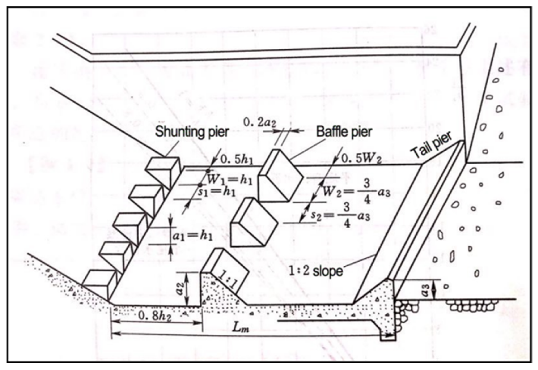
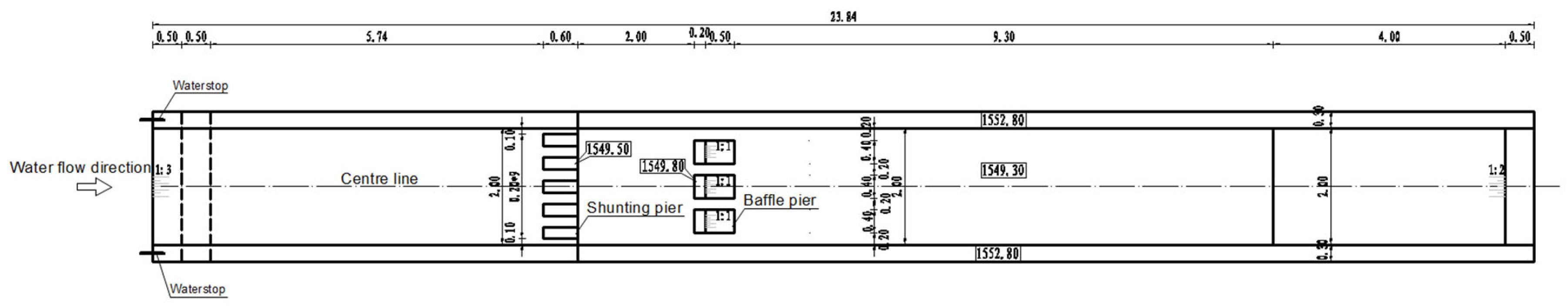
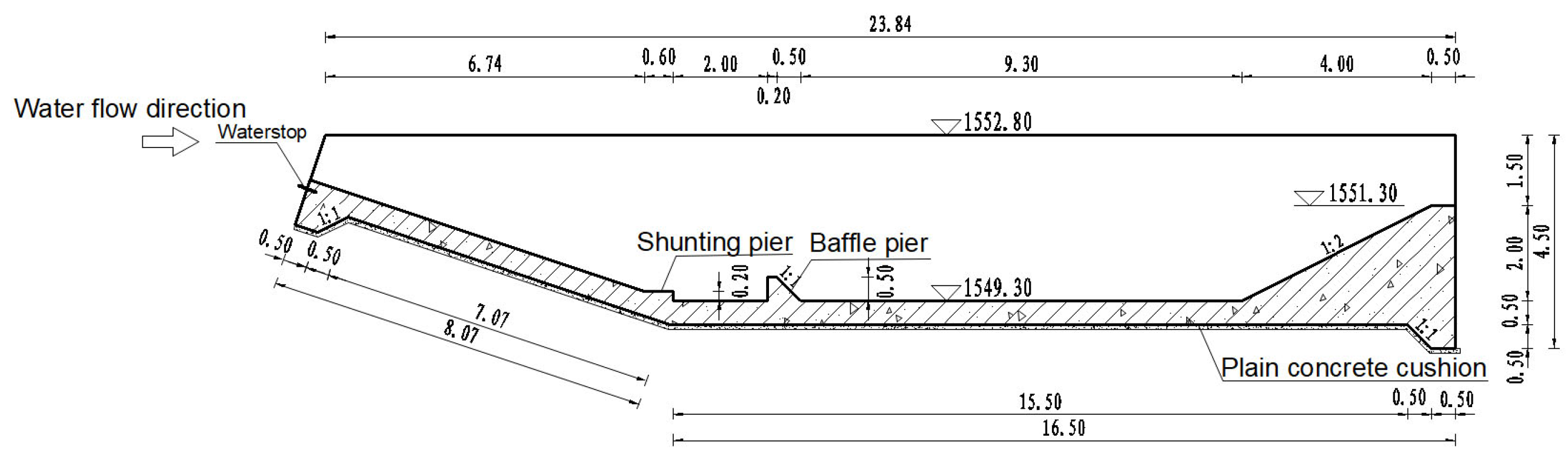
2.1. Structure of the Stilling Basin

The water discharge gate of the Jinchang Industrial Base Flood Storage Ecological Treatment Project uses a culvert gate. Due to the small rate of flow and large drop, it is suitable for a USBR III stilling basin (see Figure 1). However, the design parameters of the USBR III stilling basin are often determined through empirical formulas, which cannot be verified for their applicability and rationality through reasonable technical analysis methods. Conventional physical model tests are time-consuming and uneconomical, while having significant drawbacks for small and medium-sized projects. Therefore, it is necessary to seek better technical means and methods to verify and optimize the design of USBR III stilling basins.

2.2. Basic Principles of Numerical Simulation

The flow of water is governed by the law of physical conservation, which includes the laws of mass conservation, momentum conservation, and energy conservation. The main governing equations for this calculation are the conservation of mass equation and the momentum equation. As the flow is in a turbulent state, the calculation model also needs to follow additional turbulent transport equations.
(1)
Equation of Mass Conservation
Conservation of mass means that the mass of a substance will not change during movement. In a continuous medium, the mass conservation equation is an integral or differential continuity equation. The conservation of mass equation can be expressed as: the increase in mass in a fluid element per unit of time is equal to the net mass flowing into the element at the same time interval [17,18]. The equation is as follows:
𝜕 ρ 𝜕 t + 𝜕 ( ρ u ) 𝜕 x + 𝜕 ( ρ ν ) 𝜕 y + 𝜕 ( ρ ω ) 𝜕 z = 0
(2)
Momentum Conservation Equation
Conservation of energy refers to the energy conversion relationship between any two cross-sections of the same element flow or between different points on the same streamline in a constant total flow, and the total energy remains unchanged. The rate of change of momentum flowing in a micro element over time is equal to the sum of various forces acting on the micro element from the outside [19], and its equation is as follows:
𝜕 ρ u 𝜕 t + d i v ρ u u = d i v u g r a d u 𝜕 p 𝜕 x + 𝜕 ρ u ` 2 ¯ 𝜕 x 𝜕 ρ u ` v ` ¯ 𝜕 y 𝜕 ρ u ` v ` ¯ 𝜕 z + S u 𝜕 ρ v 𝜕 t + d i v ρ v u = d i v u g r a d v 𝜕 p 𝜕 x + 𝜕 ρ u ` v ` ¯ 𝜕 x 𝜕 ρ v ` 2 ¯ 𝜕 y 𝜕 ρ v ` w ` ¯ 𝜕 z + S v 𝜕 ρ w 𝜕 t + d i v ρ w u = d i v u g r a d w 𝜕 p 𝜕 x + 𝜕 ρ u ` w ` ¯ 𝜕 x 𝜕 ρ v ` w ` ¯ 𝜕 y 𝜕 ρ w ` 2 ¯ 𝜕 z + S w
The basic principle of numerical calculation is to replace the fields of physical quantities that were originally continuous in the time and spatial domains, such as velocity and pressure fields, with a set of variable values at a finite number of discrete points. Through certain principles and methods, an algebraic equation system is established regarding the relationship between the field variables at these discrete points, and then the algebraic equation system is solved to obtain approximate values of the field variables. The discrete method used in this calculation is the finite volume method.
In the discrete process, the key step is to calculate the parameter variables and their derivatives on the control volume through the node D-value, with the aim of establishing a discrete equation. The method of the D-value is often referred to as the discrete format. In this calculation, the more suitable second-order upwind scheme and QUICK scheme are used, which can significantly reduce numerical diffusion errors [20].
The discharge flow of water release structures is usually turbulent with high Reynolds numbers, and the flow is usually mixed with gas to form a multiphase flow [21,22]. The most widely used two-equation model for numerical simulation of high turbulent flow is the realizable k~ε model, which introduces equations about turbulent kinetic energy k and turbulent dissipation rate ε.
The mixture model is used for this calculation, with QUICK format for the volume fraction equation and second-order upwind format for the momentum equation and k~ε equation [23,24]. The PISO algorithm is used to calculate the pressure velocity coupling. The mixture model is commonly used to simulate the multiphase flow with different velocities between phases. It is a relatively simple multiphase flow model that assumes the relative balance of flow parameters between phases over short spatial distances and has strong coupling. The PISO algorithm can better satisfy the momentum equation and continuity equation, thereby accelerating the convergence rate in a single iterative step [25].

2.3. The Significance of Numerical Simulation Technology

The three main means to study fluid mechanics are numerical simulation, theoretical research, and model tests. Usually, these three research methods must cooperate with each other, complement each other, and promote each other, so as to jointly promote the development of fluid mechanics and solve various practical engineering problems.
The theoretical analysis method refers to putting forward various simplified flow models and establishing various mathematical control equations on the basis of studying the laws of fluid motion. Under certain assumptions and corresponding conditions, the analytical solution to the problem is obtained through a series of analytical derivations and operations. Many methods of theoretical analysis are often used in the preliminary design stage, but theoretical analysis cannot be used for complex and nonlinear flow phenomena.
The model test method is the main means to study the flow mechanism, analyze the flow phenomenon, explore and obtain the new concept of flow, and promote the development of fluid mechanics. Its disadvantage is that a series of complex technical problems need to be solved to complete a complete experimental process, which requires a long period and high research costs.
The characteristic of the numerical simulation method is that the internal details of the flow field can be obtained at less cost than that of the model test, and as long as the mathematical formulation of numerical simulation is correct, the quantitative results of the flow field can be given quickly within a wide range of flow parameters and physical design parameters, regardless of the inherent constraints of the test. Therefore, with the rapid development of computer fluid mechanics and computer science, numerical simulation has great potential in scientific and technological research. Mainly reflected in the following three aspects:
First, in a sense, the numerical simulation will have a deeper and more detailed understanding of the process of fluid movement than theoretical analysis and experimental research, so that not only the results of water flow movement can be obtained, but also the overall and local detailed behavior can be understood. Second, in the process of solving practical engineering problems, the optimal design scheme or test scheme can be selected by using simultaneous mathematical model simulation, so that the number of experiments, the period of experimental research and the corresponding expenses can be reduced. Third, numerical simulation can theoretically explore new phenomena and laws of fluid movement, and can replace some expensive and dangerous experiments that are difficult to realize through physical models in practical engineering, so it can be concluded that numerical simulation plays a vital role in fluid mechanics research and even the whole scientific and technological progress.

3. Model Construction and Parameter Determination

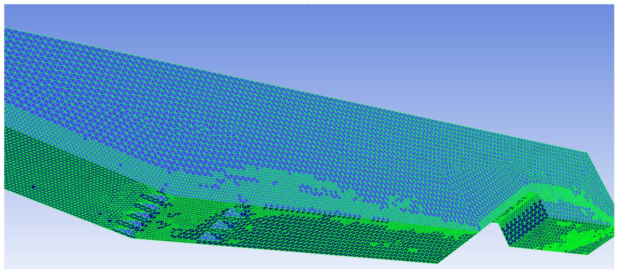
3.1. Model Construction

This study establishes a model and divides the grid based on the structure of the sluice and stilling basin of the flood storage ecological governance project in the Jinchang Industrial Base. There are two types of grids, namely the structured grid and unstructured grid [26]. The advantage of unstructured grids is that they can handle complex boundary shapes well, especially when dealing with irregular flow boundaries for simulating and calculating flow fields. The disadvantage is that they require a large amount of computation and require longer computation time. The geometric boundaries of the building in this case are complex, so a non-structural hexagonal mesh is used to discretize the calculation area, and the water flow area is locally densified during the calculation process. The number of grid cells in the model is 1,090,179, 1 cell zone, and 5 face zones.
The structural diagram of the sluice and grid division is shown in Figure 2, Figure 3 and Figure 4.

3.2. Boundary Parameters

(1)
Inlet boundary
Due to the two-phase flow of aerated water, the water inlet and air inlet are respectively set at the inlet boundary. The water inlet adopts velocity inlet boundary conditions. Given the initial average flow velocity Uin of the water flow at the inlet (Uin is given a flow velocity of 1.25 m3/s based on actual operating conditions), the turbulence kinetic energy kin at the inlet, and the turbulence energy dissipation rate distribution εin [27], their values are determined by the following equation:
k i n = 0.0144 U i n 2
ε i n = k i n 1.5 / 0.25 D
In the above equation, D = 2R, where R is the hydraulic radius of the cross-section of water.
The air inlet adopts a pressure inlet boundary, and the total pressure at the inlet boundary is given as atmospheric pressure. The pressure boundary is applicable when the inlet pressure is known.
(2)
Pressure boundary
The pressure boundary also adopts the pressure inlet boundary, with the pressure set at atmospheric pressure, which is more suitable for simulating water bodies with free surfaces [28].
(3)
Outlet boundary
At the outlet, the water flow and air are fully mixed and the water depth is difficult to determine. It can be set as the same outlet, and the outlet water flow is a free outflow. Therefore, setting the outlet as a pressure outlet allows the water flow and air to be freely adjusted at the outlet [29,30]. At the outlet boundary, assuming the flow is fully developed turbulence and the radial velocity v is equal to 0, the mathematical expression is:
𝜕 u 𝜕 x = 𝜕 k 𝜕 x = 𝜕 ε 𝜕 x = 0 , v = 0
(4)
Wall boundary
In practical engineering, due to the viscosity of water flow, especially in the viscous bottom layer near the wall, the water flow is approximately laminar, with a low Reynolds number and insufficient turbulence development. However, the turbulence model is only applicable to fully developed turbulence, so special treatment is needed for the numerical model in the wall area to make the water flow conform to the actual flow conditions. The commonly used method at present is the wall function method, which establishes a certain functional relationship between various physical parameters at the edge wall and various physical parameters of high turbulence in the fluid. After obtaining the parameters of the main flow area, the numerical values of various physical quantities in the near wall area can be obtained [31,32]. The relationship between shear stress on the wall τ and flow velocity U ¯ is:
τ = λ w U ¯
λ w = μ   / y           y +   <   11.6 ρ C μ     1 / 4 k 1 / 2 κ / I n ( E y + )   y + 11.6  
y + = ρ C μ     1 / 4 k 1 / 2 y / μ ; κ = 0.41 ; E = 9.8 ; C μ = 0.0845
In the equation, k is turbulent kinetic energy and y is the distance from the near wall node to the edge wall. The range of contact between the flow field and the building in this calculation is based on wall boundaries.

4. Simulation Calculation Results and Analysis

This simulation study strictly follows the actual operating conditions of the Jinchang project’s sluice scale, with an overcurrent flow of 5 m3/s and an open gate discharge. By using ANSYS Mechanical Enterprise Fluent 2020, the energy dissipation effect of the stilling basin is comprehensively judged from the aspects of aeration concentration, water flow velocity, turbulent dissipation rate, Reynolds number of water flow and total pressure of water flow in the stilling basin of the USBR III stilling basin.
(1)
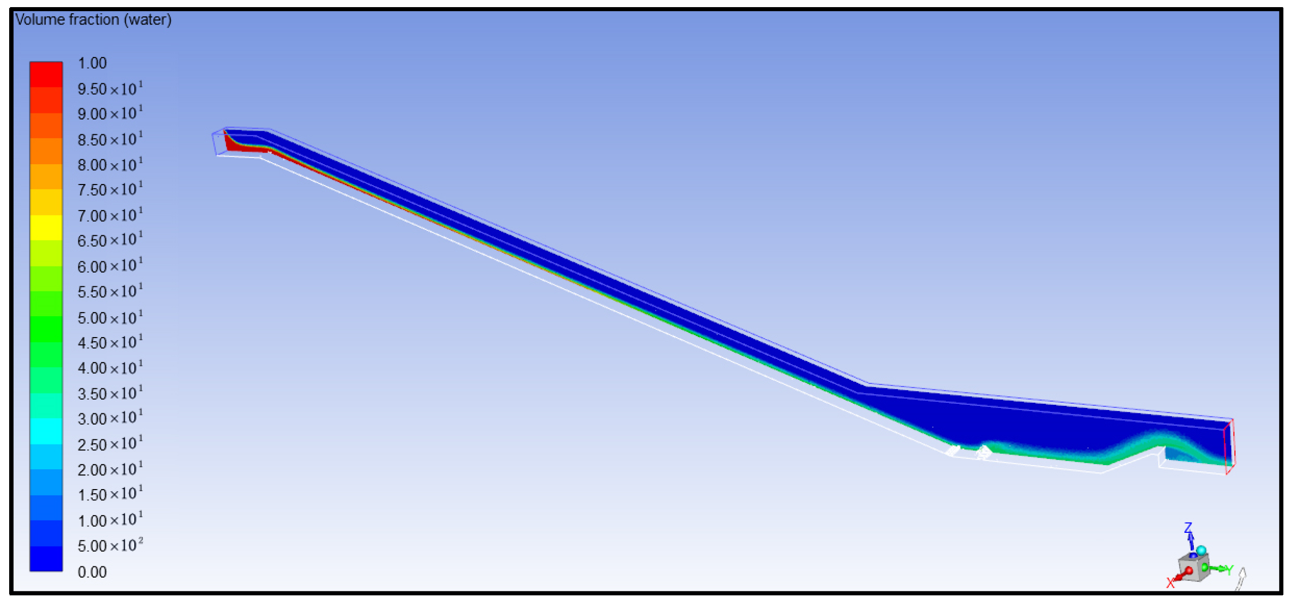
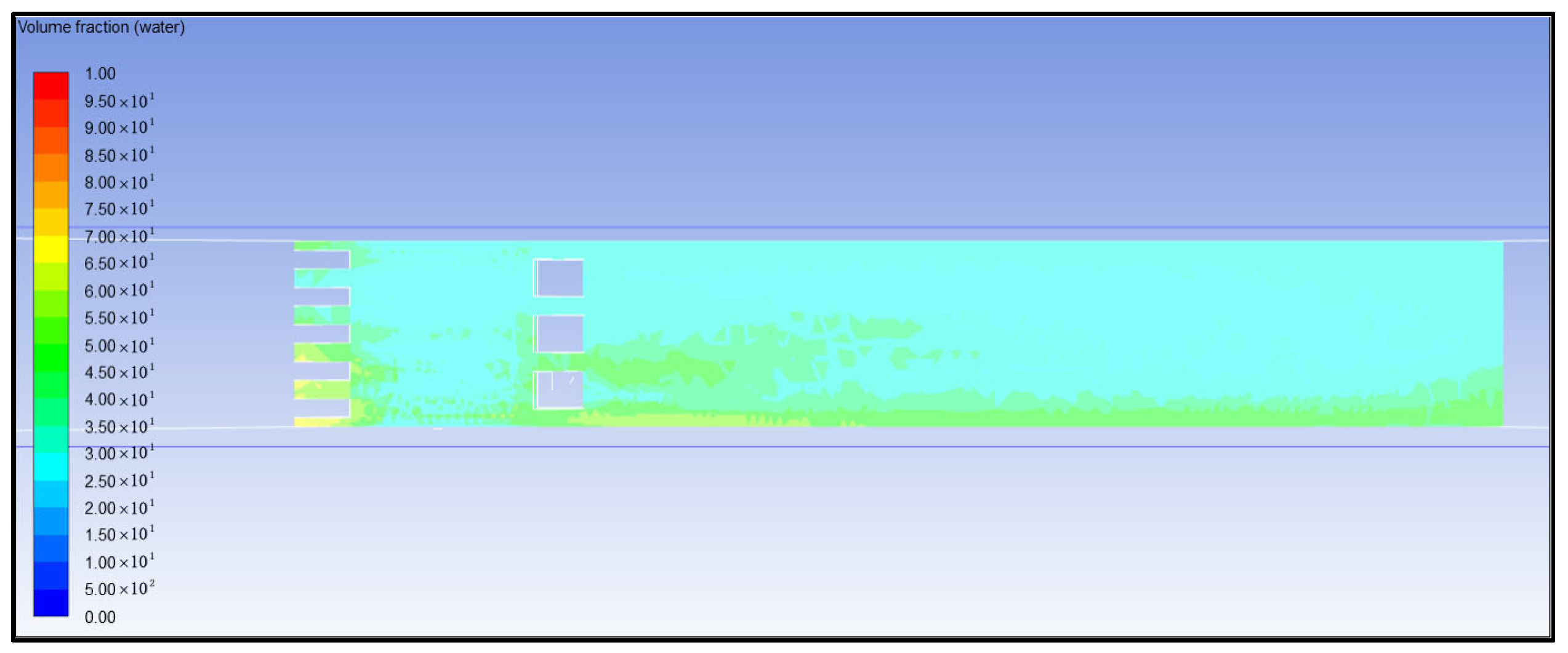
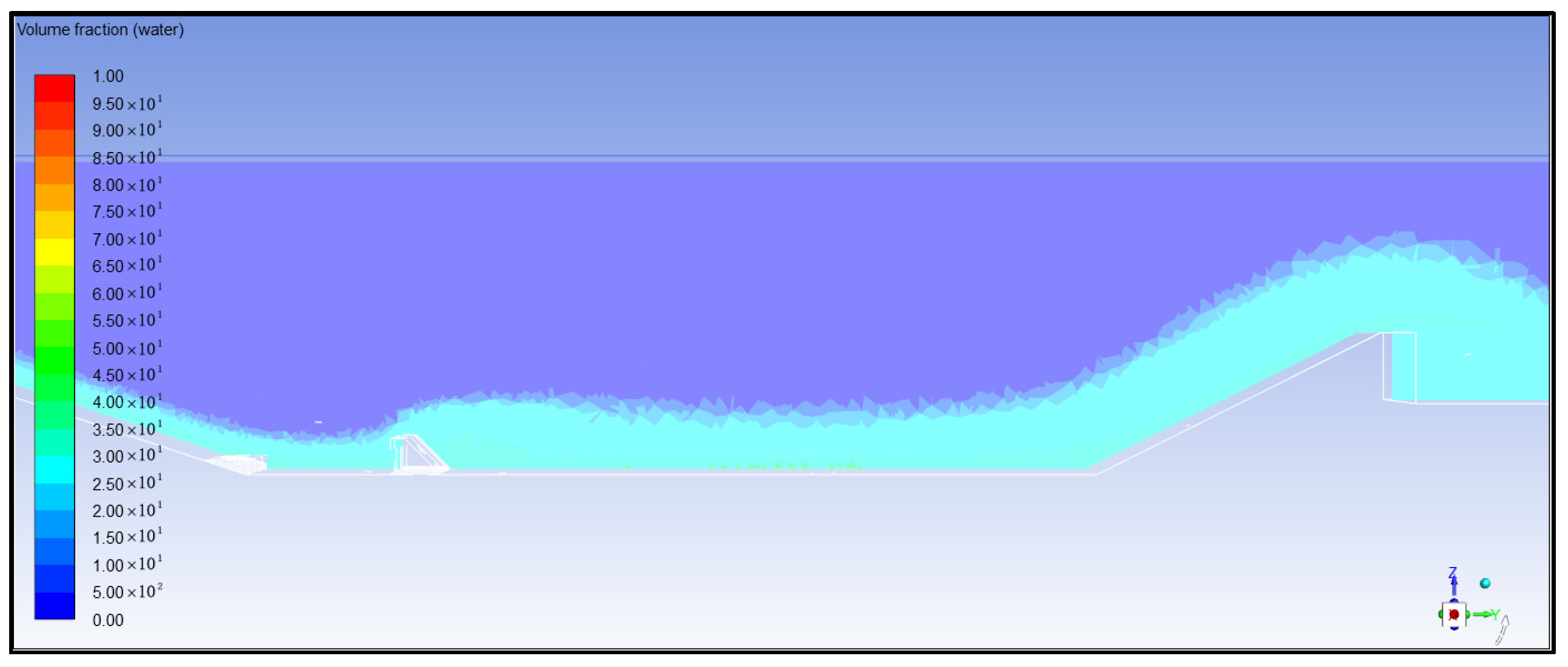
Analysis of Air Concentration
The simulation results of the aeration concentration in the USBR III stilling basin of the Jinchang project sluice are shown in Figure 5, Figure 6 and Figure 7.
According to the simulation calculation results of the aeration concentration in the USBR III stilling basin [33], it can be concluded that during the flow of water on steep slopes, the gas volume fraction ratio in the water gradually increases while the water volume fraction ratio gradually decreases, indicating that the aeration concentration in the water gradually increases (as shown in Figure 5). After passing through the stilling basin, the volume fraction of water reaches its lowest value, indicating that the water is turbulent and mixed with air in the pool. The water is fully aerated, and the energy dissipator effect is significant. The aeration concentration has reached the maximum value calculated in this study (as shown in Figure 7). From the analysis of the characteristic plane, sidewall turbulence is more severe than that in the middle part, which meets the design expectations (as shown in Figure 6).
(2)
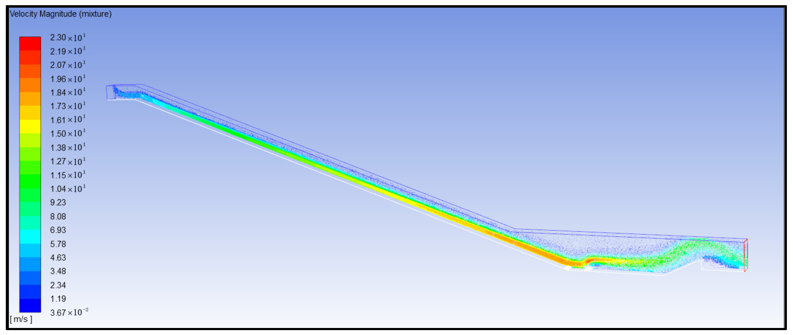
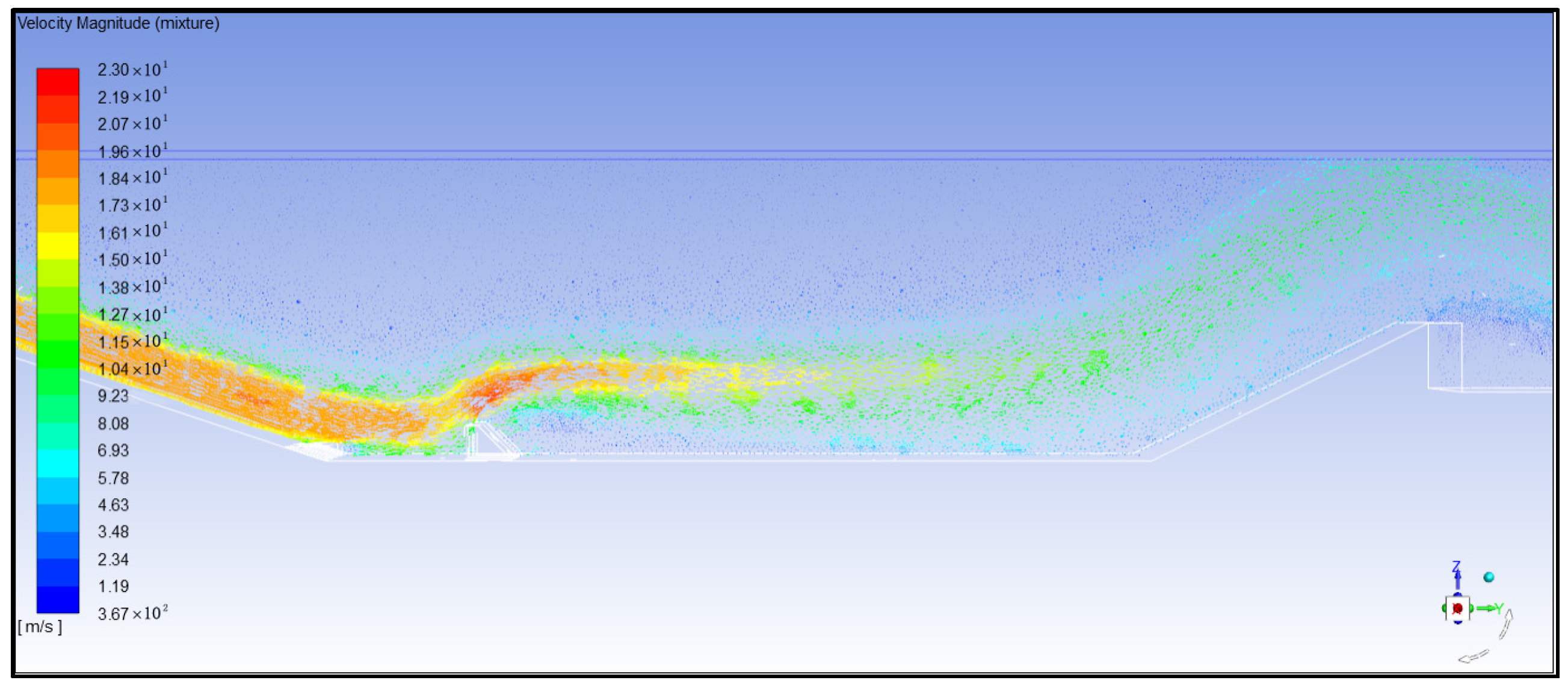
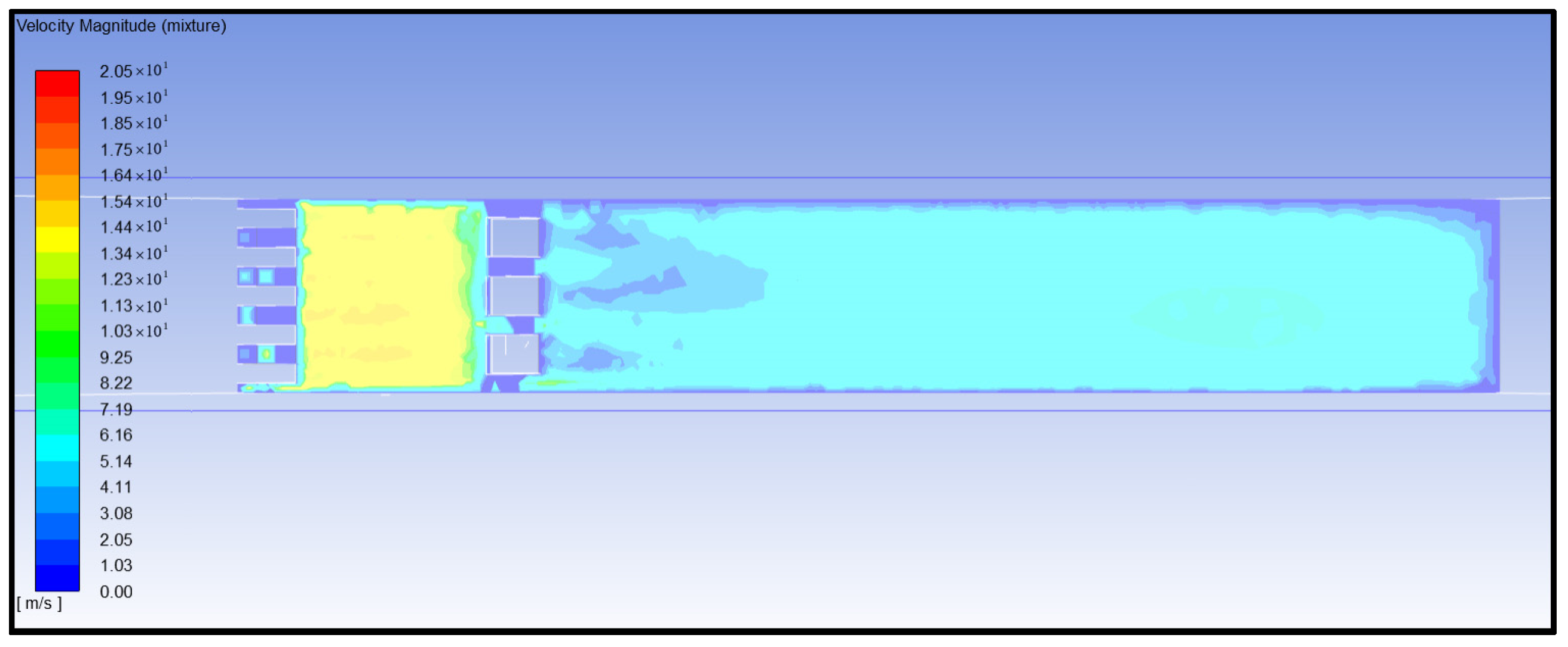
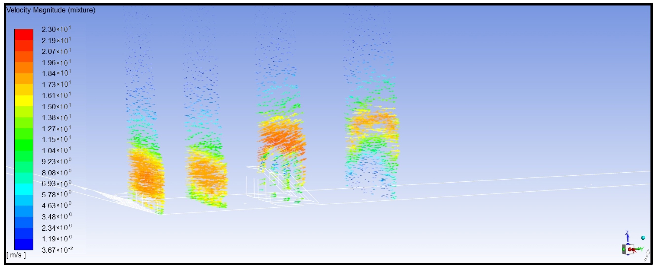
Analysis of water flow velocity
The analog computation results of water flow velocity in the USBR III stilling basin are shown in Figure 8, Figure 9, Figure 10, Figure 11, Figure 12 and Figure 13.
According to the simulation calculation results of the flow velocity of the USBR III stilling basin, it can be concluded that when the water flows through the slope section of the stilling basin, the potential energy of the water is converted into kinetic energy, and the flow velocity reaches a large value at the end of the slope section (as shown in Figure 8 and Figure 9). Then, the water flows through the diversion pier, impacts the baffle pier, and the local flow velocity reaches an extreme value. Subsequently, the water diffuses, splashes, and mixes with disturbances, resulting in a sharp decrease in kinetic energy and energy dissipation (as shown in Figure 10 and Figure 11), and the flow velocity decreases. When the water flows through the tailgate, the flow velocity decreases significantly. From the perspective of the cross-sectional analysis of water flow velocity, the flow velocity is relatively high within a certain vertical range of the energy dissipation system. As the water flow direction advances, the flow velocity tends to decrease within the vertical range (as shown in Figure 12 and Figure 13).
(3)
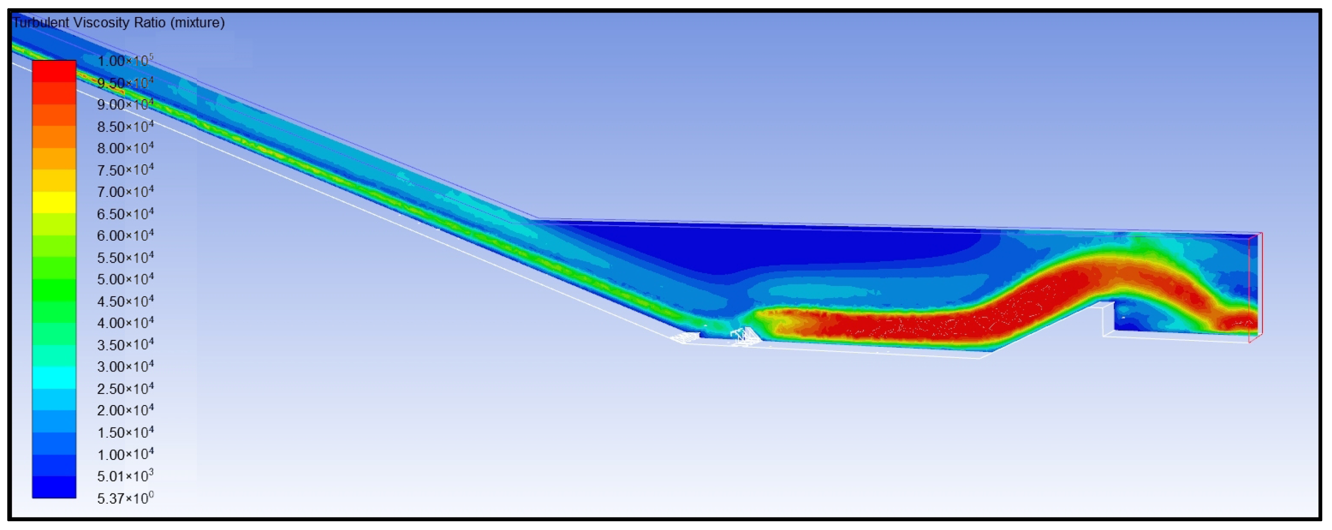
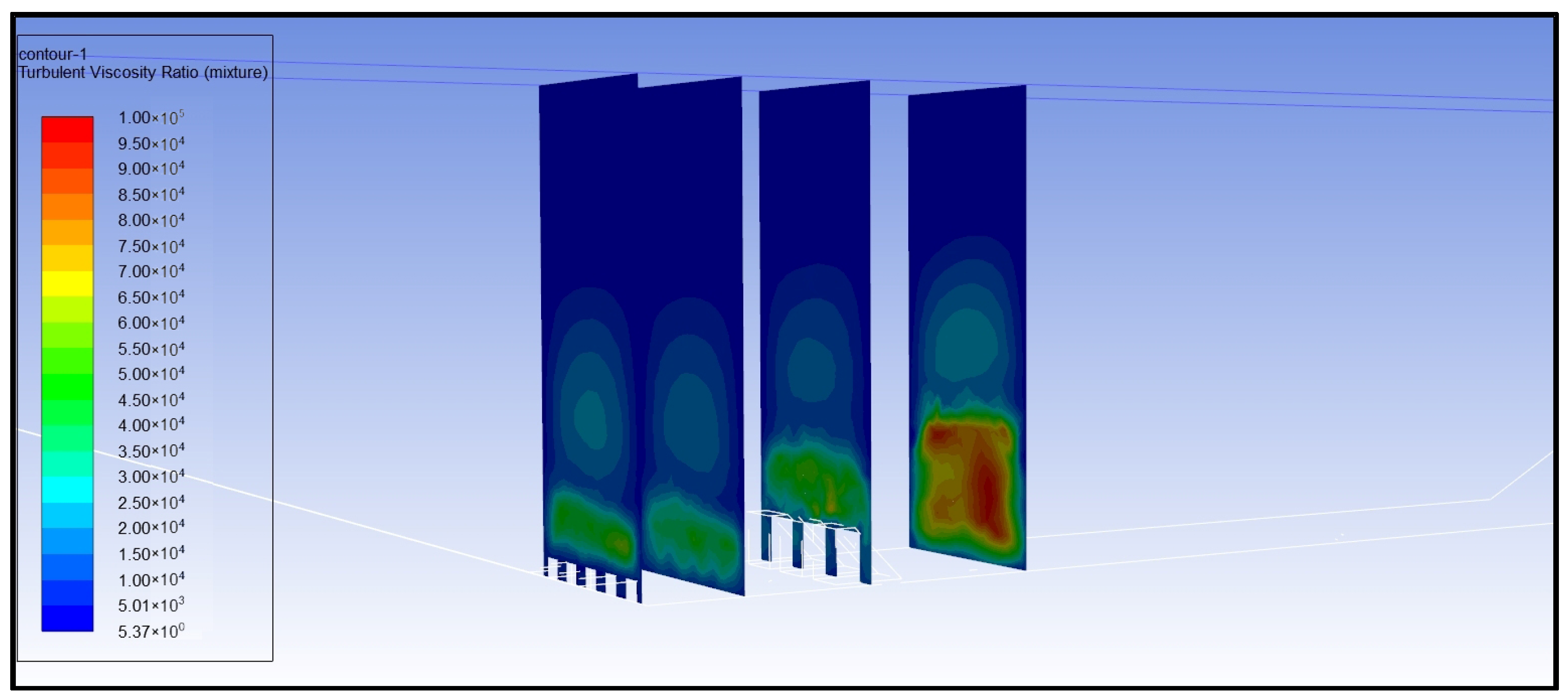
Analysis of Turbulent Dissipation Rate
The simulation results of the turbulent dissipation rate of the USBR III stilling basin are shown in Figure 14, Figure 15 and Figure 16.
According to the simulation calculation results of the turbulent dissipation rate of the USBR III stilling basin [34], it can be concluded that the severe occurrence area of turbulent dissipation rate is mainly concentrated on the downstream side of the baffle block in the downstream direction, and the trend gradually weakens (as shown in Figure 14 and Figure 15). From the perspective of characteristic plane analysis, the turbulent dissipation rate on the downstream side of the baffle block in the entire stilling basin is basically uniform and consistent (as shown in Figure 16).
(4)
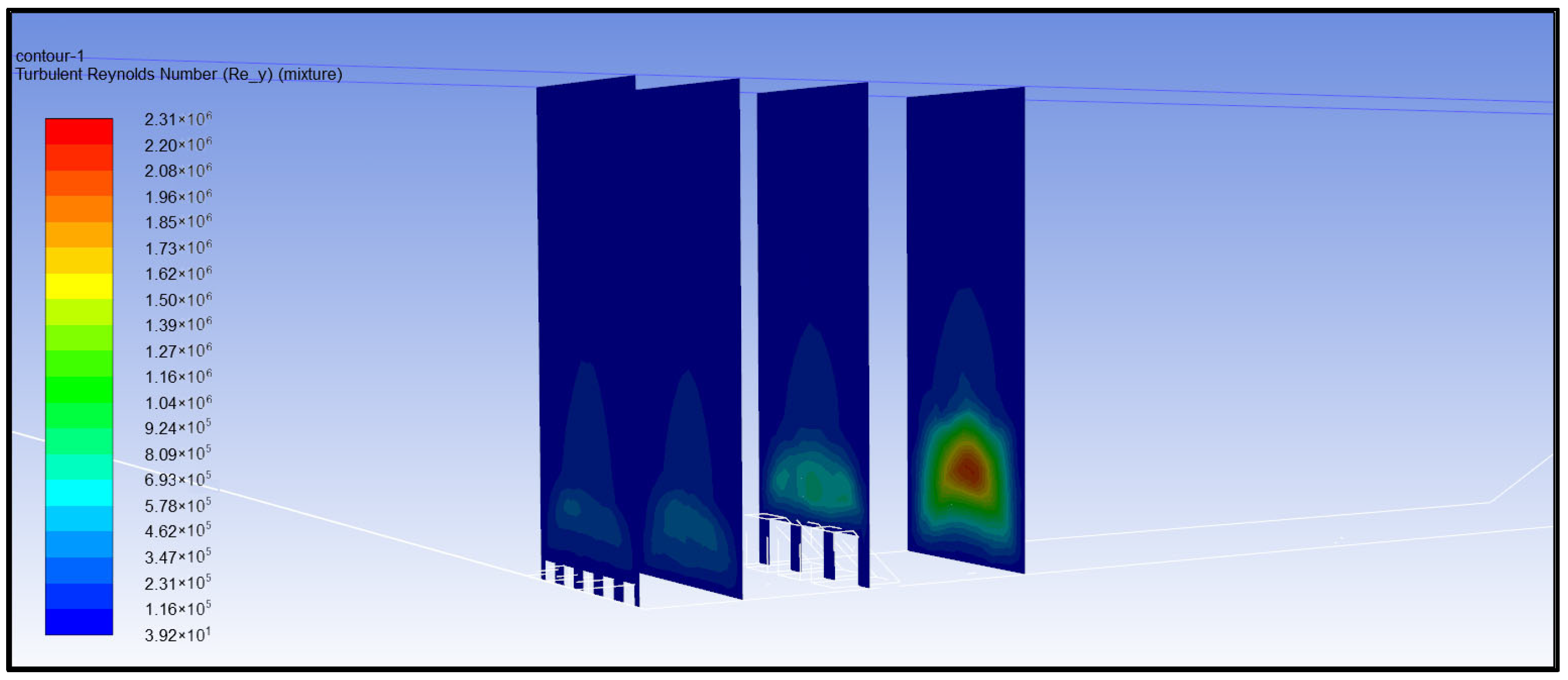
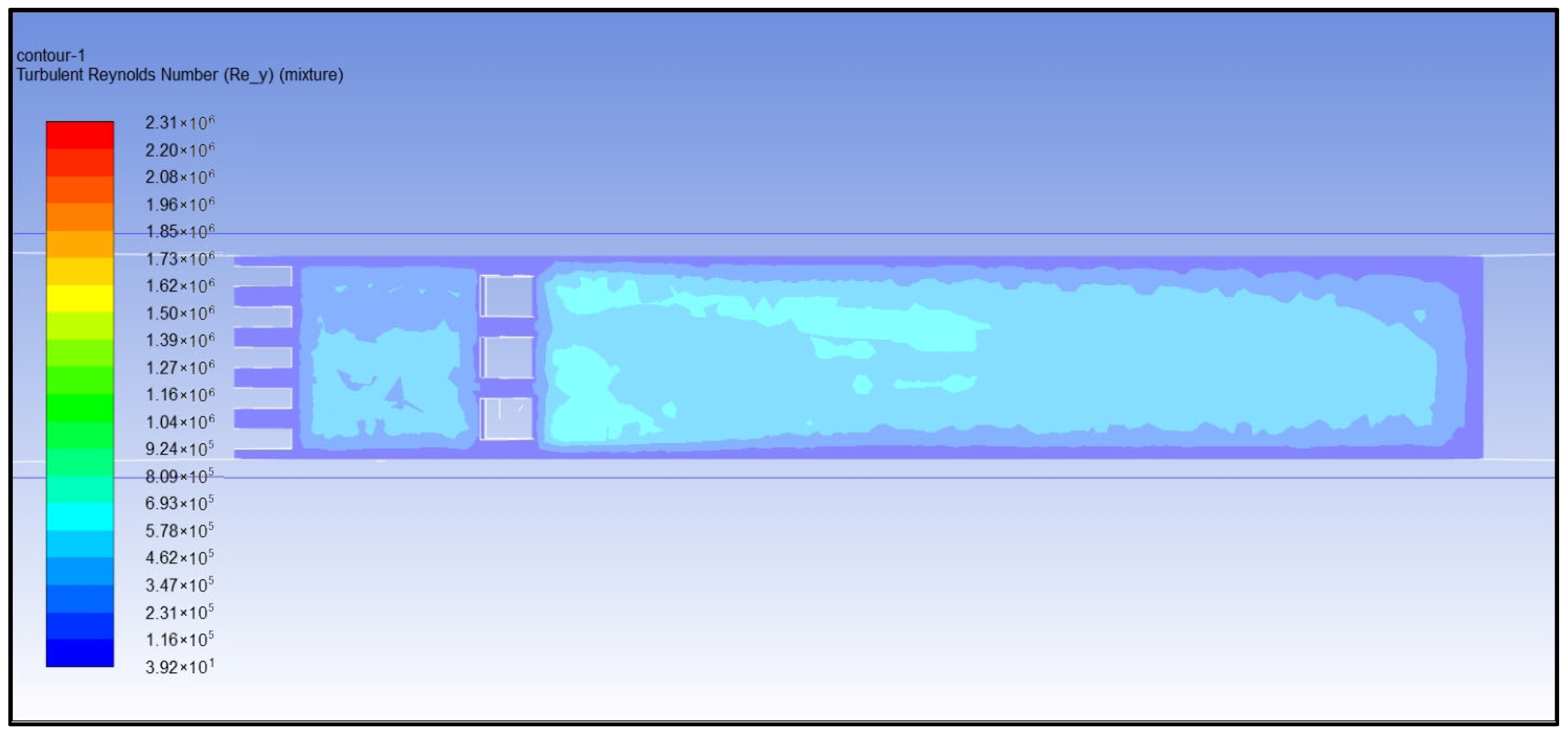
Reynolds number analysis of turbulent water flow
Under the simulated working conditions, the terminal velocity is 13.08 m/s, the slope length is 8.07 m, and the horizontal length is 16.50 m. The simulation results of the flow turbulent Reynolds number of the USBR III stilling basin are shown in Figure 17, Figure 18 and Figure 19.
According to the analog computation results of the turbulent Reynolds number of the USBR III stilling basin [35], it can be concluded that the main parameter indicators of the Reynolds number are flow velocity and water depth. The variation trend of the turbulent Reynolds number tends to be similar to the comprehensive trend of flow velocity and turbulent dissipation rate, that is, significant changes occur after the baffle block, and the length and magnitude of the change can be quantified (Figure 17, Figure 18 and Figure 19).
(5)
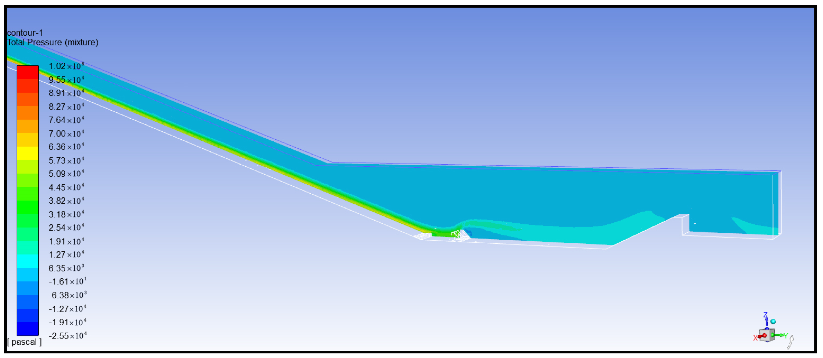
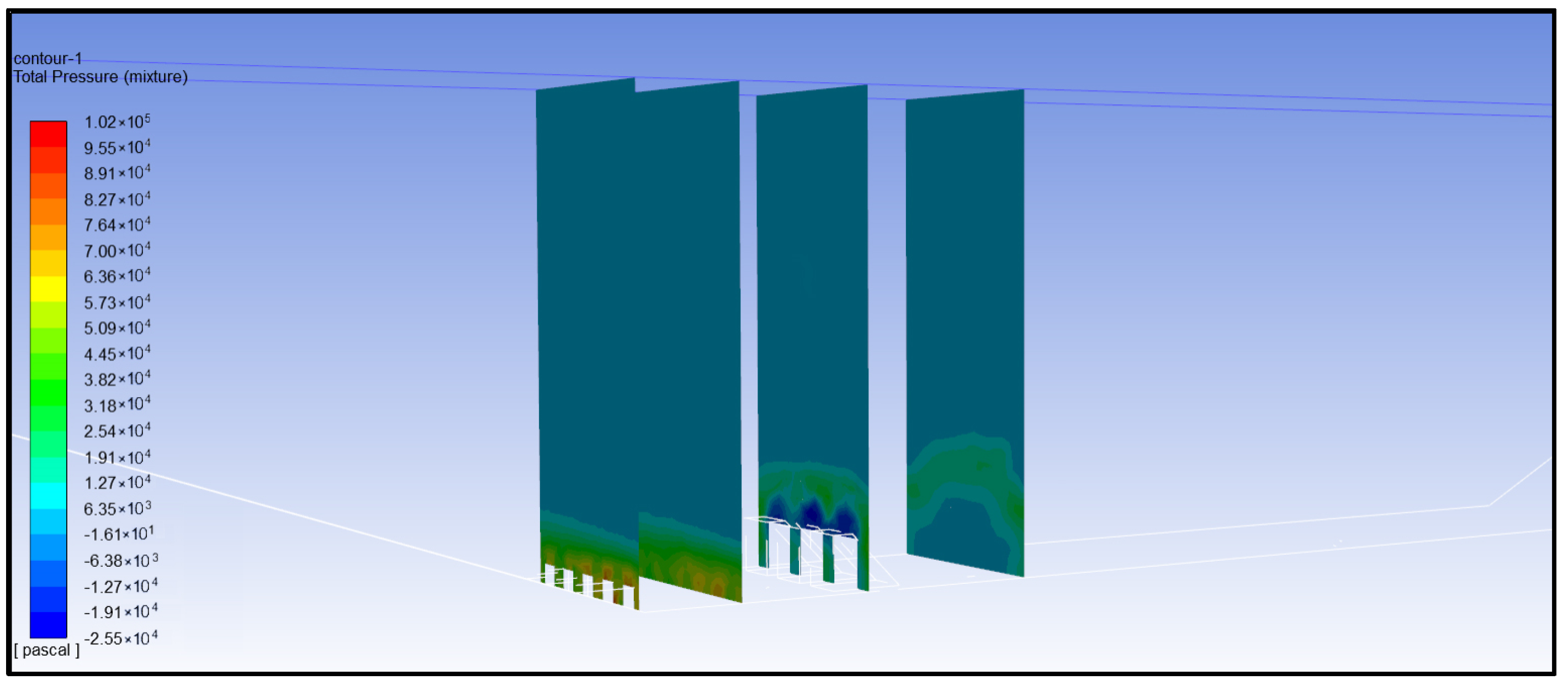
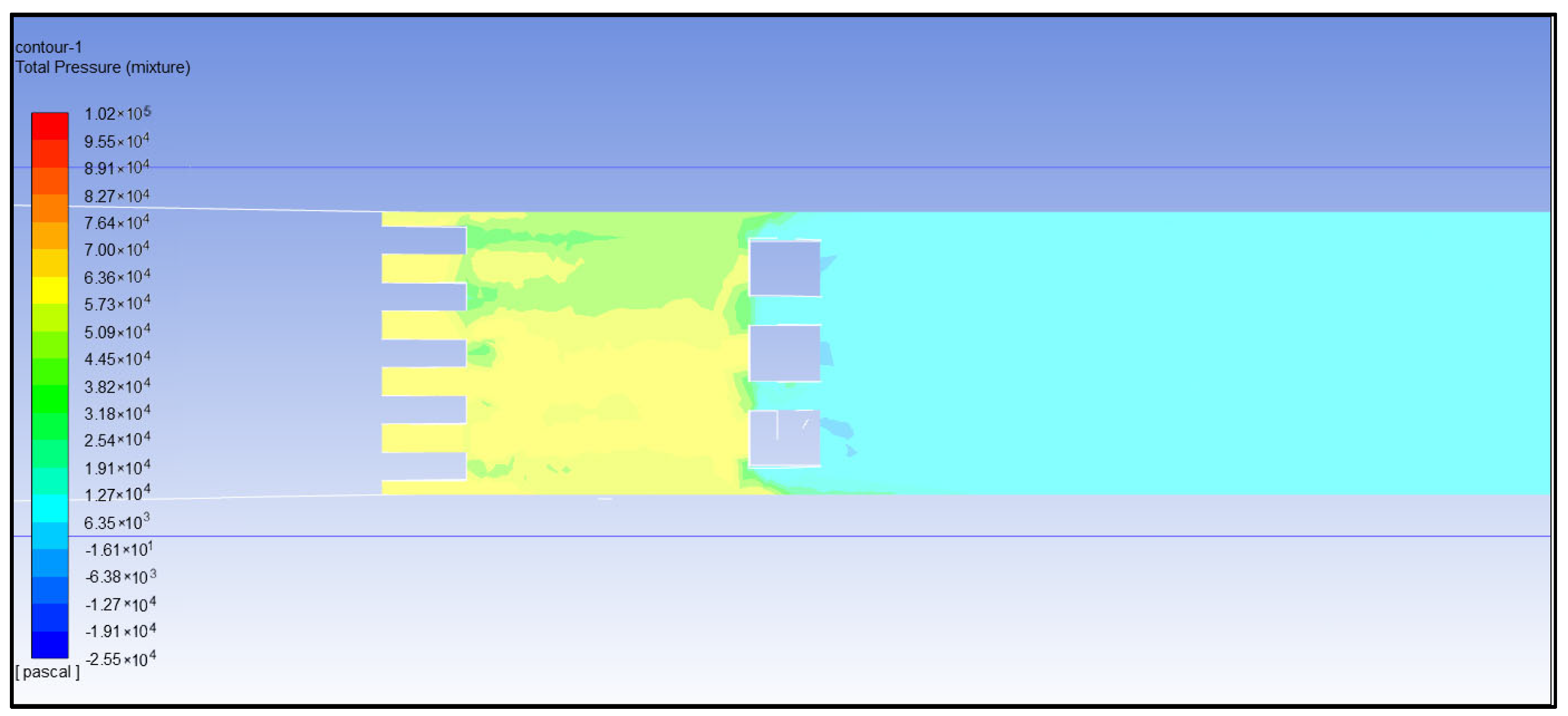
Analysis of total pressure of water flow
The analog computation results of the total pressure of the USBR III stilling basin water flow are shown in Figure 20, Figure 21 and Figure 22.
According to the simulation calculation results of the total pressure of water flow in the USBR III stilling basin [36], it can be concluded that the trend of the total pressure of the water flow mainly converges with the trend of the flow velocity. The numerical value is relatively large in the area between the diversion pier and the stilling pier. From the vertical simulation analysis, there is a significant weakening change in the total pressure at the location of the stilling pier (Figure 17, Figure 18 and Figure 19).
(6)
Comprehensive analysis
This simulation starts with the characteristic indicators related to flow velocity, water depth, volume, etc., and compares and analyzes the trend changes of energy dissipation from multiple perspectives such as plane, characteristic section, and facade. It basically covers the variation laws of the USBR III stilling basin in the process of energy dissipation, clarifies the specific parts of energy dissipation effect implementation, and demonstrates abstract energy dissipation problems more reasonably and intuitively. Through further quantitative analysis, technical support has also been provided for the optimization of the USBR III stilling basin in the Jinchang project.
Based on the high turbulence numerical simulation technique used in this study, and through repeated verification, the USBR III stilling basin was structurally optimized according to the changes in energy dissipation performance inside the original design of the Jinchang project. The optimized length of the stilling basin was shortened by nearly 2 m, accounting for 12% of the original calculated length (Table 1). Through the analysis of parameters such as the concentration of aeration, flow velocity, and turbulent dissipation rate in the characteristic section, the synergistic energy dissipation effect between the energy dissipator was verified, providing ideas for the reasonable combination of energy dissipator inside the USBR III stilling basin. The next step will be to conduct a more in-depth analysis, demonstrate the possibility of multiple combinations, improve the comprehensive energy dissipation efficiency of the USBR III stilling basin, and provide reference for its wide application.

5. Conclusions

The three-dimensional visualization high turbulence numerical simulation technique simulates the flow state and change process of water flow through numerical calculation. It can not only obtain various parameter results of water flow movement, but also is not affected by factors such as scale effect and instrument interference [37,38]. It has a strong applicability providing sufficient fine and accurate data and scientific support for the selection and design of hydraulic engineering shape schemes.
In the design of the sluice stilling basin for the ecological governance project of the Industrial Base in Jinchang City, the High Turbulence Numerical Simulation Technique was applied for verification, scientifically demonstrating the rationality of the scale of the stilling basin and the layout of the energy dissipator structure. Based on the simulation results, the length of the stilling basin was optimized, saving a large amount of work. At the same time, it intuitively displays the evolution of the entire energy dissipation process, providing technical support for the smooth application of the project and the realization of various benefits, with good social, environmental, and economic benefits, and because of effectively reducing project investment, it receives high praise from experts and the client.
In this paper, the optimization of USBRIII iii stilling basin is studied using a numerical simulation combined with specific examples, aiming at analyzing the accessibility of energy dissipation effect more intuitively and seeking the possibility of further optimization. On the other hand, the main design basis and main influencing parameters of this kind of stilling basin are excavated, and constructive design suggestions are put forward. Finally, the universal general formula of main parameters of the USBRIII iii stilling basin is summarized, which can guide and apply to such small and medium-sized projects, simplify the design process, and greatly promote the development of digital three-dimensional design technology. This further liberates the productive forces, making designers focus more on improving design quality and creative design. At the same time, this technical method has strong universality for the complex energy dissipation model of reservoir dams in water conservancy projects.

Author Contributions

Methodology, X.M.; Formal analysis, C.Z.; Data curation, X.W. and H.W.; Writing—original draft, X.M.; Writing—review & editing, Y.H. and D.B.; Supervision, W.W.; Project administration, B.Z.; Funding acquisition, C.Z. All authors have read and agreed to the published version of the manuscript.

Funding

The National Key Research and Development Program of China (grant No. 2023YFC3208604). The eco-hydrological model and flood and drought disaster risk assessment in the middle reaches of the Yellow River under a changing environment (grant No. U2243226). The innovation fund of the Yellow River Water Conservancy and Hydropower Development Group Co., Ltd. (grant No. DBAQJCZX2024001, DBAQJCZX2024002). The Xiaolangdi Dam safety monitoring platform project (grant No. XLDYX20026).

Data Availability Statement

Data is contained within the article.

Conflicts of Interest

Authors Xiao Meng, Chao Zhang and Bin Zhang were employed by the company Yellow River Engineering Consulting Co., Ltd. Author Wei Wang was employed by the company Yellow River Water Conservancy and Hydropower Development Group Co., Ltd. The remaining authors declare that the research was conducted in the absence of any commercial or financial relationships that could be construed as a potential conflict of interest.

References

  1. Yurdagul, S.K.; Kamil, I. Experimental and Numerical Modeling of Various Energy Dissipater Designs in Chute Channels. Appl. Water Sci. 2022, 12, 2–15. [Google Scholar]
  2. Viti, N.; Valero, D.; Gualtieri, C. Numerical Simulation of Hydraulic Jumps. Part 2: Recent Results and Future Outlook. Water 2018, 11, 28. [Google Scholar] [CrossRef]
  3. Valero, D.; Felder, S.; Kramer, M.; Wang, H.; Carrillo, M.J.; Pfister, M.; Bung, B.D. Air-water Flows. J. Hydraul. Res. 2024, 62, 319–339. [Google Scholar] [CrossRef]
  4. Zaffar, M.W.; Haasan, I.; Ghumman, A.R. Performance Evaluation of Different Stilling Basins Downstream of Barrage Using FLOW-3D Scour Models. Hydrology 2023, 10, 223. [Google Scholar] [CrossRef]
  5. Idfi, G.; Lasminto, U.; Kartika, A.A. Modification of USBR Type III Stilling Basin Using a Stepp Stair Model to Improve Hydraulic Performance and Energy Dissipation Effectiveness. J. Propuls. Technol. 2024, 45, 5403–5407. [Google Scholar]
  6. Badas, G.M.; Rossi, R.; Garau, M. May a Standard VOF Numerical Simulation Adequately Complete Spillway Laboratory Measurements in an Operational Context? The Case of Sa Stria Dam. Water 2020, 12, 1606. [Google Scholar] [CrossRef]
  7. Khadka, P.; Rai, S. Numerical Model Scenario Analysis of Stilling Basin: A Case Study of Tanahu Hydropower Project (140 MW). Int. J. Eng. Technol. 2023, 1, 153–165. [Google Scholar] [CrossRef]
  8. Zaffar, M.W.; Hassan, I.; Latif, U.; Jahan, S.; Ullah, Z. Numerical Investigation of Scour Downstream of Diversion Barrage for Different Stilling Basins at Flood Discharge. Sustainability 2023, 15, 11032. [Google Scholar] [CrossRef]
  9. Francisco, J.M.; José, F.V.; Rafael, G. Assessment of the Performance of a Modified USBR Type II Stilling Basin by a Validated CFD Model. J. Irrig. Drain. Eng. 2021, 147, 04021052. [Google Scholar]
  10. Su, X.Y.; Li, S.P.; Wang, M.M.; Cui, H.; Pan, K.; Yuan, J.; He, S. Numerical Simulation on Hydraulic Performance for Spillway Bends in Goushuipo Reservoir. Water Resour. Dev. Res. 2023, 23, 67–74. [Google Scholar]
  11. Liu, L.Y. Analysis of River Ecological Management Solution of Jinyuan District. Water Resour. Dev. Res. 2024, 24, 54–58. [Google Scholar]
  12. Wang, X.D. Analysis of the Impact of the Floating Bridge Project in Changtu County on the Flow Field of the Liaohe River. Water Resour. Dev. Res. 2016, 16, 55–57. [Google Scholar]
  13. Wei, L.W.; Hu, K.; Niu, G.L. Digital Twin Xiaolangdi: Construction and application of dam safety monitoring and management platformr. Water Resour. Dev. Res. 2024, 6, 2–8. [Google Scholar]
  14. Wang, C.; Jia, X.; Peng, Y.; Gao, Z.; Yu, H. Transient Sand Scour Dynamics Induced by Pulsed Submerged Water Jets: Simulation Analysis. J. Mar. Sci. Eng. 2024, 12, 2041. [Google Scholar] [CrossRef]
  15. Totu, A.-G.; Olariu, C.-T.; Trifu, A.-T.; Totu, A.-C.; Cican, G. Development and Assessment of a Miniaturized Test Rig for Evaluating Noise Reduction in Serrated Blades Under Turbulent Flow Conditions. Acoustics 2024, 6, 978–996. [Google Scholar] [CrossRef]
  16. Chen, D.; Liu, H.; Hua, L.; Ji, Z.; Lu, T. Drops and Steep Slopes; China Water & Power Press: Beijing, China, 2009; p. 167. [Google Scholar]
  17. Kambe, T. New Perspectives on Mass conservation Law and Waves in Fluid Mechanics. Fluid Dyn. Res. 2020, 52, 2–15. [Google Scholar] [CrossRef]
  18. Cercos-Pita, J.L.; Dalrymple, R.A.; Herault, A. Diffusive Terms for the Conservation of Mass Equation in SPH. Appl. Math. Model. 2016, 40, 8722–8736. [Google Scholar] [CrossRef]
  19. Heo, J.; Kim, K.D.; Kim, B.J. Improvement of One-Dimensional Two-Fluid Momentum Conservation Equations for Vertically Stratified Flow. Nucl. Technol. 2018, 204, 162–171. [Google Scholar] [CrossRef]
  20. Zhang, Y.; Zhang, L.P.; He, X.; Deng, X.G. An Improved Second-Order Finite-Volume Algorithm for Detached-Eddy Simulation Based on Hybrid Grids. Commun. Comput. Phys. 2016, 20, 459–485. [Google Scholar] [CrossRef]
  21. Shaheed, R.; Mohammadian, A.; Gildeh, H.K. A Comparison of Standard k–ε and Realizable k–ε Turbulence Models in Curved and Confluent Channels. Environ. Fluid Mech. 2019, 19, 543–568. [Google Scholar] [CrossRef]
  22. Fuhrman, D.R.; Li, Y.Z. Instability of the Realizable k–ε Turbulence Model Beneath Surface Waves. Phys. Fluids 2020, 32, 2–15. [Google Scholar] [CrossRef]
  23. Jaki, T.; Su, T.L.; Kim, M.; Van Horn, M.L. An Evaluation of the Bootstrap for Model Validation in Mixture Models. Commun. Stat.-Simul. Comput. 2018, 47, 1028–1038. [Google Scholar] [CrossRef] [PubMed]
  24. Lubke, G.H.; Luningham, J. Fitting Latent Variable Mixture Models. Behav. Res. Ther. 2017, 98, 91–102. [Google Scholar] [CrossRef] [PubMed]
  25. Venier, C.M.; Pairetti, C.I.; Damian, S.M.; Nigro, N.M. On the Stability Analysis of the PISO Algorithm on Collocated Grids. Comput. Fluids 2017, 147, 25–40. [Google Scholar] [CrossRef]
  26. Zhong, D.D.; Sheng, C.H. A New Method towards High-order Weno Schemes on Structured and Unstructured Grids. Comput. Fluids 2020, 200, 104453. [Google Scholar] [CrossRef]
  27. Lewandowski, M.T.; Pluszka, P.; Pozorski, J. Influence of Inlet Boundary Conditions in Computations of Turbulent Jet Flames. Int. J. Numer. Methods Heat Fluid Flow 2018, 28, 1433–1456. [Google Scholar] [CrossRef]
  28. Yildiran, I.N.; Beratlis, N.; Capuano, F.; Loke, Y.H.; Squires, K.; Balaras, E. Pressure Boundary Conditions for Immersed-boundary Methods. J. Comput. Phys. 2024, 510, 113057. [Google Scholar] [CrossRef]
  29. Hu, F.Y.; Wang, Z.D.; Tamai, T.; Koshizuka, S. Consistent Inlet and Outlet Boundary Conditions for Particle Methods. Int. J. Numer. Methods Fluids 2019, 92, 1–19. [Google Scholar] [CrossRef]
  30. Alvarado-Rodríguez, C.E.; Klapp, J.; Sigalotti, L.D.; Dominguez, J.M.; Sánchez, E.D.C. Non-reflecting Outlet Boundary Conditions for Incompressible Flows Using SPH. Comput. Fluids 2017, 159, 177–188. [Google Scholar] [CrossRef]
  31. Aleksin, V.A.; Utyuzhnikov, S.V. Implementation of Near-wall Boundary Conditions for Modeling Boundary Layers with Free-stream Turbulence. Appl. Math. Model. 2014, 38, 3591–3606. [Google Scholar] [CrossRef]
  32. Nguyen, T.M.; Aly, A.M.; Lee, S.W. Improved Wall Boundary Conditions in the Incompressible Smoothed Particle Hydrodynamics Method. Int. J. Numer. Methods Heat Fluid Flow 2018, 28, 704–725. [Google Scholar] [CrossRef]
  33. Bai, R.D.; Zhang, F.X.; Liu, S.J.; Wang, W. Air Concentration and Bubble Characteristics Downstream of a Chute Aerator. Int. J. Multiph. Flow 2016, 87, 156–166. [Google Scholar] [CrossRef]
  34. Wang, G.C.; Yang, F.; Wu, K.; Ma, Y.F.; Peng, C.; Liu, T.S.; Wang, L.P. Estimation of the Dissipation Rate of Turbulent Kinetic Energy: A Review. Chem. Eng. Sci. 2020, 29, 2–14. [Google Scholar] [CrossRef]
  35. Kumar, P.; Sharma, A. Reynolds Number Effect on the Parameters of Turbulent Flows over Open Channels. Aqua-Water Infrastruct. Ecosyst. Soc. 2024, 73, 1030–1047. [Google Scholar] [CrossRef]
  36. Monteiro, L.R.; Lucchese, L.V.; Schettini, E.B.C. Comparison between Hydrostatic and Total Pressure Simulations of Dam-break Flows. J. Hydraul. Res. 2019, 58, 725–737. [Google Scholar] [CrossRef]
  37. Wang, Y.H.; Bao, Z.J.; Wang, B. Three-dimensional Numerical Simulation of Flow in Stilling Basin Based on Flow-3D. Eng. J. Wuhan Univ. 2012, 45, 454–457. [Google Scholar]
  38. Xu, W.L.; Liao, H.S.; Yang, Y.Q.; Wu, C.G. Numerical Simulation of 3-D Turbulent Flows of Plunge Pool and Energy Dissipation Analysis. J. Hydrodyn. 1996, 11, 561–569. [Google Scholar]
Figure 1. Diagram of a typical USBR III Stilling Basin [16].
Water 16 03568 g001
Figure 2. Plan of USBR III stilling basin for the Jinchang project.
Water 16 03568 g002
Figure 3. Typical elevation of USBR III stilling basin in the Jinchang project.
Water 16 03568 g003
Figure 4. Sketch Map of grid division for USBR III stilling basin in the Jinchang project.
Water 16 03568 g004
Figure 5. Distribution nephogram of overall volume fraction of water flow in the calculation area.
Water 16 03568 g005
Figure 6. Distribution nephogram of volume fraction of water flow at a pool bottom elevation of +0.2 m.
Water 16 03568 g006
Figure 7. Distribution nephogram of water flow volume fraction.
Water 16 03568 g007
Figure 8. Distribution nephogram of overall velocity vector of water flow in the calculation area.
Water 16 03568 g008
Figure 9. Distribution nephogram of flow velocity vector.
Water 16 03568 g009
Figure 10. Distribution nephogram of flow velocity at a pool bottom elevation of +0.2 m.
Water 16 03568 g010
Figure 11. Vector diagram of water flow velocity at the bottom elevation of +0.2 m.
Water 16 03568 g011
Figure 12. Vector diagram of flow velocity distribution in characteristic section.
Water 16 03568 g012
Figure 13. Distribution nephogram of flow velocity distribution in characteristic section.
Water 16 03568 g013
Figure 14. Overall distribution nephogram of the turbulent dissipation rate of water flow in the calculation area.
Water 16 03568 g014
Figure 15. Typical section flow turbulence dissipation rate.
Water 16 03568 g015
Figure 16. Distribution nephogram of the turbulent dissipation rate at a pool bottom elevation of +0.2 m.
Water 16 03568 g016
Figure 17. Overall distribution nephogram of the turbulent Reynolds number of water flow in the calculation area.
Water 16 03568 g017
Figure 18. Distribution nephogram of the Reynolds number of turbulent flow in the characteristic section.
Water 16 03568 g018
Figure 19. Distribution nephogram of the turbulent Reynolds number at a bottom elevation of +0.2 m.
Water 16 03568 g019
Figure 20. Overall distribution nephogram of total pressure of water flow in the calculation area.
Water 16 03568 g020
Figure 21. Distribution nephogram of total pressure of characteristic section water flow.
Water 16 03568 g021
Figure 22. Distribution nephogram of total pressure at a pool bottom elevation of +0.2 m.
Water 16 03568 g022
Table 1. Comparison of typical parameters before and after optimization of tail sill section of stilling basin.
PejectLengthAir ConcentrationWater Flow Velocity
(m/s)
Turbulent Dissipation RateReynolds NumberTotal Pressure of Water Flow (kpa)
Before optimization16.50.2~0.42.25~3.92(4.6~8.8) × 104(5.2~8.6) × 10510.5~17.3
After optimization14.60.1~0.32.05~4.11(5.0~8.5) × 104(5.8~9.2) × 10512.7~19.1
Disclaimer/Publisher’s Note: The statements, opinions and data contained in all publications are solely those of the individual author(s) and contributor(s) and not of MDPI and/or the editor(s). MDPI and/or the editor(s) disclaim responsibility for any injury to people or property resulting from any ideas, methods, instructions or products referred to in the content.

