Exploring Similarities and Differences in Water Level Response to Earthquakes in Two Neighboring Wells Using Numerical Simulation

Abstract

The seismic effect of well water level is complex and variable, and even if both wells are located in an area with similar tectonic and hydrogeological conditions, they exhibit slightly varying response characteristics to the same earthquake. Wells BB and RC, located about 100 km apart in the southwest of the Huayingshan fault zone in the Sichuan and Chongqing regions, exhibited obvious similarities and differences in their co-seismically response and sustained recovery characteristics during the Wenchuan Ms8.0 earthquake. Based on the dislocation theory and fluid–solid coupling theory, this study developed the seismic stress–strain model and the response model of pore pressure to seismic stress using Coulomb 3.3 and COMSOL 6.3, respectively. Simulation findings indicate that both BB and RC are located in the expansion zone, where their water levels show a co-seismic step-down. The amplitudes of BB and RC water levels are 83 cm and 81 cm, which are approximately 10 cm smaller than the actual values. The recovery times are 60 d for BB and 3 h for RC, closely resembling the actual values. Furthermore, the numerical results from different scenarios show that the recovery time of pore pressure is reduced by several times when the permeability of the confining layer overlying the observed aquifer increases by one order of magnitude or the thickness decreases, and this change is more sensitive to the permeability. It is clear that the confining condition has an important impact in the response time of sustained changes in well water levels, which may also help to explain the variations in the characteristics of sustained changes in wells BB and RC.

1. Introduction

Seismic activity can cause a variety of hydrological responses, the most common of which is the changes in well water level [1]. The seismic stress induced by focal fault rupture will cause corresponding changes in volumetric strain, pore pressure, and even hydrogeological parameters in an aquifer [2,3], which eventually manifest as changes in well water level. As a result, a well-closed confined well can be used as a “sensitive manometer” to monitor the crustal stress activity [4,5,6]. The co-seismic changes in well water level are the most direct form of seismic stress acting on the well-aquifer system [7], which includes both static tectonic stress and dynamic seismic stress. In the near field, the groundwater level is primarily determined by tectonic stress induced by focal fault rupture, which is often depicted as step changes [8,9]. The groundwater level in the far field is mostly controlled by dynamic seismic stress [10], and the magnitude of the energy is proportional to the amplitude of the seismic wave and the epicenter distance [11,12,13]. Currently, the main far-field response mechanisms include the consolidation and compaction of loose sediments, rupture of hard rocks, periodic deformation of aquifers, permeability changes, and so on [11,14,15,16,17,18,19]. In the midfield, the groundwater level changes are affected by both static stress and dynamic stress [20,21]. In addition, the co-seismic response pattern of well water levels is influenced not only by seismic stress [22] but also by other factors such as wellbore structure [23], aquifer characteristic and tectonic condition [24,25,26]; so, it often behaves complexly and variously. Meanwhile, a large number of observational data indicate that there is also significant variability in the duration of the response of well water levels to earthquakes, which often ranges from a few minutes to several months [27]. Studying this continuous changing process will aid in understanding the response mechanism and influencing factors of earthquake-induced variations in well water level [28], and there may be some association between the well water level response and the confining condition of an aquifer [29,30]. However, most current studies on their relationship focus on the co-seismic response of well water level but ignore the ongoing evolution of well water levels after an earthquake. The study of this sustained change process can help to enhance the understanding of the influencing factors and response mechanism of seismic well water level, as well as serve a reference for further research into the interaction between aquifer system and seismic activities.

Due to the complexity of site hydrogeological conditions and the episodic nature of seismic hazards, numerical analysis techniques are gradually being applied to study topics related to various natural hazards. The simulation of groundwater response during earthquakes in Taiwan using the finite element software ABAQUS shows that hydrogeological characteristics have an important influence on earthquake-induced changes in groundwater levels [28]. Numerical analysis of well water data from the Canterbury Plain, New Zealand, reveals a decline in infiltration rates in the region after the 2010 earthquake [31]. Volcanic groundwater monitoring in the Canary Islands, Spain, provided valuable insights into volcanic activity, where chemical anomalies in groundwater composition were recognized as precursors of volcanic activity [32]. In addition, a porous media flow model (TOUGH2) was used to successfully simulate the recovery process of well water levels in the Italian region after the 2012 Emilia earthquake with good simulation results [23]. With the PDFLOW program, the researchers successfully simulated the perturbation of aquifer pore pressure during the chi-chi earthquake [33]. Numerical analysis methods can reveal the hydraulic interactions between the aquifer and the surrounding clay after experiencing seismic vibrations [34]. After the Ms8.0 Wenchuan earthquake in 2008, our research team has been tracking the response characteristics of the well water level to various strong earthquakes in the Sichuan, Yunnan, Shaanxi, Gansu and Chongqing regions. It is found that wells BB and RC in the Sichuan and Chongqing areas are both located in the Huayingshan fault zone, and the two wells have similar regional tectonic and hydrogeological conditions, with the observed layer lithology being feldspathic sandstone. However, the response of the well water level to multiple earthquakes showed the obvious similarity and certain differences. Based on this, with the Wenchuan earthquake as the research background, this study made a comparative analysis of the co-seismic response and continuous recovery characteristics in both well water levels. Based on the dislocation theory, the regional stress–strain changes caused by the focal fault rupture were calculated, and the numerical model of well water level response to earthquakes was established by using the finite element method so as to explore the possible response mechanism of the co-seismic and continuous post-earthquake changes in both well water levels. Furthermore, the impact of aquifer confinement on differences in seismic response of well water levels was discussed emphatically. The findings are helpful to scientifically explain the diversity and complexity of well water level changes caused by earthquakes, as well as to further deepen the research on the response mechanism of an aquifer system to seismic activities, which is of great significance for the redistribution of groundwater resources, water resource management and evaluation after earthquakes.

2. Background and Observations

2.1. Information of Observation Wells

The Huayingshan fault zone is located in the east of Sichuan Basin, China, and it is 460 km long. It starts from Wanyuan, south of Daba Mountain in the north, passes through Beibei and Rongchang, and extends southwest to Yibin, which serves as the boundary fault between the central Sichuan arch and the eastern fold cluster. This is a dextral strike–slip reverse fracture, striking NE45°, with the section generally dipping southeast and dipping from 30° to 70°. Wells BB and RC are non-artesian observation wells, located on the southwest side of the fault zone (Figure 1a), with the primary lithology of the observed aquifers being feldspathic sandstone. Both wells utilize LN-3A water level gauge with a sampling frequency of once per minute. Both wells have been digitally observed since January 2008, and the water levels have responded significantly to multiple earthquakes with good seismicity.

Well BB is located on the east of Huayingshan fault and the east wing of Guanyinxia anticline. The well has a depth of 105.36 m, with a casing down to 42.1 m, cemented externally to stop water. Among them, 3.54–29.9 m is mainly purple mudstone; 29.9–70.24 m is the main observed aquifer, dominated by light gray-white feldspathic sandstone of the Middle Jurassic, and the fissure is more developed in the middle of the section, but it is filled by calcite at 30.40 m and 43.30 m, and pyrite grains at 38.40 m; 70.24–105.36 m is mostly purple-red sandy mudstone.

Well RC is located at the southeast of Luoguan Mountain in Huayingshan fault zone. The well has a depth of 251 m, with a diameter of 240–110 mm and bare below 70 m. Among them, a 5.2 m soil layer covers the surface; 5.2–37.2 m is a shale sandwiched with a thin coal seam, which is dominated by plane fissures, followed by incisal fissures, and the rock layer tends to the southeast; 37.2–60.1 m is grayish-white fine sandstone; 60.1–251 m is the main observed aquifer, dominated by gray-white feldspathic quartz sandstone of the Triassic Upper Shujiahe Formation, with locally broken cores and developed fissures (Figure 1b).

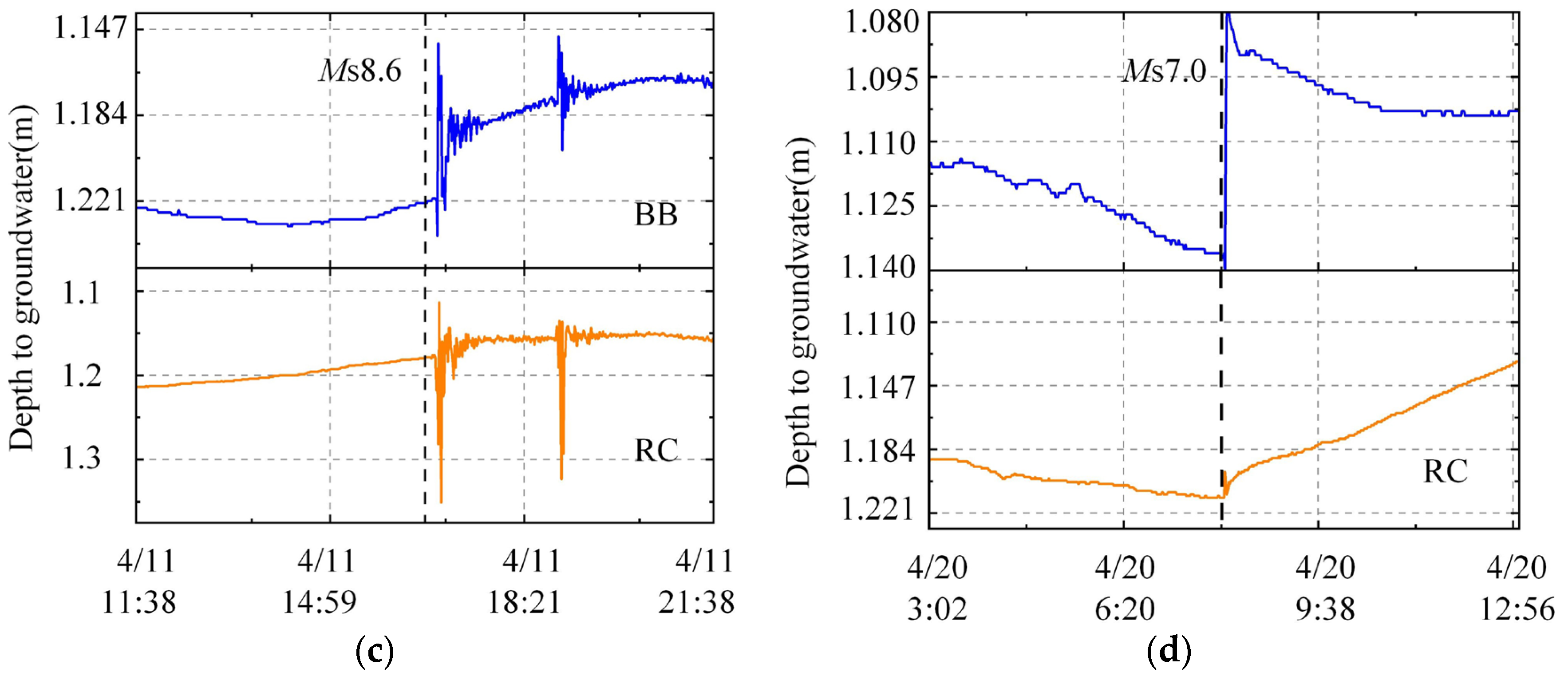
2.2. Response of Well Water Level to Multiple Earthquakes

This study collected minute observations of water levels in wells BB and RC from 2008 to 2016, and statistically found that both wells responded significantly to four strong earthquakes with magnitudes above Ms7.0 (

Table 1. Detailed information of four selected earthquakes.

Earthquake	Date	Time	Latitude (°N)	Longitude (°E)	Depth (km)	Magnitude (Ms)
Wenchuan	12 May 2008	14:28	103.4	30.9	33	8.0
Lushan	13 April 2013	08:02	103.0	30.3	13	7.0
Tohoku	11 March 2011	13:46	42.6	38.1	20	9.0
Sumatra	11 April 2012	16:38	93.1	2.3	20	8.6

). During the Wenchuan earthquake, the water level in well BB displayed a noticeable co-seismic step-down change, with a drop of approximately 95 cm, followed by a slow recovery after 3 h to 1.345 m after 45 d (compared to 1.19 m before the earthquake), with subsequent observation data missing. Comparatively, the water level in well RC co-seismically dropped by about 92 cm and quickly returned almost to the pre-earthquake level within 3 h of the earthquake (Figure 2a). The Tohoku earthquake caused an 8 cm step-up in the water level of well BB, accompanied by oscillations, and did not show any significant recovery characteristics 1 d after the earthquake. But the water level in well RC oscillated with an amplitude of 45 cm, and returned to a stable state within 2 h of the earthquake (Figure 2b). The Sumatra earthquake resulted in a 3.2 cm step-up followed by oscillations of 9 cm amplitude in the water level of well BB, with no significant post-seismic recovery. The water level in well RC also oscillated with an amplitude of 23.8 cm, but recovered to the pre-earthquake level within half an hour (Figure 2c). Finally, the Lushan earthquake caused a 5.4 cm step-up in the water level of well BB, only recovering to 30% of its pre-earthquake level within 5 h of the earthquake. The water level in well RC exhibited a 1.3 cm pulse-up change, returning to its pre-earthquake level within a few minutes (Figure 2d).

Overall, the recovery process of the water level in well BB is relatively slower after the earthquake, while the recovery process of well RC is shorter. Taking the Wenchuan earthquake as an example, the co-seismic water level in both wells dropped dramatically, and well BB had not entirely recovered 45 d after the earthquake, whereas well RC had nearly recovered within just 3 h. Wells BB and RC have similar tectonic and hydrogeologic conditions, but the recovery time in well RC is significantly lower than that in well BB after the earthquake. This study utilized the Wenchuan earthquake as an example to simulate and investigate the possible reasons for the co-seismic similarity and post-seismic variability in well water levels.

3. Methods

3.1. Fault Rupture Model

Roeloffs and Wang considered that an epicenter of 1–2 fault rupture lengths can be considered a near field [4,35]. The Wenchuan earthquake occurred in the Longmenshan fault zone in Sichuan Province, with the epicenter at a distance of 326 km and 271 km of wells BB and RC, respectively. Based on a criterion of the two times the fault rupture lengthens, both wells are within the near field. So, the Okada semi-elastic spatial dislocation theory was employed to establish the seismic rupture model and estimate the stress–strain generated by the focal fault rupture. The Okada dislocation model assumes that the Earth is elastic with no surface stress, neglects gravity, magnetism, curvature, temperature, and inhomogeneity, and considers the fault in a semi-infinite space with the surface as the boundary, and the strain value at infinity is zero. The USGS developed the software Coulomb 3.3, which is based on the Okada semi-elastic spatial dislocation model. The spatial distribution characteristics of the co-seismic stress–strain created by focal fault rupture may be determined using some basic earthquake data, such as the hypocenter’s coordinates and the geometrical dimensions of the focal rupture.

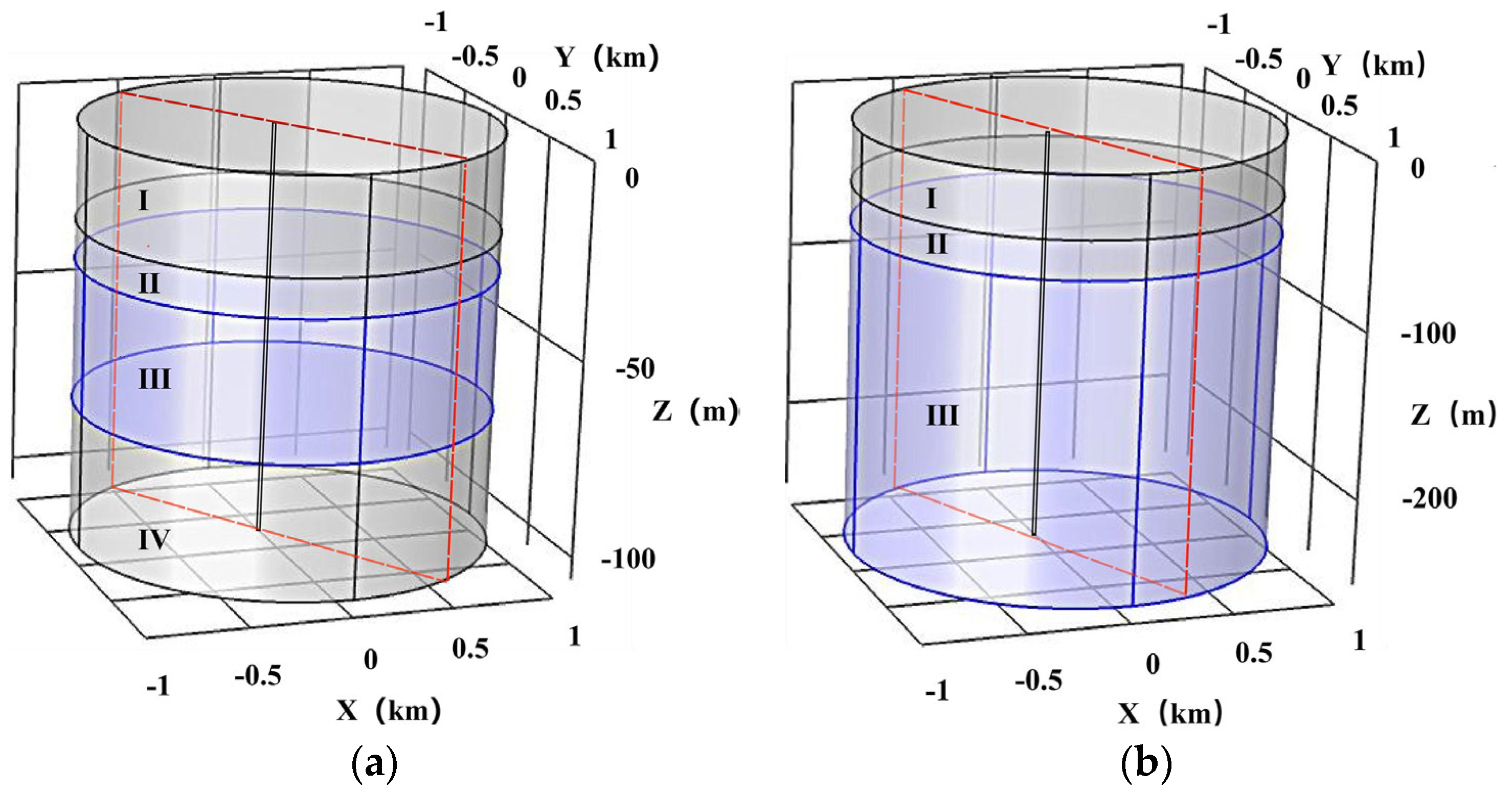
3.2. Numerical Modeling of Pore Pressure Response

The Wenchuan earthquake causes the stress and strain changes in the aquifer in the study area, the coupling of elastic deformation and pore pressure fluctuations in the porous medium will result in the changes in well water levels, and this study established a numerical model to characterize the pore pressure response due to the Wenchuan earthquake. According to the hydrogeological conditions, geological structure, wellbore characteristics, and so on, a 3D geometric model of the borehole–aquifer system was constructed. Based on the theories of Darcy’s law, Hooke’s law, mass conservation law, momentum conservation law, and Terzaghi’s law, the governing mathematical equations of fluid-solid coupling were established for the response of pore pressure to seismic stress. Employing the solid mechanics and Darcy’s law modules in the simulation software COMSOL Multiphysics, the process of pore pressure response of the observed aquifer to earthquakes was simulated using the finite element method by setting the initial conditions, boundary conditions and aquifer parameters.

It is assumed that the groundwater movement conforms to Darcy’s law, the layer is a homogeneous isotropic elastic porous medium, which satisfies the theory of pore linear elasticity, and the fluid is compressible. Moreover, the tension is ruled as positive and compression as negative, and the effects of temperature are ignored. Then, the process of the pore pressure changes (p) driven by seismic stress (σ) can be described by the following fluid–solid coupling governing equations:

$$\left\{\begin{array}{l}{\nabla }^2{\sigma }_{kk}+{\displaystyle \frac{2(1-2\nu )}{1-\nu }}\alpha {\nabla }^{2}p=0\\ \nabla k({\displaystyle \frac{\nabla p}{\rho g}}+\nabla z)=S_s{\displaystyle \frac{\partial p}{\rho g\partial t}}+\partial {\displaystyle \frac{\partial {{\displaystyle \epsilon }}_{kk}}{\partial t}}\end{array}\right.$$

(1)

where the stress–strain (σ–ε) follows Hooke’s law; ρ $(\mathrm{kg}·{\mathrm{m}}^{-3})$ represents the fluid density and g $(\mathrm{m}·{\mathrm{s}}^{-2})$ denotes the gravitational acceleration; ν is the Poisson’s ratio; k $(\mathrm{m}·{\mathrm{s}}^{-1})$ is the hydraulic conductivity; ${\nabla }^2$ is the Laplace operator, defined as ${\nabla }^2={\displaystyle \frac{{\partial }^2}{\partial x^2}}+{\displaystyle \frac{{\partial }^2}{\partial y^2}}+{\displaystyle \frac{{\partial }^2}{\partial z^2}}$; α is the effective stress coefficient, given by $\alpha =1-K/K_s$, where K and K_s are the bulk modulus of the porous medium and the solid particles, respectively; $S_s$ is the specific storativity, expressed as $S_s=\rho g(n{\displaystyle \frac{1}{K_f}}+(1-n){\displaystyle \frac{1}{K_s}})$, where K_f is the bulk modulus of fluid and n is the porosity; z is the height.

The strain ($\mathsf{\Delta }{\epsilon }_{kk}$) induced by the Wenchuan earthquake needs to be converted into the corresponding stress ($\mathsf{\Delta }{\sigma }_{kk}$) and applied to the aquifer. The relationship between them can be expressed as $\mathsf{\Delta }{\sigma }_{kk}=K_u\mathsf{\Delta }{\epsilon }_{kk}$, $K_u={\displaystyle \frac{2G(1+\nu )}{3(1-2\nu )}}$, G represents the shear modulus, K_u denotes the bulk modulus of the porous medium under undrained conditions.

4. Results

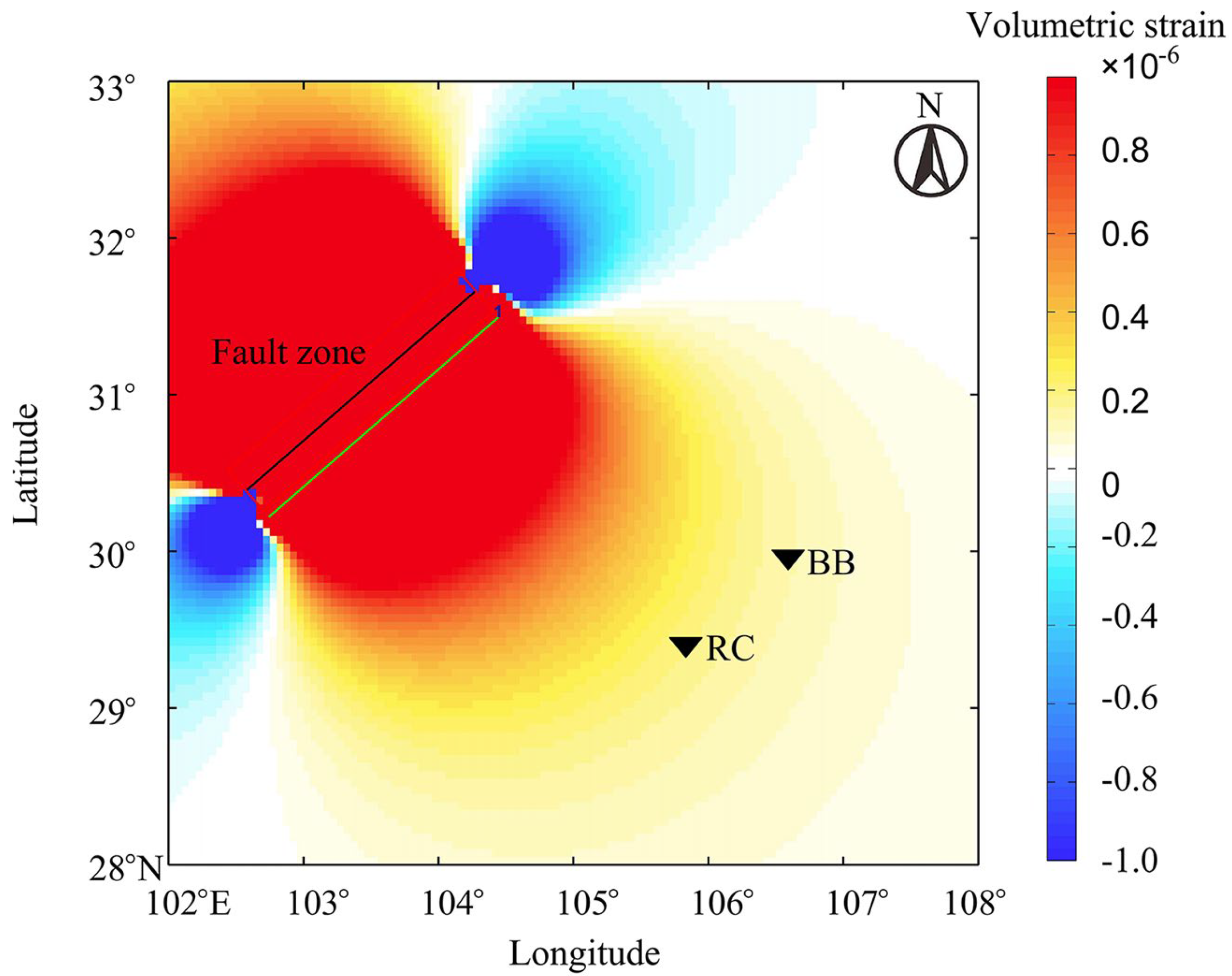
4.1. Seismic Stress–Strain Field

Table 2. The parameters of focal fault rupture for the Wenchuan earthquake.

Parameter	Value
Longitude range (°E)	102–108
Latitude range (°N)	28.0–33.0
Warp and weft mesh division accuracy (°)	0.05
Surface wave magnitude	8.0
Fault zone length (km)	216
Fault zone width (km)	45
Fault zone depth (km)	15.4
Move towards (°)	229
Dip angle (°)	32
Mean slip angle (°)	100
Poisson’s ratio	0.25

shows the basic information of the Wenchuan earthquake [36], and the spatial distribution of the co-seismic strain field generated by focal fault rupture was obtained by the software Coulomb 3.3 (Figure 3). The overall characteristics of the site stress–strain obtained are basically consistent with the results of Shi and Yang [21,37]. The findings show that the strain tension and compression regions caused by the Wenchuan earthquake have a characteristic of four-quadrant distribution, with extreme values distributed on both sides of the rupture with an order of magnitude of 10⁻⁶, and strain values gradually decreasing away from the rupture region. As shown in Figure 3, both BB and RC are subjected to tension.

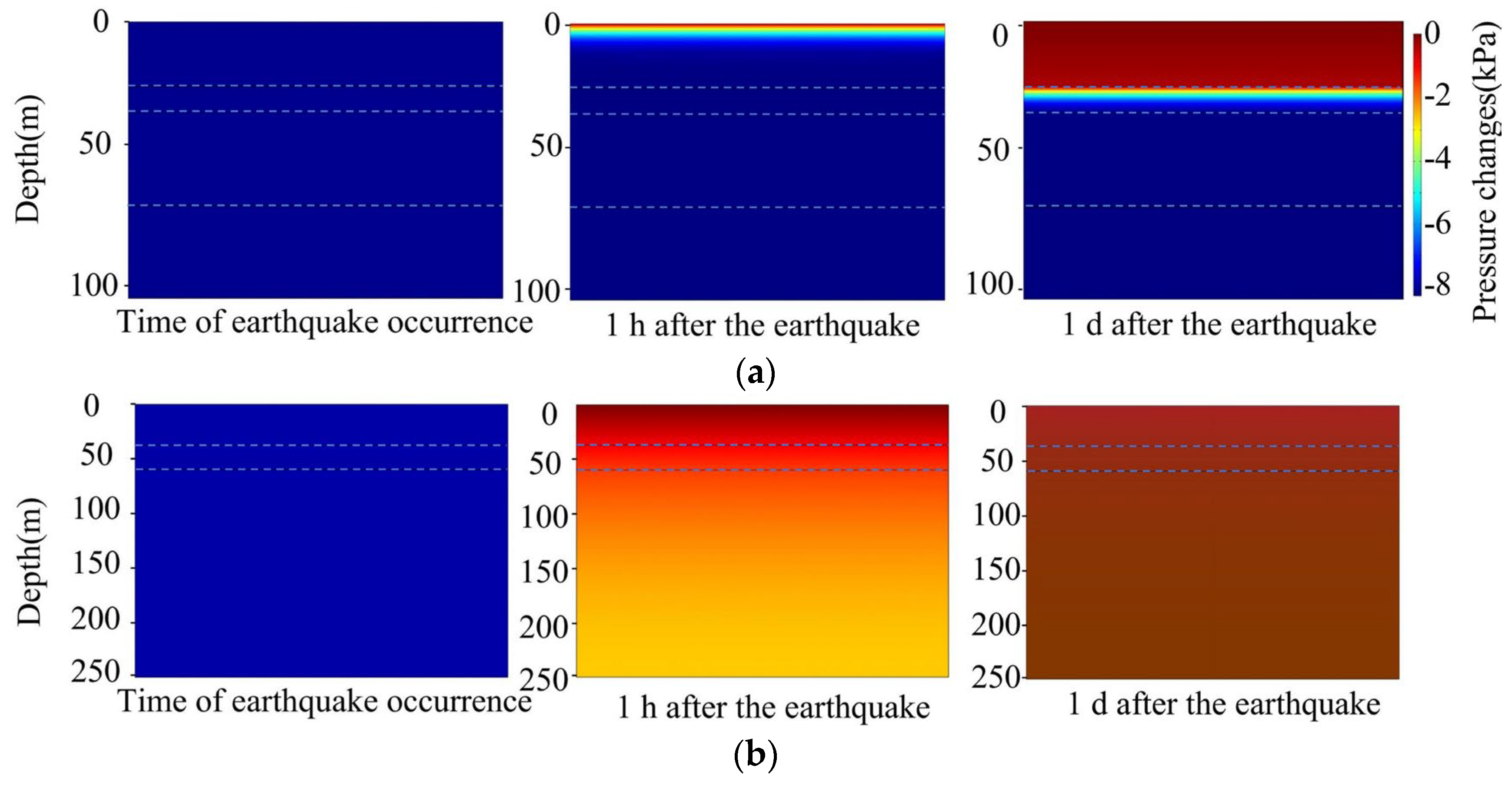
4.2. Results of Numerical Simulation

Figure 4 depicts the geometrical models of BB and RC aquifer systems, with the simulated area being a 1 km radius region centered on the observation wells, with depths of 105.6 m and 251.0 m, respectively, and the generalized stratigraphic structure and parameters are shown in

Table 3. Structure and parameters of the generalized stratigraphy of wells BB and RC.

BB
Layer	Lithology	Depth (m)	Density (kg/m3)	Hydraulic Conductivity (m/s)	Porosity	Poisson’s Ratio	Young’s Modulus (Pa)
I	Mud	0–30	1700	1.0 × 10−6	0.35	0.35	5 × 106
II	Crystal filling	30–40	2200	3.0 × 10−7	0.25	0.25	5 × 108
III	Sand	40–71	2000	3.0 × 10−6	0.30	0.30	5 × 107
IV	sandy mudstone	70–105.6	1850	2.0 × 10−6	0.32	0.30	3 × 107
RC
Layer	Lithology	Depth   (m)	Density (kg/m3)	Hydraulic conductivity (m/s)	Porosity	Poisson’s ratio	Young’s modulus (Pa)
I	Shale	0–37	1800	1.0 × 10−6	0.35	0.35	6 × 106
II	Sand	37–60	2000	2.5 × 10−6	0.32	0.3	3 × 107
III	Sand	60–251	2000	3.0 × 10−6	0.30	0.3	5 × 107

[38]. The upper boundary is set as a free boundary and there is no flow at the lower and surrounding boundaries. In addition, there is no horizontal displacement at the surrounding boundary and no vertical displacement at the lower boundary. Due to the complexity and effort of solving the mathematical governing equations, the finite element software COMSOL is employed to calculate the co-seismic and post-seismic sustained changes in the pore pressure. A free trihedral mesh is utilized for spatial sectioning, and to ensure accuracy, the time step for model BB is 1 h in 0–1 d and 1 d after that, while it is 1 h for model RC. The simulation time is set to 60 d for model BB and 3 h for model RC, ensuring that the pore pressure recovered to over 90%.

Figure 5 displays the 2D radial profiles of pore pressure changes generated by seismic stress near wells BB and RC, with the earthquake resulting in a transitory drop in pore pressure of around 80 kPa. Within 1 h of the earthquake, there were almost no changes in well BB, except for a clear recovery at depths of 0–8 m, while well RC had recovered by 75%. Within 1 d of the earthquake, there was still no significant recovery of pore pressure in well BB, but well RC had almost recovered, and it is clear that the recovery rate of pore pressure in well BB is significantly slower than that in well RC after the earthquake. Figure 6 depicts the characteristics of the pore pressure at different times and depths on the 2D profile. For well BB, it is found that the recovery rate of pore pressure varies in different layers (Figure 6a). The pore pressure at depths of 0–40 m (layers I and II) recovers more rapidly, and the shallower the depth, the faster the recovery; for example, at a depth of 30 m, it takes 30 d to recover, whereas near the surface, it takes just one day. The pore pressure at depths of 40–105.6 m (layers III and IV) is relatively slow to recover, with about 93% recovery 60 d after the earthquake, and there is no significant difference in the recovery time and rate with depth. For well RC, the pore pressure of layers I~III can be restored quickly within 3 h (Figure 6b), whereas the pore pressure at depths of 0–37 m (layer I) can be recovered more rapidly, with complete recovery in 1 h, and the pore pressure at depths of 37–251 m (layers II and III) can be recovered by more than 99% in 3 h, which is relatively slow.

5. Discussion

5.1. Comparison Between the Simulated and Measured Values

According to the dislocation model, the Wenchuan earthquake resulted in a clear four-quadrant distribution of crustal stress–strain in the study area, with the well water level rising co-seismically in the compression zone, and falling in the tension zone. Wells BB and RC are located in the tension zone, and the observed data show that the water levels in both wells exhibit obvious decreasing co-seismically, which is consistent with the calculation results of the dislocation, indicating that the co-seismic changes in the well water levels are mainly controlled by the tectonic stress generated by focal fault rupture. According to $p=\rho gh$, the changes in pore pressure caused by the earthquake are converted into the well water level. Figure 7 compares the measured and simulated water level in wells BB and RC; they both exhibit the characteristics of co-seismic step-down followed by recovery. The maximum simulated amplitude of water level in well BB is 83 cm, which basically recovered within 60 d of the earthquake. The maximum amplitude of the water level in well RC is 81 cm, which basically recovered within 3 h. The simulated trends in both well water levels are basically consistent with the measured, but there is a slight difference in the maximum amplitude of the water level. The measured amplitude of water level in wells BB and RC is 95 cm and 93 cm, respectively, which is greater than the simulated values. Four evaluation indexes, including Nash efficiency coefficient (NSE), root mean square error (RMSE), volume efficiency (VE) and standardized residual ratio (RSR), were used to evaluate the accuracy and reliability of the numerical simulation results [39,40,41]. The NSE, RMSE, VE and RSR of BB well were 0.65, 0.148, 7% and 0.58, respectively, and the NSE, RMSE, VE and RSR of RC well were 0.63, 0.150, −28% and 0.60, respectively. It shows that the numerical model can effectively reflect the general change trend of the water level of the two wells, and the calculated results are reliable. However, earthquake-induced water level changes are usually abrupt, often accompanied by high-frequency noise and abrupt values, often with multiple aftershocks, and subject to site effects, which can produce some errors.

Earthquake-induced changes in the well water level are affected by multiple factors such as seismic stress, the characteristics of wellbore–aquifer system [9,42], and so on. So, the process and morphology are complex and diverse, and earthquakes may also lead to changes in aquifer parameters, such as Skempton parameter, porosity, hydraulic conductivity, and so on [5,14]. Using the Okada dislocation theory to calculate the seismic stress–strain values generated also does not take account the effects of regional tectonic conditions and aquifer heterogeneity, which may result in errors between the simulated and actual values of the water level. Furthermore, taking well BB as an example, although the trend of the post-seismic continuous changes in water level is consistent with the observed, it is obvious that there are many abrupt small-amplitude changes in the observed water level. A series of aftershocks occurred after the Wenchuan earthquake, and through comparison, it is found that the abrupt small-amplitude changes in the measured water level in well BB are basically consistent with the aftershocks, and it is obvious that this change characteristic is closely related to the adjustment of the aquifer to the aftershock stress, but the performance of well RC is not significant. At the same time, the observed water level can clearly exhibit the obvious tidal response characteristics of one peak and one valley, or two peaks and two valleys. It cannot be ruled out that the well water level is affected by external loads such as barometric pressure precipitation and other external loads; so, there will be some deviation between the simulated and the measured water level. But, overall, the simulation results can reflect the response process of the well water level to the earthquake.

5.2. Determination of Aquifer Confinement

The lithology of the observed aquifers in both BB and RC is sandstone, and the strain values generated by the Wenchuan earthquake is 10 × 10⁻⁷ orders of magnitude, and the water levels in both wells show a similar co-seismic step-down, with amplitudes of 83 and 81 cm, respectively. However, there are significant differences in the continuous changes after the earthquake, and the pore pressure of wells BB and RC recovered within 60 d and 3 h, respectively. By comparing the histograms of the two wells, it can be seen that the fractures at 30–40 m depth in well BB are filled with calcite and pyrite minerals, the hydraulic conductivity is relatively poor, and the groundwater movement between adjacent layers is restricted. The aquifer in well RC is overlain by fine sandstone and shale with developed fissures, and is subjected to torsional stress, relatively weak confinement, and good interlayer hydraulic exchange. Could this be the reason for the difference in the sustained water level changes in both wells? The spectral analysis of the well water level is used to further determine the difference in the confinement of the observed aquifer near the two wells.

The frequency spectrum data of well water levels often contain multiple tidal signals, among which the primary tidal signals are M2, K1, S2, and O1 waves. These signals provide critical references for assessing aquifer confinement [42,43]. In an ideal unconfined aquifer, where the groundwater is connected to atmosphere, no tidal signals will be detected in the spectral analysis [44]. But, in fact, an unconfined aquifer is often overlain by an aeration zone, resulting in a signal lag effect, which that may generate S₂ and K₁ waves. In a confined aquifer, due to the limitation of the overlying confining layer, the barometric effect is not significant and it is mainly affected by the Earth tide; therefore, the M₂ wave dominates and other signals are also detected [45]. A semi-confined aquifer is weakly confined and has an obvious barometric effect, with S₂ dominating signals and the M₂ wave still being present [46]. Here, we focus on the period from 21 September 2007 to 24 November 2009, during which well water levels responded significantly to barometric pressure and Earth tidal fluctuations. The spectrum analyses of the groundwater level, barometric pressure and Earth tide were performed for wells BB and RC (Figure 8). The results show that all four tidal components are present in well BB and that the M₂ wave dominates, indicating that the aquifer is well confined (Figure 8a). However, the main components of the RC well water level are S₂ and K₁ waves, and the S₂ wave dominates (Figure 8b), which indicates that the aquifer is more affected by barometric pressure and it is weakly confined. So, the confining condition of well BB is obviously better than that of well RC.

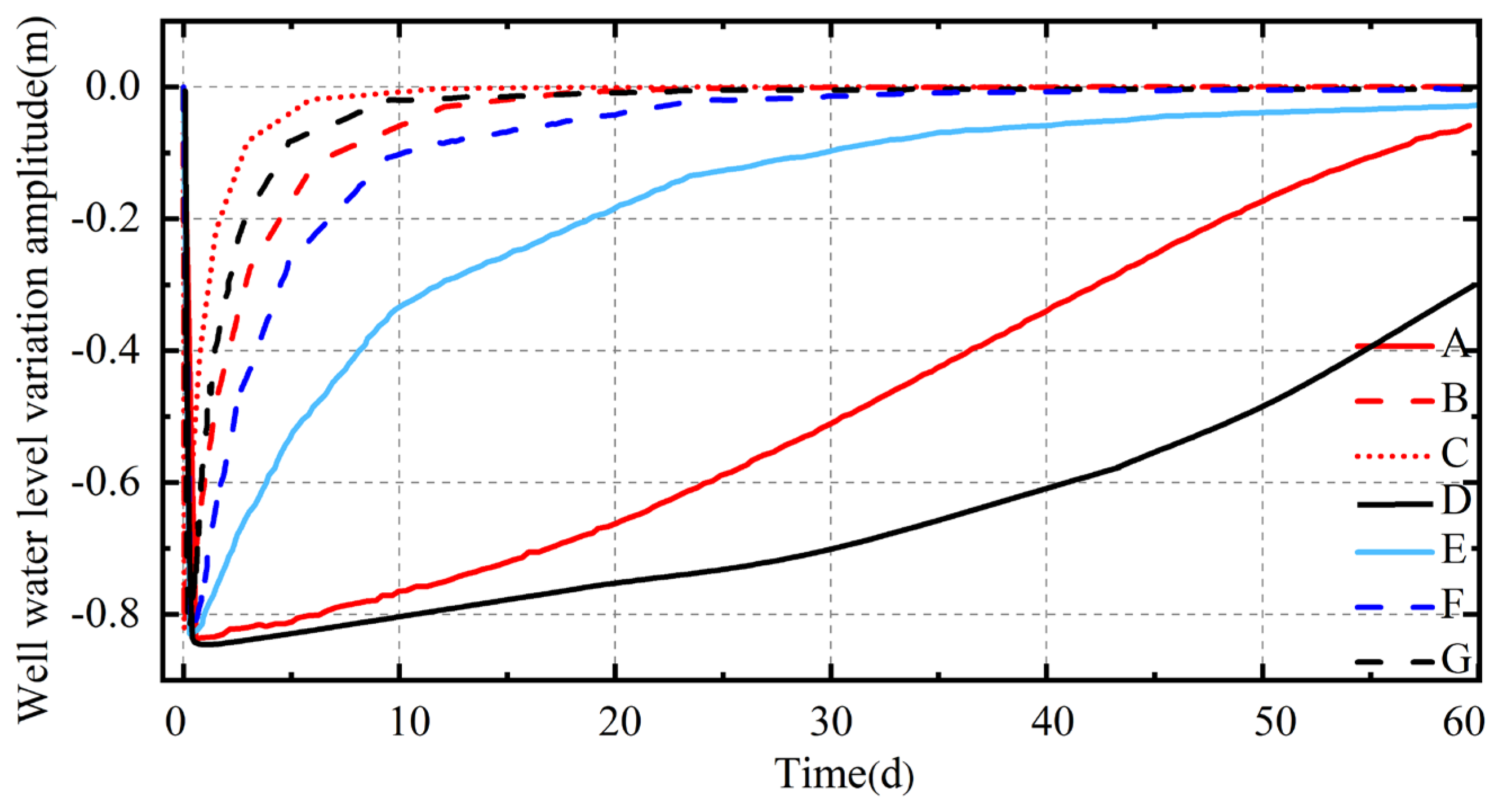
5.3. The Impact of Confinement on the Continuous Change in Well Water Level

Taking well BB as an example, the confinement of the observed aquifer is changed by increasing or decreasing the hydraulic conductivity and thickness of the overlying layer (II). With the help of the software COMSOL, the response characteristics of the well water level under different scenarios were calculated and the influence of aquifer confinement on the continuous change in the well water level was explored (Figure 9). The different scenarios are shown in

Table 4. Hydraulic conductivity and thicknesses of confining layers for different scenarios.

Scenario	Hydraulic Conductivity (m/s)	Thickness (m)
Case A	3.0 × 10−7	10
Case B	3.0 × 10−6	10
Case C	3.0 × 10−5	10
Case D	3.0 × 10−7	20
Case E	3.0 × 10−7	5
Case F	3.0 × 10−6	20
Case G	3.0 × 10−6	5

, and other parameters and conditions of the aquifer are constant.

The numerical simulation results show that, although the hydraulic conductivity and thickness of the confining layer of the observed aquifer are adjusted, the magnitude of the pore pressure and the well water level during the earthquake are still 8 kPa and 83 cm, respectively, which is basically the same as in the previous simulation results, indicating that the co-seismic changes in well water levels are mainly controlled by the stress–strain generated by focal fault rupture. But there is still a significant difference in the recovery process after the abrupt change, as the recovery time of well water level is 60 d in case A, 10 d in case B, and 5 d in case C. Comparing the simulation results of case A~B~C, it can be seen that when the hydraulic conductivity increased by one order of magnitude, the recovery time of the well water level is shortened by several times, i.e., when the observed aquifer is not overlain by the confining layer with poor hydraulic conductivity, both pore pressure and well water level are easy to recover in a very short time. In case D, the well water level decreased by 31 cm in 60 d, and only 62% recovered, while in case E, 90% was recovered in 40 d. Comparing the simulation results of case A~D~E, it can be seen that when the thickness of the confining layer with lower hydraulic conductivity decreases, the recovery time of the well water level becomes shorter. Meanwhile, the recovery time of the well water level is 15 d for case F and 8 d for Case G. Comparing the case B~F~G, it is clear that when the hydraulic conductivity of the confining layer is higher, the recovery time of the well water level is shortened with the smaller thickness of the layer, but not as significant as that when the hydraulic conductivity of the confining layer is lower. Although both the thickness and hydraulic conductivity of confining layer will affect the sustained changes in well water levels after the earthquake, the changes are more sensitive to the hydraulic conductivity.

The observed aquifer in well RC is almost sandstone, and although there is a very thin layer of shale sandwiched by a thin coal seam, the fractures in this layer are more developed and the permeability of the coal seam is better. The existing data also indicate that the northeast section was twisted to make the regional stress concentration, resulting in more developed fissures in the formation, and there may be some fissure channels connected with the atmosphere [47]. And spectral analysis further proves that well RC is poorly confined, more obviously affected by barometric pressure, and has active hydraulic exchange, which may be one of the reasons why the water level in well RC was able to recover rapidly after the Wenchuan earthquake.

6. Conclusions

Wells BB and RC are located in the near field of the Wenchuan earthquake, and the changes in pore pressure and well water level are mostly consistent with four-quadrant distribution of seismic stress, with the water level characterized by co-seismic step-down followed by recovery. The numerical simulation can accurately duplicate the entire response process of the well water level to an earthquake, and the simulated values are generally consistent with the measured ones. However, because of the changes in aquifer parameters, the impact of aftershocks and the effects of external loads such as Earth tide, barometric pressure and precipitation are not considered in the simulation process, the details of the well water level response to the earthquake are not accurate enough, and the simulated curves still have a certain degree of deviation from the observed ones.

The observed aquifer of well BB is overlain by the mudstone layer with low hydraulic conductivity, which is impacted by calcite and pyrite fillings at depths of 30 m and 43 m, respectively, and the groundwater transfer between adjacent layers is relatively slow. Meanwhile, the observed layer of well RC is overlain by fine sandstone and shale with fissures, and is subjected to torsional stress, indicating that the aquifer is weakly confined, as supported by spectral analysis. Numerical simulations reveal that the recovery time of pore pressure is shortened by several times when the hydraulic conductivity of the confining layer increases by one order of magnitude or the thickness decreases. Confinement plays an important role in the response time of well water levels after the earthquake, which may also explain the changes in BB and RC well water levels within 60 d and 3 h after the earthquake, respectively. There are other factors influencing the seismic response characteristics of well water level, such as tectonic conditions, well wellbore structure and aquifer parameters, and so on. However, because wells BB and RC are so close to each other near the Huayingshan fault zone, and the lithology of both observed aquifers is sandstone, the influence of aquifer confinement on the seismic effect of well water level is primarily examined in this study.

References

1. Bower, D.R.; Heaton, K.C. Response of an Aquifer near Ottawa to Tidal Forcing and the Alaskan Earthquake of 1964. Can. J. Earth Sci. 1978, 15, 331–340. [Google Scholar] [CrossRef]
2. Del Gaudio, E.; Stevenazzi, S.; Onorati, G.; Ducci, D. Changes in Geochemical and Isotopic Contents in Groundwater before Seismic Events in Ischia Island (Italy). Chemosphere 2024, 349, 140935. [Google Scholar] [CrossRef]
3. Lan, S.; Chi, B.; Jiang, J. Comparison of Groundwater-Level Response to Near Earthquake and Distant Earthquake:Taking Wenchuan Earthquake and Sumatra Earthquake for Example. J. Jilin Univ. (Earth Sci. Ed.) 2011, 41, 145–152. [Google Scholar] [CrossRef]
4. Wang, C.; Manga, M. Hydrologic Responses to Earthquakes and a General Metric. Geofluids 2010, 10, 206–216. [Google Scholar] [CrossRef]
5. Wang, C.-Y.; Wang, C.-H.; Kuo, C.-H. Temporal Change in Groundwater Level Following the 1999 (M w = 7.5) Chi-Chi Earthquake, Taiwan. Geofluids 2004, 4, 210–220. [Google Scholar] [CrossRef]
6. Gong, H.; Liao, X.; Li, G.; Chen, M. Dynamic characteristics of water level tides of four wells in the Huayingshan area. Technol. Earthq. Disaster Prev. 2016, 11, 600–610. [Google Scholar]
7. Brace, W.F.; Paulding, B.W.; Scholz, C. Dilatancy in the Fracture of Crystalline Rocks. J. Geophys. Res. 1966, 71, 3939–3953. [Google Scholar] [CrossRef]
8. Wakita, H. Water Wells as Possible Indicators of Tectonic Strain. Science 1975, 189, 553–555. [Google Scholar] [CrossRef]
9. Jónsson, S.; Segall, P.; Pedersen, R.; Björnsson, G. Post-Earthquake Ground Movements Correlated to Pore-Pressure Transients. Nature 2003, 424, 179–183. [Google Scholar] [CrossRef] [PubMed]
10. Brodsky, E.E.; Prejean, S.G. New Constraints on Mechanisms of Remotely Triggered Seismicity at Long Valley Caldera. J. Geophys. Res. 2005, 110, 2004JB003211. [Google Scholar] [CrossRef]
11. Elkhoury, J.E.; Niemeijer, A.; Brodsky, E.E.; Marone, C. Laboratory Observations of Permeability Enhancement by Fluid Pressure Oscillation of in Situ Fractured Rock. J. Geophys. Res. 2011, 116, B02311. [Google Scholar] [CrossRef]
12. Sun, X.; Xiang, Y.; Shi, Z.; Wang, B. Preseismic Changes of Water Temperature in the Yushu Well, Western China. Pure Appl. Geophys. 2018, 175, 2445–2458. [Google Scholar] [CrossRef]
13. Wang, C.; Chia, Y. Mechanism of Water Level Changes during Earthquakes: Near Field versus Intermediate Field. Geophys. Res. Lett. 2008, 35, 2008GL034227. [Google Scholar] [CrossRef]
14. Liao, X.; Wang, C.; Liu, C. Disruption of Groundwater Systems by Earthquakes. Geophys. Res. Lett. 2015, 42, 9758–9763. [Google Scholar] [CrossRef]
15. Sturtevant, B.; Kanamori, H.; Brodsky, E.E. Seismic Triggering by Rectified Diffusion in Geothermal Systems. J. Geophys. Res. 1996, 101, 25269–25282. [Google Scholar] [CrossRef]
16. Zhang, H.; Shi, Z.; Wang, G.; Sun, X.; Yan, R.; Liu, C. Large Earthquake Reshapes the Groundwater Flow System: Insight from the Water-Level Response to Earth Tides and Atmospheric Pressure in a Deep Well. Water Resour. Res. 2019, 55, 4207–4219. [Google Scholar] [CrossRef]
17. Wang, C.-Y.; Manga, M. New Streams and Springs after the 2014 Mw6.0 South Napa Earthquake. Nat. Commun. 2015, 6, 7597. [Google Scholar] [CrossRef]
18. Faoro, I.; Elsworth, D.; Marone, C. Permeability Evolution during Dynamic Stressing of Dual Permeability Media. J. Geophys. Res. 2012, 117, 2011JB008635. [Google Scholar] [CrossRef]
19. Yan, R.; Woith, H.; Wang, R. Groundwater Level Changes Induced by the 2011 Tohoku Earthquake in China Mainland. Geophys. J. Int. 2014, 199, 533–548. [Google Scholar] [CrossRef]
20. Itaba, S.; Koizumi, N.; Toyoshima, T.; Kaneko, M.; Sekiya, K.; Ozawa, K. Groundwater Changes Associated with the 2004 Niigata-Chuetsu and 2007 Chuetsu-Oki Earthquakes. Earth Planets Space 2008, 60, 1161–1168. [Google Scholar] [CrossRef]
21. Shi, Z.; Wang, G.; Liu, C. Co-Seismic Groundwater Level Changes Induced by the May 12, 2008 Wenchuan Earthquake in the Near Field. Pure Appl. Geophys. 2013, 170, 1773–1783. [Google Scholar] [CrossRef]
22. Chia, Y. Changes of Groundwater Level Due to the 1999 Chi-Chi Earthquake in the Choshui River Alluvial Fan in Taiwan. Bull. Seismol. Soc. Am. 2004, 91, 1062–1068. [Google Scholar] [CrossRef]
23. Nespoli, M.; Todesco, M.; Serpelloni, E.; Belardinelli, M.E.; Bonafede, M.; Marcaccio, M.; Rinaldi, A.P.; Anderlini, L.; Gualandi, A. Modeling Earthquake Effects on Groundwater Levels: Evidences from the 2012 Emilia Earthquake (Italy). Geofluids 2016, 16, 452–463. [Google Scholar] [CrossRef]
24. Rojstaczer, S. Determination of Fluid Flow Properties from the Response of Water Levels in Wells to Atmospheric Loading. Water Resour. Res. 1988, 24, 1927–1938. [Google Scholar] [CrossRef]
25. Wang, C.-Y. Liquefaction beyond the Near Field. Seismol. Res. Lett. 2007, 78, 512–517. [Google Scholar] [CrossRef]
26. Weaver, K.C.; Cox, S.C.; Townend, J.; Rutter, H.; Hamling, I.J.; Holden, C. Seismological and Hydrogeological Controls on New Zealand-Wide Groundwater Level Changes Induced by the 2016 M w 7.8 Kaikōura Earthquake. Geofluids 2019, 2019, 9809458. [Google Scholar] [CrossRef]
27. Montgomery, D.R.; Manga, M. Streamflow and Water Well Responses to Earthquakes. Science 2003, 300, 2047–2049. [Google Scholar] [CrossRef] [PubMed]
28. Liu, C.-Y.; Chia, Y.; Chuang, P.-Y.; Chiu, Y.-C.; Tseng, T.-L. Impacts of Hydrogeological Characteristics on Groundwater-Level Changes Induced by Earthquakes. Hydrogeol. J. 2018, 26, 451–465. [Google Scholar] [CrossRef]
29. Weaver, K.C.; Arnold, R.; Holden, C.; Townend, J.; Cox, S.C. A Probabilistic Model of Aquifer Susceptibility to Earthquake-Induced Groundwater-Level Changes. Bull. Seismol. Soc. Am. 2020, 110, 1046–1063. [Google Scholar] [CrossRef]
30. Yan, R.; Wang, G.; Ma, Y.; Shi, Z.; Song, J. Local Groundwater and Tidal Changes Induced by Large Earthquakes in the Taiyuan Basin, North China from Well Monitoring. J. Hydrol. 2020, 582, 124479. [Google Scholar] [CrossRef]
31. Liao, X.; Wang, G.; Shi, Z. Sustained Changes in Well Water Levels Following a Large Earthquake: Possible Evidence of Permeability Decreases in a Shallow Groundwater System. Geophys. Res. Lett. 2021, 48, e2020GL090232. [Google Scholar] [CrossRef]
32. García-Gil, A.; Jimenez, J.; Gasco Cavero, S.; Marazuela, M.Á.; Baquedano, C.; Martínez-León, J.; Cruz-Pérez, N.; Laspidou, C.; Santamarta, J.C. Effects of the 2021 La Palma Volcanic Eruption on Groundwater Resources (Part II): Hydrochemical Impacts. Groundw. Sustain. Dev. 2023, 23, 100992. [Google Scholar] [CrossRef]
33. Dyer, G.B. Numerical Models of Fluid-Pressure Changes Resulting from the 1999 Chi-Chi Earthquake, Taiwan. Hydrogeology 2005, 543–551. [Google Scholar]
34. Wang, M.; Gu, H.; Liu, Q.; Wei, H.; Xu, Y.; Sauter, M. Seismically-Induced Groundwater Flow into Confining Clays: An Experimental and Numerical Study. J. Hydrol. 2024, 640, 131716. [Google Scholar] [CrossRef]
35. Roeloffs, E.A. Hydrologic Precursors to Earthquakes: A Review. Pure Appl. Geophys. 1988, 126, 177–209. [Google Scholar] [CrossRef]
36. Wang, W.; Zhao, L.; Li, J.; Yao, Z. Rupture process of the Ms8.0 Wenchuan earthquake of Sichuan. Chin. J. Geophys. 2008, 51, 1403–1410. [Google Scholar]
37. Yang, Z.; Deng, Z.; Yang, X.; Tao, J. Comparison and Analysis of Well Water-Level Variations Caused by Lusan Ms7.0 Earthquake In 2013 and Wenchuan Ms8.0 Earthquake in 2008. Seismol. Geol. 2014, 36, 380–391. [Google Scholar] [CrossRef]
38. Gong, H.; Li, G.; Li, C.; He, M.; Gao, J. Research on hydrogeological and hydrochemical environmental characteristics of Rongchang well. Seismol. Geomagn. Obs. Res. 2021, 42, 212–213. [Google Scholar] [CrossRef]
39. Yilmaz, K.K.; Gupta, H.V.; Wagener, T. A Process-based Diagnostic Approach to Model Evaluation: Application to the NWS Distributed Hydrologic Model. Water Resour. Res. 2008, 44, 2007WR006716. [Google Scholar] [CrossRef]
40. Alakbar, T.; Burgan, H.I. Regional Power Duration Curve Model for Ungauged Intermittent River Basins. J. Water Clim. Chang. 2024, 15, 4596–4612. [Google Scholar] [CrossRef]
41. Moriasi, D.N.; Gitau, M.W.; Pai, N.; Daggupati, P. Hydrologic and Water Quality Models: Performance Measures and Evaluation Criteria. Trans. ASABE 2015, 58, 1763–1785. [Google Scholar] [CrossRef]
42. Zhang, H.; Shi, Z.; Wang, G.; Yan, X.; Liu, C.; Sun, X.; Ma, Y.; Wen, D. Different Sensitivities of Earthquake-Induced Water Level and Hydrogeological Property Variations in Two Aquifer Systems. Water Resour. Res. 2021, 57, e2020WR028217. [Google Scholar] [CrossRef]
43. Turnadge, C.; Crosbie, R.; Barron, O. Comparing Methods of Barometric Efficiency Characterization for Specific Storage Estimation. Groundwater 2019, 57, 844–859. [Google Scholar] [CrossRef] [PubMed]
44. Rahi, K.A.; Halihan, T. Identifying Aquifer Type in Fractured Rock Aquifers Using Harmonic Analysis. Groundwater 2013, 51, 76–82. [Google Scholar] [CrossRef] [PubMed]
45. Bredehoeft, J.D. Response of Well-Aquifer Systems to Earth Tides. J. Geophys. Res. 1967, 72, 3075–3087. [Google Scholar] [CrossRef]
46. Weeks, E.P. Barometric Fluctuations in Wells Tapping Deep Unconfined Aquifers. Water Resour. Res. 1979, 15, 1167–1176. [Google Scholar] [CrossRef]
47. Gong, H.; Gao, X.; Yang, X.; Liang, H.; Xiang, Y.; Li, G. Precursory anomaly characteristics research of water radon based on M ≥ 5.0 earthquake case in China. Inland Earthq. 2016, 30, 168–176. [Google Scholar] [CrossRef]
Figure 1. (a) Geographical locations and (b) borehole structures of wells BB and RC, where the main observed aquifers are at depths of 30–71 m and 61–251 m, respectively.
Water 16 03484 g001
Figure 2. The co-seismic and sustained response of the water level in wells BB and RC during strong earthquakes—(a) the Wenchuan earthquake, (b) the Tohoku earthquake, (c) the Sumatra earthquake, and (d) the Ya’an earthquake.
Water 16 03484 g002aWater 16 03484 g002b
Figure 3. The spatial distribution characteristics of strain in the Wenchuan earthquake fault model. The blue color represents a negative volumetric strain, indicating that the region is subjected to compression, while the red color indicates a positive volumetric strain, indicating that the region is subjected to tension, and both BB and RC are in the tensile zone.
Water 16 03484 g003
Figure 4. Generalized 3D models of (a) BB and (b) RC aquifers; the blue area represents the observed aquifer, and the red line segment represents the simulated 2D radial profile.
Water 16 03484 g004
Figure 5. The pore pressure changes in 2D profile in wells (a) BB and (b) RC when the Wenchuan earthquake occurred, 1 h and 1 day after the earthquake. The positive and negative values indicate the increase and decrease in the pore pressure, respectively.
Water 16 03484 g005
Figure 6. Variation in pore pressure with time at different depths in wells (a) BB and (b) RC. The positive and negative values indicate the increase and decrease in the pore pressure, respectively.
Water 16 03484 g006
Figure 7. Comparison of the measured and calculated curves of water level response in wells BB (a) and RC (b) to the Wenchuan earthquake. The vertical coordinate represents only the magnitude of water level changes, and the blue arrows represent the aftershocks of the Wenchuan earthquake.
Water 16 03484 g007
Figure 8. Spectral analysis of groundwater level, barometric pressure, and Earth tide at wells (a) BB and (b) RC. For both wells, the barometric signal is mainly controlled by S2 and K1 waves, and the Earth tide is mainly controlled by M2, S2, O1 and K1 waves. For well BB, M2 and S2 waves dominate in the groundwater level signal, indicating that the aquifer is confined or semi-confined. For well RC, the S2 and K1 waves dominate in the groundwater level signal, and the aquifer is un-confined, with poor confining condition.
Water 16 03484 g008
Figure 9. The water level response in well BB under different cases A~G, the specific parameters are set as in Table 4. A represents the actual conditions; A, B and C represent the effect of different hydraulic conductivity of the confining layer on the well water level; A, D and E represent the effect of different thickness of the confining layer with lower hydraulic conductivity, and B, F and G represent the effect of the thickness of the confining layer with higher hydraulic conductivity.
Water 16 03484 g009