Towards Accurate Flood Predictions: A Deep Learning Approach Using Wupper River Data

Abstract

The increasing frequency and severity of floods due to climate change underscores the need for precise flood forecasting systems. This study focuses on the region surrounding Wuppertal in Germany, known for its high precipitation levels, as a case study to evaluate the effectiveness of flood prediction through deep learning models. Our primary objectives are twofold: (1) to establish a robust dataset from the Wupper river basin, containing over 19 years of time series data from three sensor types such as water level, discharge, and precipitation at multiple locations, and (2) to assess the predictive performance of nine advanced machine learning algorithms, including Pyraformer, TimesNet, and SegRNN, in providing reliable flood warnings 6 to 48 h in advance, based on 48 h of input data. Our models, trained and validated using k-fold cross-validation, achieved high quantitative performance metrics, with an accuracy reaching up to 99.7% and F1-scores up to 91%. Additionally, we analyzed model performance relative to the number of sensors by systematically reducing the sensor count, which led to a noticeable decline in both accuracy and F1-score. These findings highlight critical trade-offs between sensor coverage and predictive reliability. By publishing this comprehensive dataset alongside performance benchmarks, we aim to drive further innovation in flood risk management and resilience strategies, addressing urgent needs in climate adaptation.

1. Introduction

As a consequence of climate change, the occurrence of extreme weather events has increased on a global scale. This includes an increase in the frequency and intensity of heavy precipitation events, leading to a heightened risk of flooding [1]. It is crucial to acknowledge that floods are not only one of the most prevalent natural disasters but also one of the most devastating, resulting in significant economic losses, the destruction of infrastructure, and, regrettably, the loss of life [2]. The implementation of effective early warning systems is of critical importance in the mitigation of these risks. Such systems can provide essential lead time for communities and emergency managers to implement evacuation plans, deploy protective measures, and safeguard critical infrastructure.

For many years, traditional hydrological models have constituted the foundation of flood forecasting. These models can be complex, relying on extensive data inputs and intricate physics-based simulations. They have been in use for many decades [3] and provide water level forecasts for days and even weeks based on model architecture and allow the issuing of localized warnings.

However, their complexity, reliance on extensive data inputs, and intricate physics-based simulations often necessitate significant resources and expertise [4,5]. Moreover, these models may struggle to capture the inherent non-linear dynamics of short-term flood events. While many industrialized areas have the financial capacity to deploy and maintain complex hydrological warning systems, these solutions are not universally accessible [6]. As a consequence, there is a pressing need for more affordable and adaptable approaches that can provide reliable flood forecasting in diverse settings.

In addition to such simulation-based forecasting, the rapid development of data-based prediction models based on deep learning is leading to the emergence of complementary and alternative options. The efficacy of such deep learning models in recognizing complex patterns in large datasets has been demonstrated in a variety of applications. Consequently, they are suitable for analyzing the interplay of meteorological, hydrological, and geographical factors that influence flooding and may be implicitly mapped in sensor measurements such as precipitation, water levels, and discharges. Deep learning models are adept at identifying intricate patterns within large datasets, making them ideal for analyzing the interplay of meteorological, hydrological, and geospatial factors that influence flooding and are possibly implicitly depicted in sensor measurements like rainfall, water levels and discharges. As demonstrated by Kumar et al. [7] and Bentivoglio et al. [8], deep learning can offer a valuable approach to flood forecasting.

Deep learning models typically require less upfront investment compared to traditional methods. This is because they can be developed without expensive hydrological software, and their computational costs are primarily concentrated in the training phase. Furthermore, once trained, deep learning models are computationally efficient for generating predictions, reducing the ongoing operational burden. Finally, the ability to retrain and update deep learning models as environmental conditions change offers flexibility to adapt to evolving landscapes. The classical disadvantages of deep learning-based methods are a potentially time-consuming training phase to adjust a model to the training data, and the necessity for the careful selection and curation of the training data itself. This is due to the fact that the model can perform poorly if the training data are of low quality or only contain a few examples of interesting behavior (such as flood events) that have to be learned. Another disadvantage of most modern deep learning models is the lack of transparency of predictions. This means that the features and characteristics leading to the prediction are neither transparent nor comprehensible. This problem is being investigated in the relatively new research area of explainable AI, where solutions for creating comprehensibility and transparency are being researched.

By leveraging their ability to extract meaningful insights from sensor data, even with a limited number of stations, deep learning models can potentially achieve effective flood forecasting with a reduced number of monitoring stations, leading to significant cost savings on infrastructure.

Our research focuses on the Wupper river basin in Germany, a region characterized by diverse topography, multiple dams, and intense yearly rainfall patterns. This unique environment serves as an ideal testbed for evaluating the potential of deep learning models in flood forecasting. By leveraging two decades of comprehensive rainfall and water level data from the Wupper river, we aim to demonstrate the viability of a deep learning-based approach for reliable flood warning in a flood-threatened region.

In this paper, we provide the following main contributions:

• We compile a unique dataset spanning 19 years, including rainfall measurements and water level data from the Wupper river in Germany [9].
• We conduct a thorough assessment of state-of-the-art deep learning models specifically tailored for time-series analysis. Nine state-of-the-art deep learning models (such as Pyraformer, Informer and TimesNet) are compared on a classification task to issue warning forecasts in case of flood events in the near future. This benchmarking on real-world flood events offers crucial insights into model suitability and performance in issuing timely warning forecasts, a vital step toward reliable flood early warning systems.
• We study the effect of strongly reduced sensor numbers on the model performance, offering a novel estimate of the minimum sensor count necessary for reliable flood forecasting.

2. Related Work

With the ever-increasing number of floods not only in Germany but in many other countries worldwide, a great deal of work has been put into the early detection of floods. Traditional hydrological models for flood prediction and warning, leveraging a variety of different data inputs, are still in use and under research today. Nevertheless, a growing number of deep learning solutions are being researched and developed, complementing or replacing the often expensive and labor-intense traditional approaches.

2.1. Traditional Flood Forecasting Models

In their review, Jain et al. [10] evaluate large-scale hydrological models for operational flood forecasting, focusing on those suitable for the European Flood Awareness System (EFAS). The authors suggest that developing adaptable, high-performance models remains a key area for future research to improve operational forecasting efficiency and accuracy. Kauffeldt et al. [11] review large-scale hydrological flood forecasting models, each with distinct applications, strengths, and limitations. Deterministic models leverage physical laws for accuracy, while data-driven methods like neural networks analyze historical patterns. The authors also highlight the need for computationally efficient models that adapt to changing catchment conditions and allow rapid forecast updates to strengthen flood preparedness efforts.

The review, written by Jehanzaib et al. [12], provides a quick overview over runoff models. Runoff models calculate how much precipitation enters rivers and streams as runoff instead of seeping into the ground or evaporating. They can be used to predict floods by analyzing various factors such as soil moisture, vegetation, and precipitation levels in order to identify potential floods and their extent in certain areas at an early stage. In their review, Jehanzaib et al. [12] differentiate between conceptual, empirical, and physical models, each varying in structure and their corresponding spatial processing.

• Conceptual models aim to represent the hydrological process using simplified components. Even though they use parameters that are partially based on physical understanding, they are generally calibrated with observed data. An example for a conceptual model is the Hydrologiska Byråns Vattenbalansavdelning (HBV) [13], which balances simplicity and physical realism, making it efficient for flood prediction, even with limited data.
• Empirical models are data driven, relying on statistical correlations between rainfall and runoff without the detailed consideration of physical processes. It is said they are best suited for areas with extensive historical data but limited environmental detail. Developed by Cronshey [14], the Soil Conservation Service Curve Number (SCS-CN) estimates runoff based on land use, soil type, and rainfall.
• Physical models, also known as deterministic models, use mathematical equations to simulate the physicals processes affecting runoff, such as infiltration and evaporation. The Soil and Water Assessment Tool (SWAT) [15] simulates the impact of land management practices on water, sediment, and nutrient yields in large watersheds, providing a framework to assess water resource changes.

Norbiato et al. [16] investigate a method to improve the accuracy of flash flood forecasts at ungauged locations using the Flash Flood Guidance (FFG) method and a model-based runoff threshold computation to improve hydrological models. Cannon et al. [17] examine the rainfall conditions that trigger debris flows and floods in recently burned areas in Colorado and California. The authors develop empirical Rainfall Triggering Index (RTI) thresholds to predict when such events are likely to occur, providing valuable information for emergency warning systems and response planning.

Hapuarachchi et al. [18] discuss the limitations of traditional methods and the improvements that have been made in recent years. One important development in flash flood forecasting has been the use of blended quantitative precipitation estimates (QPEs) and quantitative precipitation forecasts (QPFs), which combine information from radar, satellite, and gauge data.

Furthermore, Giannaros et al. [19] conduct a case study of a flash flood that occurred in Olympiada, North Greece on 25 November 2019. They further discuss that QPFs remain a significant challenge, especially for local-scale events.

These works show the benefits that hydrological models still provide. Their, at least partial, usage of sensor data and prediction of flood events makes their efforts comparable to our work. However the common problems of hydrological models remain, and they still suffer from lowered performance on local short-term events, which we demonstrate to alleviate by using machine learning algorithms.

2.2. Deep Learning Models

The latest review on deep learning models in hydrology, written by Zhao et al. [20], primarily discusses the various deep learning architectures employed for hydrological forecasting, including recurrent neural network (RNN), long short-term memory (LSTM), and convolutional neural network (CNN). In their work, Zhao et al. [20] focus on the underlying architectures (and their variations) of various deep learning models in regards to hydrological forecasting.

In contrast, the work of Kumar et al. [7] features a broader approach. It not only reviews deep learning models but also delves into the different challenges in flood forecasting, such as data accessibility, the interpretability of models, and their integration into other methodologies. Kumar et al. [7] categorize various tasks within this domain, including the following:

• Flood forecasting using RNN and LSTM networks for time-series prediction of rainfall, river flow, and flood occurrence;
• Flood susceptibility mapping and flood extent detection with CNN for spatial data analysis, such as satellite and remote sensing imagery;
• Synthetic data generation with Generative Adversarial Networks (GANs) to supplement datasets in regions with scarce real data;
• Feature extraction through autoencoders and Self-Organizing Maps (SOMs) for the dimensionality reduction and identification of critical flood-related features.

They also discuss the importance of uncertainty estimations and ethical considerations in flood management, offering a more holistic view of the state-of-the-art in this field.

While many studies concentrate on river flood prediction through the forecasting of water levels [21,22,23] and river discharge rates [24,25], our focus is directed towards the classification of significant flood-related events rather than just forecasting water levels.

A notable contribution comes from Kimura et al. [26], who introduced a flood prediction model integrating a CNN with transfer learning techniques to predict time-series water level data during flood events across different watersheds using hourly rainfall data and water level sensors as input.

Building upon this methodology, Sankaranarayanan et al. [27] devise a system that incorporates seasonal data, including rainfall intensity and temperature, to predict the probability of flooding before substantial increases in streamflow and water levels based on a neural network. Their approach demonstrates superior accuracy in forecasting floods across multiple districts in the Indian states of Bihar and Orissa.

Meanwhile, Zhao et al. [28] tackle the challenge of large-scale flash flood warnings (FFWs) in the mountainous and hilly terrains of China. Their research focuses on an LSTM model, comparing its performance with traditional methods like the RTI and FFG. Their findings reveal that the LSTM demonstrates superior accuracy, providing reliable flood warnings a day in advance based on daily precipitation and spatial hydrological features, with a hit rate (HR) of 0.84 and a false alarm rate (FAR) of 0.09.

Panahi et al. [29] develop two deep learning models, CNN and RNN, to perform a classification of flash floods in the Golestan Province, Iran. The models are trained using a geospatial database, which include historical flood data and several geo-environmental factors such as slope, aspect, altitude, topographic wetness index, proximity to rivers, rainfall, land use, and lithology.

2.3. Deep Learning for Time Series

In recent years, more work has been put into the development of sophisticated deep learning architectures, particularly those in the field of time series. A series of state-of-the-art deep learning time-series models relevant to our work is introduced shortly.

Lin et al. [30] introduce a novel RNN architecture named SegRNN, which excels in long-term time-series forecasting (LTSF) but is also applicable to tasks such as classification and anomaly detection. The SegRNN model employs two innovative strategies: segment-wise iterations on the input and parallel multi-step forecasting, combined with a gated recurrent unit (GRU) [31] for enhanced performance.

Transformers, originally developed for natural language processing (NLP) by Vaswani et al. [32], have also been adapted for time-series forecasting, demonstrating their versatility and efficacy in this domain as shown in the survey from Wen et al. [33].

One of the most noteworthy models from said survey is the Temporal Fusion Transformer (TFT) from Lim et al. [34]. The TFT is a model designed to capture both short-term and long-term temporal dependencies in time-series data. It uses a combination of attention mechanisms to handle variable time series, static covariates, and missing values. The model is particularly effective for multi-horizon forecasting tasks and provides interpretability by visualizing important features.

Similarly, Nie et al. [35] present a transformer architecture that uses a patching mechanism akin to segment-wise iteration, effectively capturing local semantics for improved time-series modeling. A advancement in this area is the non-stationary transformer proposed by Liu et al. [36]. They develop a framework that addresses the challenges of forecasting non-stationary time-series data, which are data where the statistical properties change over time. Additionally, the de-stationary attention module approximates attention without stationarization, allowing the model to capture inherent temporal dependencies more accurately.

Wu et al. [37] introduce TimesNet, which employs the concept of multi-periodicity to transform one-dimensional time-series data into two-dimensional tensors. This approach allows for the more accurate representation of intra- and inter-period variations. TimesNet has demonstrated superior performance in a range of time-series analysis tasks, including forecasting, imputation, classification, and anomaly detection.

In 2024, Liu et al. [38] presented the iTransformer; a model designed for time-series forecasting, leveraging the power of the transformer architecture. It excels in capturing long-range dependencies within time-series data through self-attention mechanisms and can handle variable-length input and output sequences.

A similar model is the Informer from Zhou et al. [39]. It uses a self-attention mechanism, optimized for long sequences, by employing a probabilistic sampling technique to reduce the computational burden. This enables the Informer to effectively capture long-term dependencies and patterns in the data while maintaining scalability and efficiency. Additionally, the Informer introduces a novel ’distillation’ process that further compresses the sequence length by iteratively aggregating key information, which enhances the Informer’s ability to handle large datasets and complex temporal relationships.

Other approaches (e.g., [40,41,42]) utilize a method called Time Series Decomposition [43]. Time-series decomposition is the process of breaking down a time series into three primary components: trend, seasonality, and residuals. The trend component captures the long-term direction of the series, the seasonal component reflects repeating short-term cycles, and a residual component accounts for random noise or irregularities. This decomposition helps to elucidate and model the underlying patterns in the data, thereby improving the accuracy and interpretability of forecasts.

The FEDFormer, invented by Zhou et al. [44], takes it a step further by not only using the decomposition but also enhancing the representation in the frequency domain. By focusing on frequency components, the FEDFormer can capture periodic patterns more effectively.

Liu et al. [45] propose a novel transformer architecture specifically designed for long-term time-series forecasting, called the Pyraformer. The key innovation lies in its ability to reduce the computational complexity traditionally associated with transformers, making it more efficient for processing long sequences. It also introduces a hierarchical pyramidal attention mechanism, which is used to downsample the input sequence, allowing for the capture of both local and global temporal patterns.

The presented advancements in RNN and transformer architectures underscore the rapid evolution in time-series forecasting, highlighting the potential for more accurate and reliable predictions by leveraging sophisticated deep learning techniques.

While much effort has been put into developing models for the task of time-series forecasting and flood prediction, to our knowledge, little or no work has been performed on the task of flood prediction with time-series sensor data. Time-series models have not been trained on the task of flood prediction, while flood prediction models were mostly trained on images and visual aspects of floods. This work focuses on evaluating the applicability of said state-of-the-art models on a long-term sensor dataset and if they can create reliable warnings learned in the task to predict if a flood will occur in the next 6 h or not.

3. Materials and Method

3.1. Dataset

The dataset comprises various time series obtained from sensors situated in a multitude of locations within the city of Wuppertal and its surrounding area. The first sensor started to take measurements in as early as 1950, with more and more sensors being added over time. In 1987, the building of the largest and one of the (if not the) most important dams, the so-called Wuppertalsperre, of the region was finished. As the Wuppertalsperre altered the flow of the river Wupper drastically, we decided to only include sensor data collected after 1987. Even though the number of sensors kept on growing, the kind of sensors mostly remained one of three different types:

• Water level sensor;
• Discharge sensor;
• Precipitation sensor.

In most locations, a discharge sensor has been installed in the river, measuring how much water flows through this place. Thereby, a significant challenge arises, as a comprehensive understanding of the river’s morphology is essential to determine the water flow correctly from the measured values. In the majority of cases, water level sensors utilize ultrasound technology to ascertain the distance between themselves and the water. Both the water level and discharge are in direct correlation with each other, which brings the advantage that by knowing one, the other can be calculated, depending on different factors like the topography of the river and such. Precipitation sensors measure how many liters of water have rained down per square meter during a set time interval. Most sensor locations have been chosen by hydrology experts of the Wupperverband institution (Wuppertal) based on how important they seem to be in regards to the amount of water flowing into the river Wupper from its many sidearms, and in areas previously identified as endangered in flood events. For our current dataset, we focused on only a small subset of sensors, again selected in concordance with hydrology specialists from the Wupperverband.

The primary sensor of interest in this study is a water level sensor situated at the Kluserbrücke bridge. This bridge is located in the inner city of Wuppertal, an area with a high population density and high levels of human activity. Given the significant impact of precipitation on river water levels, we included several precipitation sensors located across the city.

As an upstream starting point in the river, we chose the mentioned main dam structure, the Wuppertalsperre (Figure 1). This structure has a nominal capacity of approximately 25.09 million cubic meters of water, and the outflow of water is manually regulated by a team of experts from the Wupperverband. The amount of water flowing from the Wuppertalsperre into the river is constantly measured by a discharge sensor. The topography of Wuppertal, with the Wupper river flowing in a valley, results in a lack of significant side arms through which water is drained from the river. Consequently, any water leaving the Wuppertalsperre will arrive at the Kluserbrücke with a time delay. Smaller unregulated dam-like structures are present downstream of the main dam but fulfill no greater role in affecting the river’s flow.

To minimize costs and maintain a straightforward test setup, we opted to limit the selection of sensors to a discharge sensor from the Wuppertalsperre and the flow and water level at the Kluserbrücke. This approach was deemed necessary to reduce the complexity of the test setup while still capturing the essential data points.

Despite having recorded roughly 20 years of sensor data available for our study, the raw data, reported by all the different sensors, had two challenges:

• Different measurement frequencies for different sensors;
• Missing data points.

The aforementioned challenges have been addressed in the following manner:

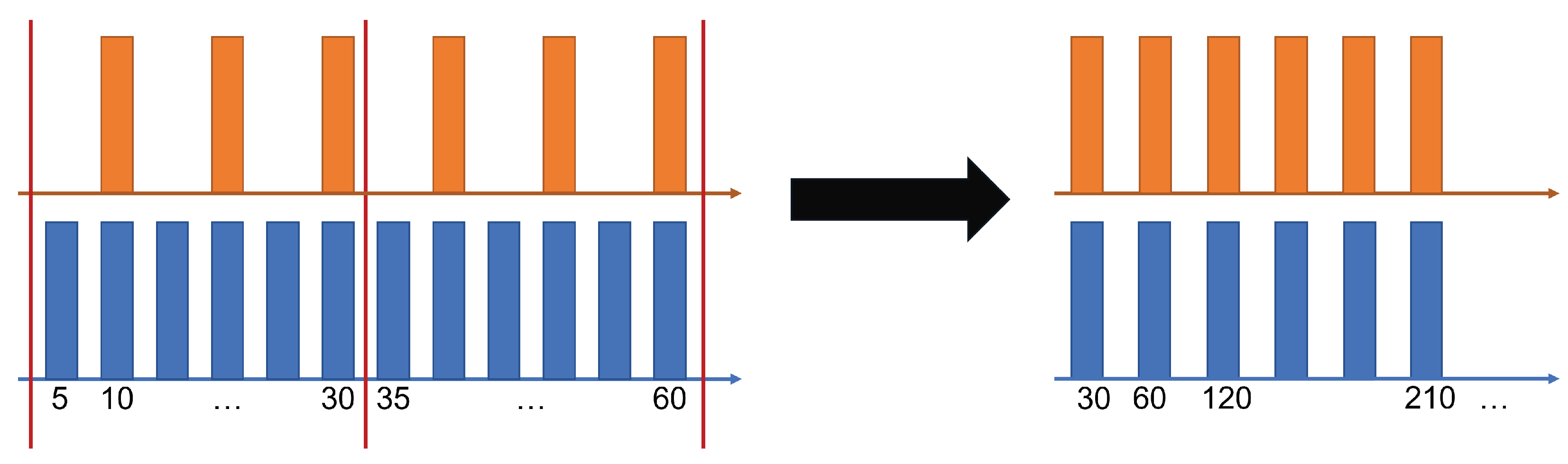
3.1.1. Different Frequencies

There are several ways to ensure that all data points have the same frequency (and in conclusion, the same timestamps). For example, one could only consider the data points that share the timestamp with at least one data point per other sensor. This brings the disadvantage of potentially discarding substantial amounts of data.

We therefore resampled all data points to one uniform sampling frequency of one data point every 30 min, also according to different rates at which the input sensors recorded their measurements. Depending on the sensor type (water level, discharge, and rainfall/precipitation), different resampling techniques were used. As the precipitation sensor measures the amount of rain fallen from the last measurement, we summed up all values inside a given 30 min interval. For the water level/discharge sensors, we utilized all values in a given 30 min interval, as here, the levels of height or intensity are recorded, not the amounts. Lastly, if all measurements inside an interval are missing, this results in a missing timestamp, which is handled by the data imputation. This is visualized in Figure 2.

3.1.2. Data Imputation

The battery-operated sensors offer flexibility regarding their placement along the Wupper, but they present a set of challenges regarding their power supply and data transfer reliability. These challenges include short outages due to the free, publicly usable network system that discards data packets when overloaded, and longer outages, such as those caused by depleted batteries. To ensure the usability of the sensor data, it was necessary to perform data imputation to fill in gaps in the time series.

We divided missing values into three types of gaps. A small gap is defined as a gap of less than 30 min, a middle gap is the interval between 30 min and 360 min, and a big gap is greater than 360 min. The 360 min threshold was selected based on the recommendations of hydrology experts, as data imputation techniques may not be effective for intervals of greater lengths. We filled the small gaps, inside the transformation to ensure consistent measuring intervals. The most common imputation techniques for time series involve either filling measurements with the mean or by linear interpolation ([46,47]).

As we transformed the interval by taking the mean of the measurements, filling missing data inside the interval with the mean would not affect the overall mean. Therefore, we were able to skip filling small gaps (<30 min) inside the data. For precipitation sensors, missing data inside the interval would affect the overall value, as those sum up all values. For those, we assumed nearly consistent rainfall through the overall interval and filled all missing values with the mean of the existing measurements.

Unlike smaller gaps, middle gaps in the water level and discharge sensor measurements cannot be ignored. Given that water cannot simply disappear but would need to change over time, our objective was to prevent a sudden decline in the water level by employing linear interpolation.

Such a linear relationship is not applicable to rain. While it might rain for the first measurement, it might instantly stop and be down to zero for the next one. We took the mean of the last value before and the first value after a gap, assuming a steady rainfall pattern. Luckily, precipitation sensors do not suffer from heavy gaps, and therefore do not need as much imputation, allowing this method to replace missing data.

3.1.3. Sensor Distances

We did not have direct access to the sensors, as they were provided by an external source, which limited our control over sensor deployment and maintenance. Additionally, detailed information on sensor calibration processes was unavailable, which may introduce some variability in measurement precision across stations. To support spatial context, we measured the distances between sensor stations, providing an intuitive reference frame for the spatial distribution of sensor locations (see

Table 1. Sensor–sensor distances: Distance in km measured between all sensors in the dataset. Sensors are either precipitation (Prec) or water level (WL) sensors. The main target sensor is “WL KLU”. Full sensor names can be taken from our published dataset.

	Prec BWV	Prec BUC	Prec HAR	Prec SCH	Prec WAL	Prec ZDD	Prec RO	Prec ROT	WL KLU	WL KRE
Prec BWV	0.0	8.11	3.02	1.78	10.25	3.53	5.44	5.45	3.4	9.88
Prec BUC		0.0	5.47	8.26	2.89	11.63	6.99	5.41	4.86	13.72
Prec HAR			0.0	2.79	7.31	6.41	5.82	4.99	0.67	11.77
Prec SCH				0.0	9.98	3.99	7.0	6.74	3.41	11.65
Prec WAL					0.0	13.72	9.86	8.29	6.85	16.6
Prec ZDD						0.0	7.89	8.42	6.88	9.96
Prec RO							0.0	1.58	5.43	6.76
Prec ROT								0.0	4.47	8.32
WL KLU									0.0	11.6
WL KRE										0.0

).

3.2. Methodology

To provide a quick overview on the performance of current state-of-the-art models on our dataset, we trained several models and compared their performance. This section briefly outlines the methods employed to train the models, as well as the steps taken to validate the results within the context of the given task. The objective of all models was to predict whether a given water level time series would exceed a critical threshold. This training method was used to train all of the models and was kept the same in order to ensure comparability.

All experiments were implemented in Python 3.9.19. The models were implemented with PyTorch (v2.2.2) [48], while the data preprocessing was performed with NumPy (v1.23.5) [49] and Pandas (v1.5.3) [50]. The evaluation was calculated using scikit-learn (v1.2.2) [51]. Due to the resource heavy calculation for some of the models, all experiments were run on an Ubuntu machine with an 96 x Intel Xeon Platinum 8186 CPU @ 2.7 GHz, 64 GB RAM and a single Nvidia Tesla V100 GPU.

3.2.1. Experimental Design

The approach to design the classification experiments was chosen as follows: The raw multi-channel (as multiple sensors were used) time-series data were cut into intervals of 96 h in length. From every interval, the first 48 h served as input for the neural networks tested in our approaches. The target to be predicted/classified was determined by evaluating whether the water level of the target sensor at Kluserbrücke exceeds a predetermined warning threshold of 125 cm in the next 6, 12, 24, or 48 h. Based on this, the target class would be either 0 (no warning) or 1 (warning) if the threshold is exceeded. With this method, every interval of 96 h could be given a label in regards to whether a warning should be issued or not. Nine state-of-the-art deep learning models (see

Table 2. Overview of selected time-series models.

Model	Reference	Architecture	Main Focus
DLinear	Zeng et al. [52]	Linear Layers	Efficient linear trend analysis for long-term time series
SegRNN	Lin et al. [30]	RNN	Long-term forecasting with segment-wise input iterations and parallel forecasting
TimesNet	Wu et al. [37]	CNN	Multiperiodicity modeling for enhanced feature representation in time series
Transformer	Vaswani et al. [32]	Transformer	Capturing temporal dependencies in general-purpose time-series data
PatchTST	Nie et al. [35]	Transformer	Patching mechanism for local feature extraction in temporal sequences
Informer	Zhou et al. [39]	Transformer	Sparse attention for scalable long-sequence forecasting
Non-stationary Transformer	Liu et al. [36]	Transformer	Adaptive handling of non-stationary series without stationarization
iTransformer	Liu et al. [38]	Transformer	Enhanced interpretability with focus on capturing long-range dependencies
Pyraformer	Liu et al. [45]	Transformer	Hierarchical pyramidal attention for efficient processing of long sequences

) were trained on this supervised learning task to predict a warning for a given time interval; their performance results were evaluated via accuracy, F1-score, precision, and recall. The selection of these models reflects a comprehensive representation of contemporary time-series architectures, encompassing various model structures. These include a model with linear layers, exemplified by DLinear; recurrent architectures such as SegRNN; convolutional neural network frameworks like TimesNet; and Transformer-based architectures including Transformer and PatchTST. Moreover, we incorporated models that leverage recent advancements in Transformer architectures, such as Informer, Non-stationary Transformer, Pyraformer, and iTransformer. Table 2 provides a detailed overview of these models, their architectures, and specific focus areas.

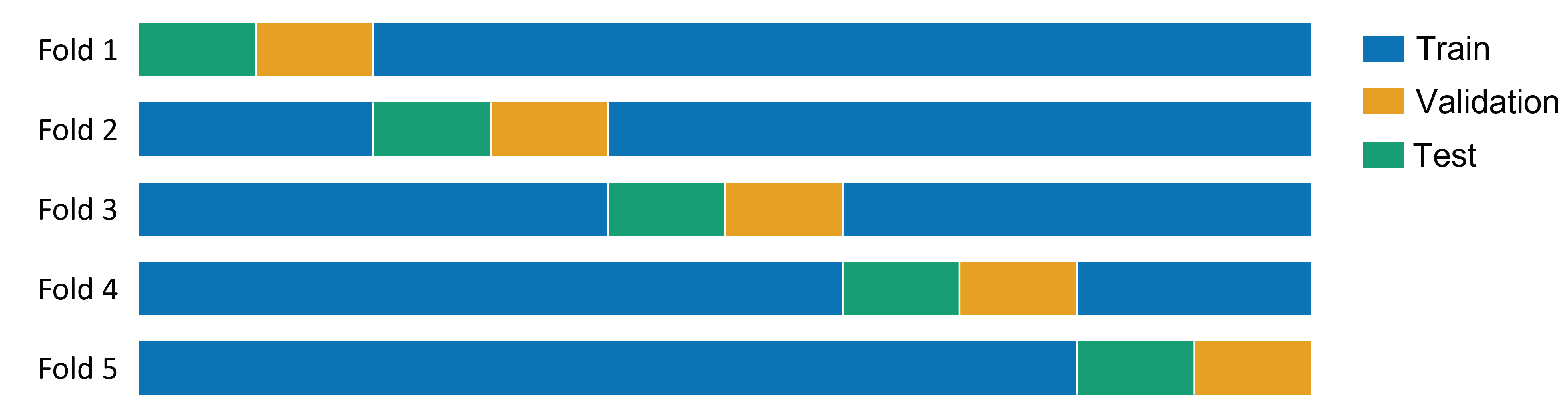
3.2.2. K-Fold Cross Validation

To ensure reliable results, we employed a variant, adapted to the use case, of the k-fold cross-validation [53] procedure, with k equal to five. Due to the imbalanced nature of the dataset between the two classes, an algorithm was implemented to split the data into three distinct sets: a training set, a validation set, and a test set. The data were initially split into two sets, one comprising instances of flood events and the other comprising instances of non-flood events. Both sets were then shuffled. The initial 10% of each of the two lists was designated as test data, with the subsequent 10% serving as the validation data. The remaining data were automatically designated as training data. This process was repeated five times, with the test and validation data windows being shifted by 20% of the data each time. Figure 3 visualizes how the test, validation, and train data were selected for each fold.

3.2.3. Hyperparameter Search

The initial step involved conducting a hyperparameter search using the Python package Optuna. A total of 50 trials were conducted for each model. Each of those trials consisted of the following:

• We performed a random search ([54]) on hyperparameters, such as learning rate, training epochs, and model-specific parameters.
• Training the model on a reduced subset of train data from the first fold.
• Evaluating the models’ performance (in regards to the F1-score), using the validation dataset from the first fold.

For each model, we saved the hyperparameters that produced the highest F1-score for future use.

3.2.4. Training

Using the hyperparameters found in the previous step, we trained each chosen model on the training data of the first fold. The model would have been trained for a maximum of 50 epochs, but training involved an early stopping mechanism with a patience threshold of 7.

4. Experiments

4.1. Flood Warning Event Forecasting

The flood warning classification experiments, using nine different tested model architectures, resulted in different outcomes regarding the models’ capabilities to correctly issue warnings, shown in

Table 3. The classification results of flood warning. Bold values indicate the best scores.

Model	Accuracytest	F1-Scoretest	Precisiontest	Recalltest
Transformer	0.762 ± 0.241	0.212 ± 0.101	0.131 ± 0.071	0.902 ± 0.140
Pyraformer	0.981 ± 0.005	0.630 ± 0.060	0.476 ± 0.071	0.954 ± 0.021
DLinear	0.987 ± 0.001	0.709 ± 0.020	0.567 ± 0.025	0.946 ± 0.015
iTransformer	0.993 ± 0.001	0.819 ± 0.021	0.736 ± 0.025	0.923 ± 0.022
PatchTST	0.994 ± 0.001	0.831 ± 0.020	0.762 ± 0.031	0.914 ± 0.025
Informer	0.995 ± 0.001	0.867 ± 0.013	0.809 ± 0.022	0.936 ± 0.018
Non-stationary Transformer	0.996 ± 0.000	0.889 ± 0.011	0.857 ± 0.023	0.926 ± 0.021
TimesNet	0.997 ± 0.001	0.896 ± 0.014	0.876 ± 0.033	0.918 ± 0.017
SegRNN	0.997 ± 0.000	0.910 ± 0.011	0.906 ± 0.021	0.914 ± 0.019

. All models, besides Transformer, achieved accuracies higher than 98%. Comparably, each model achieved recall values greater than 90%, indicating that more than 90% of real warning cases were caught by the models and less than 10% of warning-worthy events were missed. Here, the Transformer architecture demonstrates higher variability in recall compared to other models, by showing a standard deviation of 14%, making the result less reliable for this model. Precision values exhibit considerable variation across different models. The lowest precision is observed in the transformer model, at approximately 13%. In contrast, the majority of models demonstrate precision levels ranging from 45% to 80%. Notably, the highest precision is achieved by the Non-stationary Transformer, TimesNet, and SegRNN models, with values approaching or exceeding 90%. Qualitatively, precision indicates the relative amount warnings that were correct, e.g., warnings where a warning was justified. Results of the F1-score show the same relative behavior as the precision values. While the Pyraformer demonstrates the strongest performance in recall among the models, it shows the second-worst precision score, as well as a lower F1-score. The SegRNN architecture demonstrates the highest performance in our study, exhibiting an F1-score that is notably superior to those of Pyraformer and DLinear, which exhibit higher recall values.

4.2. Case Study Extreme Events

After evaluating the deep learning algorithms, the best performing model SegRNN was chosen for further elaboration. A select few exemplary time-series intervals were chosen and depicted to illustrate cases of successful and unsuccessful classification.

The first two curves in Figure 4a,b illustrate the classical and intuitive flooding phenomena, wherein precipitation events result in progressively elevated water levels until the warning threshold is surpassed. Example Figure 4c demonstrates a high-intensity, short-term rainfall event with a stronger and sharper rise in water levels. The last curve Figure 4d shows the occurrence of a very common example for a successful warning classification, where the water level in the input time frame already exceeds the warning threshold, and no greater, dynamic changes in the water level occur.

Figure 5 shows two examples where the model was not able to issue a warning-worthy prediction but a warning would still have been justified and necessary. Figure 5a shows a very intense short-term rain event leading to a sudden spike in water levels. This is one potential explanation for the misclassification of the interval, given that the dynamic of the situation unfolded more rapidly than could be captured in our dataset, which only included a single data point every 30 min. Possibly due to only few available data in general showing this specific rainfall behavior, training the model to react accordingly could prove difficult. The second negative example Figure 5b shows a misclassification as well, where the water level was, in a stable way, oscillating around the warning threshold of 125 cm.

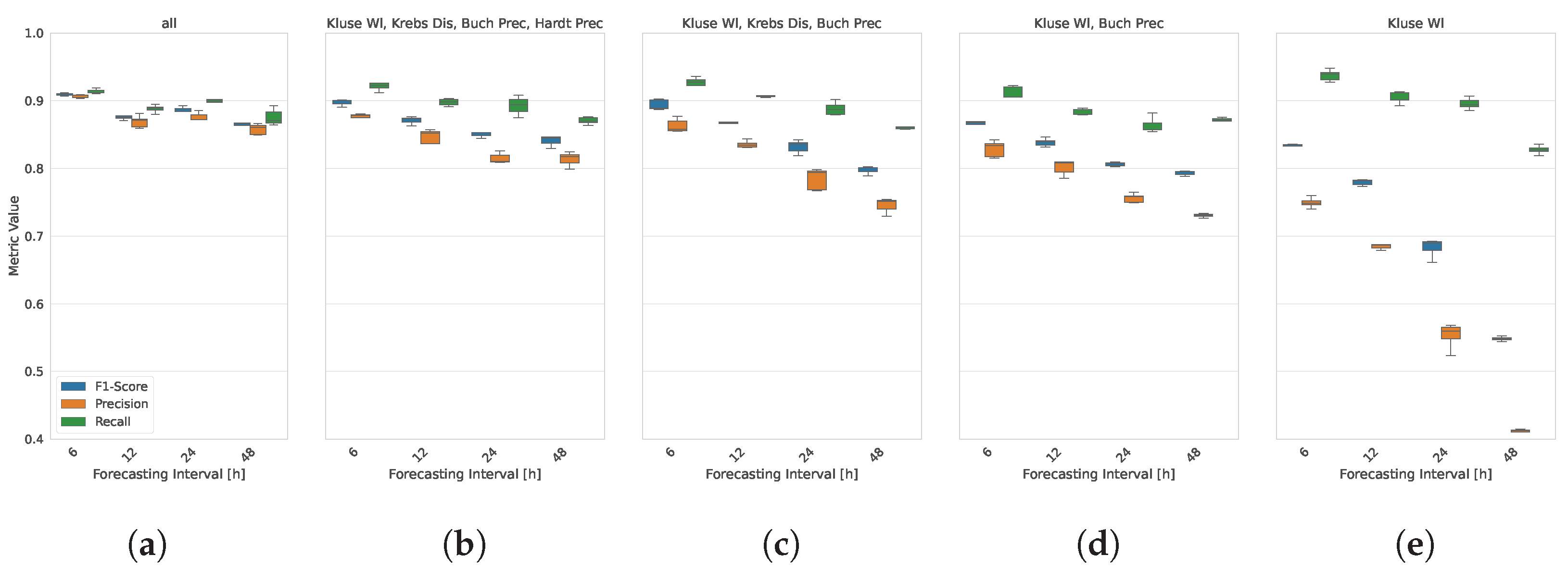
4.3. Minimum Viable Sensor Count

The objective of the following experiments was to investigate the impact of a reduced sensor count on the efficacy of a flood prediction model in issuing accurate flood warnings. A reduced sensor count that still provides sufficient data for a model to make reliable predictions would allow for smaller and more cost-effective sensor installations and demonstrated viability of a model, even if sensors are temporarily unavailable (e.g., due to a defect). Additionally, the effect on the prediction/warning quality of prolonging the future time intervals of 6 h, 12 h, 24 h, or 48 h in which a possible flood event could occur was evaluated. Figure 6 displays the baseline performance on the left with all sensors available, feeding input into our trained model. Over longer prediction time intervals, the baseline model shows slight declines of ~3–5% for precision and recall. The second part of the figure, showing a model only influenced by the input of one upriver discharge sensor and two precipitation sensors, demonstrates a stronger initial difference between recall and precision. As the forecasting interval lengthens, the discrepancy between recall and precision widens. While recall remains relatively consistent, precision declines to approximately 75%.

As the number of sensors is reduced, the relative behavior is maintained. This is demonstrated in Figure 6c,d, where the removal of a precipitation sensor in Figure 6c and an upriver discharge sensor in Figure 6d both result in a reduction in precision when compared to Figure 6b. The strongest decline in performance shows the last part of the figure, showcasing a model that tries to predict flood events by only looking at the past water levels and no further sensor inputs. For the shortest forecasting interval, the precision lies around 75% and drops over increasing intervals to ultimately reach approximately 40%. The overall trend is a reduction in precision when the sensor count is reduced and the forecasting intervals are increasing. Interestingly, the recall for all model conditions remains stable and similar in a range of around 90% (lowest 82%, highest 94%).

5. Conclusions

Our study makes significant contributions to flood forecasting research by applying deep learning models to a comprehensive multi-sensor dataset from the Wupper River region. Through an extensive evaluation of various state-of-the-art models, we demonstrate that deep learning approaches can effectively issue timely and accurate flood warnings with high reliability. The primary contributions of this work are as follows:

• We present a unique, publicly available dataset comprising several years of data from three types of sensors—water level, discharge, and precipitation—strategically positioned throughout Wuppertal and its surrounding areas. This dataset serves as a valuable resource for flood forecasting research and model benchmarking.
• We evaluate the performance of multiple deep learning models, demonstrating their ability to issue reliable flood warnings with high accuracy. Our top-performing algorithm, the SegRNN model, successfully issued warnings in approximately 91% of flood occurrences, underscoring the effectiveness of deep learning for flood forecasting.
• Our results indicate a false warning rate of approximately 10%, highlighting the importance of balancing sensitivity and specificity in flood prediction applications. This finding offers valuable insights into model performance trade-offs and suggests potential areas for enhancing flood warning accuracy.

These results demonstrate the general usability of this approach to warn local communities ahead of time of the danger of a flood event in the next six hours. Whether the yielded results are reliable enough has to be debated though. This very much depends on the nature of the 9% missed flood events and the consequences of false warnings for the people threatened by flood events.

In the event that the 9% of unanticipated occurrences predominantly encompass instances where a flood has already occurred and the water levels are merely sufficient to trigger a sequence of continuous alerts, and a few of these alerts are misidentified, the consequences for the individuals affected are likely to be minimal. If, on the other hand, these missed events are for example highly spontaneous, short-termed but intense flood events, then people and property could pay a hefty cost for these 9% of missed events. A thorough analysis of the missed flooding events is paramount to understand the nature of the model’s incompetence to capture these cases and to judge its severity.

In case of false warnings, the case is even more complicated. If the consequences of a warning are dire, like the seizing of local production, installations of flood defense mechanisms, or evacuation procedures, then every false warning can be very costly for a community and local companies. Additionally, false warnings can lead to desensitization towards warnings in people if they learn that warnings are unreliable and in the worst case can prevent people from showing the proper life- and property-saving behavior in case a warning is issued that is followed by a real flood event. In terms of a reduced sensor count, the results show a clear connection between the quality of the prediction and the number of sensors and/or the prediction interval’s length.

The general tendency can be described as a decrease in precision as the sensor number is reduced and the prediction interval length is increased. Nevertheless, the first sensor-reduced test using only two precipitation sensors, one discharge sensors, and the target sensor itself, so an overall of four sensors only, does not show drastically reduced performance compared to the experiment using all sensors. The precision decrease is only about 2–8%, depending on prediction interval length. Lower sensor numbers reduce precision further, but it still remains over $80\%$ using only one precipitation sensor and the target water level if predicted six hours into the future.

The results demonstrate the applicability of even small sensor arrangements to capture useful information and issue warnings that are reliable to a measurable degree. Even given limited resources, this sensor-driven approach could prove useful in different regions by installing a small number of precipitation sensors and one or several water level measurement stations, where predictions or warnings are to be issued.

The dataset that is provided in our work may serve as benchmark for similar endeavors as in predicting warnings for flood events or directly predicting water levels several hours into the future. The dataset itself holds more than a decade worth of high-quality sensor data and was proven to train several different machine learning architectures in useful flood warning solutions.

Outlook

Training deep learning algorithms to generate flood warnings is definitely useful but in no way the end, toward which this dataset or the general approach towards AI-based flood prediction can and should be driven. A next logical step would be to elevate the task from simple classification into a regression task, where the next several hours of the water level at a certain position are predicted. This continuous prediction, in the best case created with a measure for its uncertainty, would allow for a better understanding of the water level development in the next hours than a simple classification. Depending on the location and available resources, actions like temporary dams or evacuations could be instated to save property and lives more precisely in a measured response.

Missing data points in continuous time-series data are a common problem and were addressed by either discarding incomplete data intervals or by leveraging simple imputation techniques. There are, however, more elaborate ways to deal with missing data, for example, soft sensor techniques that use a machine learning approach to generate missing sensor data based on still available sensor channels.

Furthermore, to address the challenge of reducing the $9\%$ of flood events that currently go unpredicted, it is essential to incorporate more of these rare events into the training datasets for deep learning models. As such events are characteristically scarce, an effective method for augmenting the training data could entail the synthetic generation of these events or the utilization of high-fidelity simulations to generate representative scenarios. By enriching the dataset with these additional examples, the models could be better equipped to identify and predict these critical yet infrequent events, thereby improving the overall prediction accuracy and reliability.

Overall, the usage of small local sensor ensembles in combination with machine learning-based solutions for local flood warning issuing seems very promising and fruitful to explore further.

References

1. Myhre, G.; Alterskjær, K.; Stjern, C.W.; Hodnebrog, Ø.; Marelle, L.; Samset, B.H.; Sillmann, J.; Schaller, N.; Fischer, E.; Schulz, M.; et al. Frequency of extreme precipitation increases extensively with event rareness under global warming. Sci. Rep. 2019, 9, 16063. [Google Scholar] [CrossRef] [PubMed]
2. Unisdr, C. The Human Cost of Natural Disasters: A Global Perspective. 2015. Available online: https://climate-adapt.eea.europa.eu/en/metadata/publications/the-human-cost-of-natural-disasters-2015-a-global-perspective (accessed on 20 November 2024).
3. Biswas, A.K. History of Hydrology; North-Holland Publishing: Amsterdam, The Netherlands, 1970. [Google Scholar]
4. Hakim, D.K.; Gernowo, R.; Nirwansyah, A.W. Flood prediction with time series data mining: Systematic review. Nat. Hazards Res. 2024, 4, 194–220. [Google Scholar] [CrossRef]
5. Ahmed, M.I.; Stadnyk, T.; Pietroniro, A.; Awoye, H.; Bajracharya, A.; Mai, J.; Tolson, B.A.; Shen, H.; Craig, J.R.; Gervais, M.; et al. Learning from hydrological models’ challenges: A case study from the Nelson basin model intercomparison project. J. Hydrol. 2023, 623, 129820. [Google Scholar] [CrossRef]
6. Souffront Alcantara, M.A.; Nelson, E.J.; Shakya, K.; Edwards, C.; Roberts, W.; Krewson, C.; Ames, D.P.; Jones, N.L.; Gutierrez, A. Hydrologic Modeling as a Service (HMaaS): A New Approach to Address Hydroinformatic Challenges in Developing Countries. Front. Environ. Sci. 2019, 7, 158. [Google Scholar] [CrossRef]
7. Kumar, V.; Azamathulla, H.M.; Sharma, K.V.; Mehta, D.J.; Maharaj, K.T. The State of the Art in Deep Learning Applications, Challenges, and Future Prospects: A Comprehensive Review of Flood Forecasting and Management. Sustainability 2023, 15, 10543. [Google Scholar] [CrossRef]
8. Bentivoglio, R.; Isufi, E.; Jonkman, S.N.; Taormina, R. Deep learning methods for flood mapping: A review of existing applications and future research directions. Hydrol. Earth Syst. Sci. 2022, 26, 4345–4378. [Google Scholar] [CrossRef]
9. Wönkhaus, M.; Hahn, Y.; Kienitz, P.; Meyes, R.; Meisen, T. Flood Classification Dataset from the River Wupper in Germany. Zenodo 2024. [Google Scholar] [CrossRef]
10. Jain, S.K.; Mani, P.; Jain, S.K.; Prakash, P.; Singh, V.P.; Tullos, D.; Kumar, S.; Agarwal, S.P.; Dimri, A.P. A Brief review of flood forecasting techniques and their applications. Int. J. River Basin Manag. 2018, 16, 329–344. [Google Scholar] [CrossRef]
11. Kauffeldt, A.; Wetterhall, F.; Pappenberger, F.; Salamon, P.; Thielen, J. Technical review of large-scale hydrological models for implementation in operational flood forecasting schemes on continental level. Environ. Model. Softw. 2016, 75, 68–76. [Google Scholar] [CrossRef]
12. Jehanzaib, M.; Ajmal, M.; Achite, M.; Kim, T.W. Comprehensive Review: Advancements in Rainfall-Runoff Modelling for Flood Mitigation. Climate 2022, 10, 147. [Google Scholar] [CrossRef]
13. Lindström, G.; Johansson, B.; Persson, M.; Gardelin, M.; Bergström, S. Development and test of the distributed HBV-96 hydrological model. J. Hydrol. 1997, 201, 272–288. [Google Scholar] [CrossRef]
14. Cronshey, R. Urban Hydrology for Small Watersheds; Number 55; US Department of Agriculture, Soil Conservation Service, Engineering Division: Washington, DC, USA, 1986. [Google Scholar]
15. Arnold, J.G.; Srinivasan, R.; Muttiah, R.S.; Williams, J.R. Large Area Hydrologic Modeling and Assessment Part I: Model Development. JAWRA J. Am. Water Resour. Assoc. 1998, 34, 73–89. [Google Scholar] [CrossRef]
16. Norbiato, D.; Borga, M.; Dinale, R. Flash flood warning in ungauged basins by use of the flash flood guidance and model-based runoff thresholds. Meteorol. Appl. 2009, 16, 65–75. [Google Scholar] [CrossRef]
17. Cannon, S.H.; Gartner, J.E.; Wilson, R.C.; Bowers, J.C.; Laber, J.L. Storm rainfall conditions for floods and debris flows from recently burned areas in southwestern Colorado and southern California. Geomorphology 2008, 96, 250–269. [Google Scholar] [CrossRef]
18. Hapuarachchi, H.A.P.; Wang, Q.J.; Pagano, T.C. A review of advances in flash flood forecasting. Hydrol. Processes 2011, 25, 2771–2784. [Google Scholar] [CrossRef]
19. Giannaros, C.; Dafis, S.; Stefanidis, S.; Giannaros, T.M.; Koletsis, I.; Oikonomou, C. Hydrometeorological analysis of a flash flood event in an ungauged Mediterranean watershed under an operational forecasting and monitoring context. Meteorol. Appl. 2022, 29, e2079. [Google Scholar] [CrossRef]
20. Zhao, X.; Wang, H.; Bai, M.; Xu, Y.; Dong, S.; Rao, H.; Ming, W. A Comprehensive Review of Methods for Hydrological Forecasting Based on Deep Learning. Water 2024, 16, 1407. [Google Scholar] [CrossRef]
21. Gude, V.; Corns, S.; Long, S. Flood Prediction and Uncertainty Estimation Using Deep Learning. Water 2020, 12, 884. [Google Scholar] [CrossRef]
22. Luppichini, M.; Barsanti, M.; Giannecchini, R.; Bini, M. Deep learning models to predict flood events in fast-flowing watersheds. Sci. Total Environ. 2022, 813, 151885. [Google Scholar] [CrossRef]
23. Widiasari, I.R.; Nugroho, L.E.; Widyawan. Deep learning multilayer perceptron (MLP) for flood prediction model using wireless sensor network based hydrology time series data mining. In Proceedings of the 2017 International Conference on Innovative and Creative Information Technology (ICITech), Salatiga, Indonesia, 2–4 November 2017; IEEE: Piscataway, NJ, USA, 2017; pp. 1–5. [Google Scholar] [CrossRef]
24. Chen, C.; Jiang, J.; Liao, Z.; Zhou, Y.; Wang, H.; Pei, Q. A short-term flood prediction based on spatial deep learning network: A case study for Xi County, China. J. Hydrol. 2022, 607, 127535. [Google Scholar] [CrossRef]
25. Wu, Z.; Zhou, Y.; Wang, H.; Jiang, Z. Depth prediction of urban flood under different rainfall return periods based on deep learning and data warehouse. Sci. Total Environ. 2020, 716, 137077. [Google Scholar] [CrossRef] [PubMed]
26. Kimura, N.; Yoshinaga, I.; Sekijima, K.; Azechi, I.; Baba, D. Convolutional Neural Network Coupled with a Transfer-Learning Approach for Time-Series Flood Predictions. Water 2019, 12, 96. [Google Scholar] [CrossRef]
27. Sankaranarayanan, S.; Prabhakar, M.; Satish, S.; Jain, P.; Ramprasad, A.; Krishnan, A. Flood prediction based on weather parameters using deep learning. J. Water Clim. Chang. 2020, 11, 1766–1783. [Google Scholar] [CrossRef]
28. Zhao, G.; Liu, R.; Yang, M.; Tu, T.; Ma, M.; Hong, Y.; Wang, X. Large-scale flash flood warning in China using deep learning. J. Hydrol. 2022, 604, 127222. [Google Scholar] [CrossRef]
29. Panahi, M.; Jaafari, A.; Shirzadi, A.; Shahabi, H.; Rahmati, O.; Omidvar, E.; Lee, S.; Bui, D.T. Deep learning neural networks for spatially explicit prediction of flash flood probability. Geosci. Front. 2021, 12, 101076. [Google Scholar] [CrossRef]
30. Lin, S.; Lin, W.; Wu, W.; Zhao, F.; Mo, R.; Zhang, H. SegRNN: Segment Recurrent Neural Network for Long-Term Time Series Forecasting. arXiv 2023, arXiv:2308.11200. [Google Scholar]
31. Chung, J.; Gulcehre, C.; Cho, K.; Bengio, Y. Empirical Evaluation of Gated Recurrent Neural Networks on Sequence Modeling. arXiv 2014, arXiv:1412.3555. [Google Scholar]
32. Vaswani, A.; Shazeer, N.; Parmar, N.; Uszkoreit, J.; Jones, L.; Gomez, A.N.; Kaiser, Ł.; Polosukhin, I. Attention is all you need. In Proceedings of the 31st Conference on Neural Information Processing Systems (NIPS 2017), Long Beach, CA, USA, 4–9 December 2017; Volume 30. [Google Scholar]
33. Wen, Q.; Zhou, T.; Zhang, C.; Chen, W.; Ma, Z.; Yan, J.; Sun, L. Transformers in Time Series: A Survey. arXiv 2023, arXiv:2202.07125. [Google Scholar]
34. Lim, B.; Arık, S.O.; Loeff, N.; Pfister, T. Temporal Fusion Transformers for interpretable multi-horizon time series forecasting. Int. J. Forecast. 2021, 37, 1748–1764. [Google Scholar] [CrossRef]
35. Nie, Y.; Nguyen, N.H.; Sinthong, P.; Kalagnanam, J. A Time Series is Worth 64 Words: Long-term Forecasting with Transformers. arXiv 2023, arXiv:2211.14730. [Google Scholar]
36. Liu, Y.; Wu, H.; Wang, J.; Long, M. Non-stationary Transformers: Exploring the Stationarity in Time Series Forecasting. arXiv 2022, arXiv:2205.14415. [Google Scholar] [CrossRef]
37. Wu, H.; Hu, T.; Liu, Y.; Zhou, H.; Wang, J.; Long, M. Timesnet: Temporal 2d-variation modeling for general time series analysis. In Proceedings of the Eleventh International Conference on Learning Representations, Virtual Event, 25–29 April 2022. [Google Scholar]
38. Liu, Y.; Hu, T.; Zhang, H.; Wu, H.; Wang, S.; Ma, L.; Long, M. iTransformer: Inverted Transformers Are Effective for Time Series Forecasting. arXiv 2024, arXiv:2310.06625. [Google Scholar] [CrossRef]
39. Zhou, H.; Zhang, S.; Peng, J.; Zhang, S.; Li, J.; Xiong, H.; Zhang, W. Informer: Beyond Efficient Transformer for Long Sequence Time-Series Forecasting. Proc. AAAI Conf. Artif. Intell. 2021, 35, 11106–11115. [Google Scholar] [CrossRef]
40. Zhang, G.P. Time series forecasting using a hybrid ARIMA and neural network model. Neurocomputing 2003, 50, 159–175. [Google Scholar] [CrossRef]
41. Bandara, K.; Bergmeir, C.; Smyl, S. Forecasting across time series databases using recurrent neural networks on groups of similar series: A clustering approach. Expert Syst. Appl. 2020, 140, 112896. [Google Scholar] [CrossRef]
42. Wen, Q.; Yang, F.; Song, X.; Gao, Y.; Zhao, P.; Deng, H. A robust decomposition approach to forecasting in the presence of anomalies: A case study on web traffic. IEEE Trans. Knowl. Data Eng. 2020, 32, 2398–2409. [Google Scholar]
43. Cleveland, R.B.; Cleveland, W.S.; McRae, J.E.; Terpenning, I. STL: A seasonal-trend decomposition procedure based on loess. J. Off. Stat. 1990, 6, 3–73. [Google Scholar]
44. Zhou, T.; Ma, Z.; Wen, Q.; Wang, X.; Sun, L.; Jin, R. FEDformer: Frequency Enhanced Decomposed Transformer for Long-term Series Forecasting. In Proceedings of the 39th International Conference on Machine Learning, Proceedings of Machine Learning Research, Baltimore, MD, USA, 17–23 July 2022; Chaudhuri, K., Jegelka, S., Song, L., Szepesvari, C., Niu, G., Sabato, S., Eds.; PMLR 162. pp. 27268–27286. [Google Scholar]
45. Liu, S.; Yu, H.; Liao, C.; Li, J.; Lin, W.; Liu, A.X.; Dustdar, S. Pyraformer: Low-Complexity Pyramidal Attention for Long-Range Time Series Modeling and Forecasting. In Proceedings of the International Conference on Learning Representations, Virtual, 25 April 2022. [Google Scholar]
46. Noor, N.M.; Al Bakri Abdullah, M.M.; Yahaya, A.S.; Ramli, N.A. Comparison of Linear Interpolation Method and Mean Method to Replace the Missing Values in Environmental Data Set. Mater. Sci. Forum 2014, 803, 278–281. [Google Scholar] [CrossRef]
47. Wolbers, M.; Noci, A.; Delmar, P.; Gower-Page, C.; Yiu, S.; Bartlett, J.W. Standard and reference-based conditional mean imputation. Pharm. Stat. 2022, 21, 1246–1257. [Google Scholar] [CrossRef]
48. Paszke, A.; Gross, S.; Massa, F.; Lerer, A.; Bradbury, J.; Chanan, G.; Killeen, T.; Lin, Z.; Gimelshein, N.; Antiga, L.; et al. PyTorch: An imperative style, high-performance deep learning library. In Proceedings of the 33rd International Conference on Neural Information Processing Systems, Vancouver, BC, Canada, 8–14 December 2019; Curran Associates Inc.: Red Hook, NY, USA, 2019. [Google Scholar]
49. Harris, C.R.; Millman, K.J.; van der Walt, S.J.; Gommers, R.; Virtanen, P.; Cournapeau, D.; Wieser, E.; Taylor, J.; Berg, S.; Smith, N.J.; et al. Array programming with NumPy. Nature 2020, 585, 357–362. [Google Scholar] [CrossRef]
50. Reback, J.; McKinney, W.; Jbrockmendel; Van den Bossche, J.; Augspurger, T.; Cloud, P.; Hawkins, S.; Gfyoung; Sinhrks; Petersen, T.; et al. pandas-dev/pandas: Pandas; Zenodo: Geneva, Switzerland, 2020. [Google Scholar] [CrossRef]
51. Pedregosa, F.; Varoquaux, G.; Gramfort, A.; Michel, V.; Thirion, B.; Grisel, O.; Blondel, M.; Prettenhofer, P.; Weiss, R.; Dubourg, V.; et al. Scikit-learn: Machine learning in Python. J. Mach. Learn. Res. 2011, 12, 2825–2830. [Google Scholar]
52. Zeng, A.; Chen, M.; Zhang, L.; Xu, Q. Are transformers effective for time series forecasting? In Proceedings of the AAAI Conference on Artificial Intelligence, Washington, DC, USA, 7–14 February 2023; Volume 37, pp. 11121–11128. [Google Scholar] [CrossRef]
53. Arlot, S.; Celisse, A. A survey of cross-validation procedures for model selection. Stat. Surv. 2010, 4. [Google Scholar] [CrossRef]
54. Bergstra, J.; Bengio, Y. Random search for hyper-parameter optimization. J. Mach. Learn. Res. 2012, 13, 281–305. [Google Scholar]
Figure 1. The placement of the discharge sensor at the Wuppertalsperre (marked 1), the discharge and water level sensor at Kluserbrücke (marked 2), and the river Wupper, highlighted in blue.
Water 16 03368 g001
Figure 2. Depiction of the used resampling strategy where sensor measurements are recorded with varying frequencies (e.g., one data point every five or ten minutes). All data were resampled to one value every 30 min.
Water 16 03368 g002
Figure 3. Visualization of the data split across training, validation, and test sets for each fold.
Water 16 03368 g003
Figure 4. Four examples of special flood warning events where water levels at the target sensor exceeded the 125 cm warning threshold (red dashed line), correctly predicted by the deep learning classifier. The orange line shows water levels during the input interval, the green line represents levels during the warning interval to be classified, and rainfall intensity is depicted by light-blue bars. (a) Positive classification example. (b) Positive classification example. (c) Positive classification example—heavy summer rain. (d) Common positive classification example—constant rain.
Water 16 03368 g004
Figure 5. Special flood warning events. This representation shows 2 exemplary events, where the target sensor’s water level did exceed the warning threshold of 125 cm (red dashed line), but a warning was not issued by the machine learning classifier. These intervals were misclassified. (a) High-intensity, short-term rainfall event—misclassification example. (b) Water level close to the warning threshold—misclassification event.
Water 16 03368 g005
Figure 6. Comparison of different sensor combinations and label time intervals.
Water 16 03368 g006