Study on the Spatiotemporal Evolution Pattern of Frazil Ice Based on CFD-DEM Coupled Method

Abstract

Frazil ice is the foundation for all other ice phenomena, and its spatiotemporal evolution is critical for regulating ice conditions in rivers and channels, as well as for preventing and controlling ice damage. This paper investigates the dynamic transport pattern of frazil ice during the early stages of winter freezing in water conveyance channels based on a CFD-DEM coupled numerical model, and derives predictive formulae for the spatiotemporal evolution of frazil ice and floating ice. First, static repose angle simulations and slope sliding simulations were used to calibrate the contact parameters between frazil ice particles and between frazil ice and the channel bed, ensuring the accurate calculation of contact forces in the model. On this basis, the processes of frazil ice transport, aggregation, and upward movement in water transfer channels were simulated, and the influence of contact parameters on simulation results was analyzed, showing a significant effect when the ice concentration was high. Numerical results indicate that the amount of suspended frazil ice is positively correlated with the frazil ice generation rate and water depth, with minimal influence from the flow velocity; the amount of floating ice increases linearly along the channel, with growth positively correlated with the frazil ice generation rate and water depth, and negatively correlated with the flow velocity. Predictive formulae correlating frazil ice and floating ice amounts with the flow velocity, water depth, and other factors were proposed based on numerical results. There is good agreement between the predictive and numerical results: the maximum APE between the predicted and simulated values of suspended frazil ice is 13.24%, and the MAPE is 6.32%; the maximum APE between the predicted and simulated values of floating ice increment is 7.80%, and the MAPE is 2.89%. The proposed prediction formulae can provide a theoretical basis for accurately predicting ice conditions during the early stages of winter freezing in rivers and channels.

1. Introduction

The Middle Route of the South-to-North Water Transfer Project begins at the Danjiangkou Reservoir in Hubei Province, passes through Henan and Hebei provinces, and reaches Beijing and Tianjin, crossing multiple climatic zones, including subtropical monsoon and temperate continental monsoon climates. During winter, temperatures in regions north of the Yellow River remain below 0 °C for extended periods, leading to heat loss in water conveyance channels and causing various ice conditions, such as shore ice, drifting ice, and ice cover, with freezing periods lasting from one to three months. Simultaneously, the channels encounter various forms of ice-related issues [1], such as damage to hydraulic structures caused by upstream ice impacts, the formation of ice jams that elevate upstream water levels, potentially leading to ice-induced floods and disruptions to navigation [2], and the scouring of certain channel sections by ice, which can compromise the habitats of fish and other wildlife populations [3]. These ice-related issues stem from the formation and evolution of frazil ice. As the fundamental ice form in river and channel ice issues, the dynamic transport process of frazil ice influences the subsequent development and evolution of the ice condition. Particularly during the early stages of winter freezing, the dynamic behavior of frazil ice is critical to the formation and distribution of floating ice. Failure to regulate channel operation conditions in a timely manner can lead to ice storms. To ensure the operational safety of the channel, the Middle Route of the South-to-North Water Transfer Project currently operates primarily with an under-ice cover transfer mode. However, due to the lack of efficient and accurate ice prediction, the timing of switching water transfer modes during the current ice period often relies on historical empirical judgements, making it difficult to accurately regulate the scope and duration of water transfer modes under the ice cover, which can easily lead to a decline in water transfer efficiency and an increase in the risk of ice-breaking disasters. Therefore, in-depth research on the transport and evolution patterns of frazil ice has significant scientific value in improving the timeliness of ice predicting for water transfer projects.

Most studies on the evolution of frazil ice have been conducted under laboratory conditions, with the earliest dating back to 1950, when Schaefer [4] conducted experiments on the formation and evolution of frazil ice in an outdoor flume. Subsequently, Hanley and Michel et al. [5,6] studied the phenomenon of water supercooling and freezing under different temperature and water flow conditions using cylindrical steel tanks in the freezer compartment. The water flow rate was controlled by a variable speed propeller. Clark et al. [7,8] designed a counter-rotating water tank and adjusted the turbulence intensity by changing the roughness of the rotating bottom plate and side walls, effectively avoiding the influence of the experimental facility on the formation and evolution of frazil ice. Laboratory experiments on the formation and evolution of frazil ice are limited by the hydraulic and thermal conditions, and technical and spatial scales, making it difficult to accurately simulate the dynamic transport process of frazil ice, and the extraction of relevant data also faces challenges [9].

Compared with experimental studies, field observations can obtain more accurate data on the formation and evolution of frazil ice. Ghobrial et al. [10] used high-frequency and low-frequency sonar to detect frazil ice, combined with a scattering model to estimate the concentration and size of frazil ice. The disc model was found to be the most suitable when compared with the experimental data. With the development of digital image technology, researchers have observed the shape and quantity of frazil ice more accurately. McFarlane et al. [11,12] designed a new underwater imaging system that enabled the first quantitative measurement of frazil ice’s shape and size distribution as it evolves in a natural river. The results were in general agreement with the experimental data. Many scholars [13,14,15,16,17] have also proposed theoretical formulae for calculating the floating speed of frazil ice based on field observations and experimental data. However, these formulae do not take into account the angle of frazil ice floating and the effects of turbulence. Although experimental studies and field observations are effective methods, they are costly and it is difficult to carry out a large number systematic studies on the spatiotemporal evolution of ice conditions.

The rapid development of computer technology has led to the gradual rise of numerical simulation technology in the field of ice hydraulics. Researchers have carried out many studies focusing on the nucleation, growth, and flocculation processes of frazil ice. Hammar et al. [18] established a model for the formation and evolution of frazil ice in open channels based on the heat transfer rate between water columns, which can simulate variations in frazil ice size, concentration, and water temperature. Wang et al. [19] improved the nucleation, growth, and floc breakup processes of frazil ice using a variable Nusselt number related to turbulence, and developed a new mathematical model that can simulate the supercooling process and the evolution of frazil ice. Other scholars have also developed various mathematical models for frazil ice based on similar theories of crystal nucleation, secondary nucleation, and flocculation [14,20,21,22]. Additionally, some researchers have explored frazil ice movement and distribution patterns using mathematical models. Liou et al. [23] linked the impact of turbulence to the rising motion of frazil ice, proposing a model to describe frazil ice evolution with the depth and time under turbulent conditions. Despite significant advances in existing frazil ice models for processes such as nucleation, growth, and upward motion, most models still adopt the Eulerian method, which treats frazil ice as a continuous medium and makes it difficult to accurately simulate local processes such as the collision, bonding, and aggregation of ice particles in water. Consequently, these models lack sufficient refinement in characterizing the spatiotemporal distribution of frazil ice. Additionally, the timeliness of these models in ice prediction is still limited due to the high computational complexity.

Compared to existing river ice models, the discrete element method can effectively describe the random distribution of frazil ice and local processes such as collision and bonding. The fluid–particle coupling model has also attracted the attention of ice mechanics researchers due to its outstanding advantages in simulating interactions between the water flow and ice. Wang et al. [24] conducted a three-dimensional simulation of the floating rate of frazil ice in a curved channel based on the two-phase flow theory using the Lagrangian trajectory method. They found that the floating rate of ice particles along the convex bank was significantly higher than that along the concave bank. However, compared to the prototype, the variation of the floating rate in the curved channel model was relatively larger. Robb et al. [25] coupled the smoothed particle hydrodynamics (SPH) model with the discrete element method (DEM) to qualitatively investigate the stability of floating ice and the factors influencing the formation of ice jams in front of obstacles. Amaro Junior et al. [26] proposed a three-dimensional fully Lagrangian numerical model (DEM-MPS) and used it to simulate the phenomenon of floating ice dam breakage, finding that the numerical results were in good agreement with experimental results, indicating that this model can be applied to practical problems in ice dynamics problems, such as the interactions between floating ice and hydraulic structures. However, previous studies have primarily concentrated on process descriptions and the analysis of influencing factors, lacking quantitative investigations into the evolution pattern of frazil ice.

This paper takes the Middle Route of the South-to-North Water Transfer Project as the research object, establishes a frazil ice motion model based on the CFD-DEM coupling method, and studies the spatiotemporal evolution pattern of frazil ice at the early freeing stage of the water transfer project in winter, which helps to realize the precise switching of the water transfer mode in the channel during icing periods. To further improve the computational accuracy of the frazil ice motion model, the model’s contact parameters, including static friction coefficient, dynamic friction coefficient, and surface energy representing the bonding force of frazil ice, were calibrated based on the experimental values. Subsequently, the dynamic transport process of frazil ice in the channel under different conditions of the ice production rate, water flow velocity, and water depth during the early stages of winter freezing was simulated. Finally, the influence of contact parameters on the spatiotemporal evolution of frazil ice was explored based on the numerical simulation results, and the effects of multiple factors on the spatiotemporal evolution of frazil ice were further analyzed. A rapid prediction method for ice conditions was obtained, providing a theoretical basis for the precise regulation of the water conveyance mode during the ice period of water conveyance projects in cold regions.

2. Mathematical Model of Frazil Ice Movement

2.1. Governing Equations of Particle System

The Discrete Element Method (DEM) is a well-established and effective approach for addressing problems involving discontinuous media. Given the often inseparable relationship between solid particles and fluids, DEM is typically coupled with Computational Fluid Dynamics (CFD) to solve multiphase flow problems [27]. In ice-water two-phase flow problems, DEM effectively captures the discrete distribution and cohesive aggregation of frazil ice and provides a phenomenological simulation of the micromechanical behavior of ice particle collisions and interactions.

In DEM, the translational and rotational motions of each particle are solved within a Lagrangian coordinate system, adhering to Newton’s second law of motion [28]. The governing equations for particle motion are as follows:

$$\{\begin{array}{l}{m}_i{\displaystyle \frac{d\overrightarrow{v_i}}{dt}}={\displaystyle \sum }_{j=1}^{n_i}\overrightarrow{F_{ij}}+\overrightarrow{F_g}+\overrightarrow{F_f}\\ \\ {\displaystyle \frac{d}{dt}}{I}_i\overrightarrow{{\omega }_i}={\displaystyle \sum }_{j=1}^{n_i}\overrightarrow{T_{ij}}+\overrightarrow{T_f}\end{array}$$

(1)

where $m_i$, $\overrightarrow{v_i}$, and $\overrightarrow{{\omega }_i}$ denote the mass (kg), translational velocity (m/s), and angular velocity (m/s) of particle $i$, respectively; $t$ represents time, s; $\overrightarrow{F_{ij}}$ (N) is the contact force between particles $i$ and $j$, which includes the normal force component $\overrightarrow{F_{cn,ij}}$ (N) and the tangential force component $\overrightarrow{F_{ct,ij}}$ (N); $\overrightarrow{F_g}$ (N) represents the gravitational force acting on the particle; $\overrightarrow{F_f}$ (N) represents the interaction force between particle $i$ and the fluid; $I_i$ is the moment of inertia of particle $i$, kg∙m²; $\overrightarrow{T_{ij}}$ denotes the torque exerted on particle $i$ by particle $j$ or a wall, N∙m; and $\overrightarrow{T_f}$ represents the torque induced by the fluid, N∙m.

To account for the adhesive forces between frazil ice particles and to accurately compute the interactions among them, this study employs the nonlinear Hertz [29]–Mindlin [30] with the JKR Cohesion contact model [31]. This model efficiently and accurately calculates the contact forces between two elastic bodies, where the adhesive forces are incorporated by specifying the surface energy between the materials. The governing equations for calculating the normal and tangential contact forces between particles are as follows:

$$\overrightarrow{F_{cn,ij}}=k_n\overrightarrow{d_n}-C_n\overrightarrow{{\nu }_n}$$

(2)

$$\overrightarrow{F_{ct,ij}}=\{\begin{array}{l}\overrightarrow{F_{ct,ij}^0}+k_t\mathsf{\Delta }\overrightarrow{d_t}-C_t\overrightarrow{v_t} (\overrightarrow{F_{ct,ij}^0}+k_t\mathsf{\Delta }\overrightarrow{d_t}<\left|\overrightarrow{F_{cn,ij}}\right|{\mu }_c)\\ \\ \left|\overrightarrow{F_{cn,ij}}\right|{\mu }_c-C_t\overrightarrow{v_t} \left(\overrightarrow{F_{ct,ij}^0}+k_t\mathsf{\Delta }\overrightarrow{d_t}⩾\left|\overrightarrow{F_{ct,ij}}\right|{\mu }_c\right)\end{array}$$

(3)

$$\{\begin{array}{l}{k}_n={\displaystyle \frac{4}{3}}{E}^{*}\sqrt{d_n{R}^{*}}-4\sqrt{\pi \gamma E^{*}{d}_n}\\ \\ k_t=8G^{*}\sqrt{d_n{R}^{*}}\\ \\ C_n=\sqrt{5k_n{M}^{*}}{c}_n\\ C_t=\sqrt{5k_t{M}^{*}}{c}_t\end{array}$$

(4)

$$\{\begin{array}{l}{c}_n=-ln\left(c_{nrest}\right)/\sqrt{{\pi }^2+l{n}^2\left(c_{nrest}\right)}\\ c_t=-ln\left(c_{trest}\right)/\sqrt{{\pi }^2+l{n}^2\left(c_{trest}\right)}\end{array}$$

(5)

$${\displaystyle \frac{1}{R^{*}}}={\displaystyle \frac{1}{R_i}}+{\displaystyle \frac{1}{R_j}}$$

(6)

$${\displaystyle \frac{1}{M^{*}}}={\displaystyle \frac{1}{M_i}}+{\displaystyle \frac{1}{M_j}}$$

(7)

$${\displaystyle \frac{1}{E^{*}}}={\displaystyle \frac{\left(1-{\nu }_i^2\right)}{E_i}}+{\displaystyle \frac{\left(1-{\nu }_j^2\right)}{E_j}}$$

(8)

$${\displaystyle \frac{1}{G^{*}}}={\displaystyle \frac{2\left(2+{\nu }_i\right)\left(1-{\nu }_i\right)}{G_i}}+{\displaystyle \frac{2\left(2+{\nu }_j\right)\left(1-{\nu }_j\right)}{G_j}}$$

(9)

where $k_n$ and $k_t$ denote the normal and tangential spring stiffness, respectively, N/m; $\overrightarrow{d_n}$ and $\overrightarrow{d_t}$ represent the normal and tangential overlaps, respectively, m; $\gamma$ is the surface energy, J/m²; $C_n$ and $C_t$ correspond to the normal and tangential damping, respectively, N∙s/m; and $\overrightarrow{{\nu }_n}$ and $\overrightarrow{{\nu }_t}$ represent the normal and tangential velocity components, respectively, m/s. $\overrightarrow{F_{ct,ij}^0}$ is the initial tangential spring force, N; $\mathsf{\Delta }\overrightarrow{d_t}$ is the incremental tangential displacement, m; ${\mu }_c$ is the Coulomb friction coefficient, defined as the ratio of the maximum static friction force to the normal force between two particles in contact; and $c_n$ and $c_t$ represent the normal and tangential damping coefficients; while $c_{nrest}$ and $c_{trest}$ are the normal and tangential restitution coefficients, respectively. $R^{*}$ represents the equivalent radius, m; and $R_i$ and $R_j$ denote the radius of particle $i$ and particle $j,$ respectively, m. $M^{*}$ represents the equivalent mass, kg; and $M_i$ and $M_j$ denote the mass of particle $i$ and particle $j$, respectively, kg. $E^{*}$ represents the equivalent Young’s modulus, Pa; and $E_i$ and $E_j$ denote the Young’s modulus of particle $i$ and particle $j$, respectively, Pa. $G^{*}$ represents the shear modulus, Pa; and $G_i$ and $G_j$ denote the shear modulus of particle $i$ and particle $j$, respectively, Pa.

2.2. Governing Equations of Fluid Phase

Frazil ice particles in open channels typically exist between the fluid phase and the gas phase. The Volume of Fluid (VOF) [32] method enables the capture of the gas–liquid interface, providing greater accuracy in simulating the transport of frazil ice in open channels. Consequently, the motion of the fluid phase is described using the local averaged Navier–Stokes equations [33]:

$${\displaystyle \frac{\partial \left({\rho }_f{\epsilon }_f\right)}{\partial t}}+\nabla \cdot \left({\rho }_f{\epsilon }_f\overrightarrow{u}\right)=0$$

(10)

$${\displaystyle \frac{\partial \left({\rho }_f{\epsilon }_f\overrightarrow{u}\right)}{\partial t}}+\nabla \cdot \left({\rho }_f{\epsilon }_f\overrightarrow{u}\cdot \overrightarrow{u}\right)=-{\epsilon }_f\nabla p+\nabla \cdot \left({\epsilon }_f\cdot {\overrightarrow{\tau }}_f\right)+{\rho }_f{\epsilon }_f\overrightarrow{g}-\overrightarrow{F}$$

(11)

where ${\rho }_f$, $\overrightarrow{u}$, $p$, and ${\overrightarrow{\tau }}_f$ are the fluid phase density (kg/m³), velocity (m/s), mean pressure (Pa), and stress tensor (Pa), respectively; $\overrightarrow{g}$ is the gravitational acceleration, m/s²; ${\epsilon }_f$ is the localized porosity; and $\overrightarrow{F}$ (N) denotes the momentum exchange term between the particles and the fluid, which is described as follows:

$$\overrightarrow{F}={{\displaystyle \sum }}_{i=1}^n{F}_{\mathrm{pt},i}/\mathsf{\Delta }V$$

(12)

where $F_{\mathrm{pt},i}$ represents the total interaction force between particle $i$ and the fluid, N; and $\mathsf{\Delta }V$ denotes the volume of the grid cell containing particle $i$, m³.

In this paper, the RNG k-ε model is used to describe the turbulence effect in the water conveyance channel, which has a high accuracy and can accurately calculate the pressure gradient force of the fluid acting on the particles.

2.3. Interactions Between Particles and Fluid

The CFD-DEM coupling method is typically divided into the Resolved and Unresolved methods. The Resolved method can precisely capture particle shapes and their surrounding flow fields, describing interactions between particles and fluids by coupling their boundaries. The Unresolved method treats the particle volume as a volumetric source term of the fluid, eliminating the need to resolve the detailed flow field around particles. Interaction forces between the particles and the fluid are calculated by empirical formulae. Thus, the Unresolved method is suitable for simulating large-scale particle systems. Given the large number of particles in frazil ice transport simulations, this study adopts the Unresolved method to enhance computational efficiency. In the Unresolved method, information is exchanged between CFD and DEM through a user-defined function (UDF). First, CFD initializes the flow field and invokes DEM via the UDF to calculate particle positions, velocities, and other relevant information. The particle data are then communicated to CFD, where the CFD solver determines the effective fluid volume around particles by calculating the local porosity ${\epsilon }_f$ and computes particle–fluid interaction forces. Once CFD achieves convergence, the process loops back to DEM, initiating a new iteration cycle.

The local porosity ${\epsilon }_f$ is crucial for the accurate calculation of particle–fluid interaction forces. Currently, local porosity is primarily calculated using three methods: the central model [34,35], the divided model [34,35], and the virtual sphere model [36]. Among these, the virtual sphere model effectively mitigates the limitations associated with the grid-to-particle-size ratio. Initially, a virtual particle is assumed to have the same centroid as the actual particle but with a radius that is several times larger. The contribution volume of the real particle to the porosity calculation is evenly distributed among the relevant grid cells defined by the virtual particle, and the same grid cell can be associated with multiple virtual particles. The volume contribution of particle $i$ to grid cell $j$ is expressed as follows:

$${\phi }_{ij}=V_i/{{\displaystyle \sum }}_{d_{ij}\le 4R_i}{V}_j$$

(13)

where ${\phi }_{ij}$ represents the average volume contribution of particle $i$ to grid cell $j$; $V_i$ is the volume of particle $i$, m³; $d_{ij}$ is the distance between the center of grid cell $j$ and the center of particle $i$, m; $R_i$ denotes the radius of particle $i$, m; and $V_j$ represents the volume of each grid cell $j$ within the range defined by the virtual particle, m³. The porosity of grid cell $j$ is calculated as the difference between unity and the sum of the volume fractions contributed by all particles to that grid cell. Thus, the local porosity can be determined using Equation (14):

$${\epsilon }_f=1-{{\displaystyle \sum }}_i{\phi }_{ij}$$

(14)

The particle–fluid interaction force $F_{\mathrm{pt},i}$ comprises the drag force, buoyancy, pressure gradient force, viscous stress, and lift force. The specific calculation formulae are provided in

Table 1. The calculation formulae for calculating the interaction force between particles and fluids.

NO.	Forces	Equation
1	Drag force	$\stackrel{\rightharpoonup }{F_{d,i}}={\displaystyle \frac{\beta V_p}{1-{\epsilon }_f}}\left(\stackrel{\rightharpoonup }{u}-\stackrel{\rightharpoonup }{v}\right)$ $\beta =\{\begin{array}{l}150{\displaystyle \frac{{\left(1-{\epsilon }_f\right)}^2}{{\epsilon }_f}}{\displaystyle \frac{{\eta }_w}{d_P^2}}+1.75\left(1-{\epsilon }_f\right){\displaystyle \frac{{\rho }_f}{d_P}}\left|\stackrel{\rightharpoonup }{u}-\stackrel{\rightharpoonup }{v}\right|{\epsilon }_f\le 0.8\\ \\ {\displaystyle \frac{3}{4}}{C}_D{\displaystyle \frac{{\epsilon }_f\left(1-{\epsilon }_f\right)}{d_P}}{\rho }_f{\epsilon }_f^{-2.65}\left|\stackrel{\rightharpoonup }{u}-\stackrel{\rightharpoonup }{v}\right|{\epsilon }_f>0.8\end{array}$ $C_D=\{\begin{array}{l}{\displaystyle \frac{24}{{\mathrm{Re}}_p}}\left(1+0.15{\mathrm{Re}}_p^{0.687}\right){\mathrm{Re}}_p\le 1000\\ 0.44{\mathrm{Re}}_p>1000\end{array}$ ${\mathrm{Re}}_p={\displaystyle \frac{\epsilon {\rho }_f{d}_p\left|\stackrel{\rightharpoonup }{u}-\stackrel{\rightharpoonup }{v}\right|}{{\eta }_w}}$
2	Buoyancy force [35]	$\stackrel{\rightharpoonup }{F_{b,i}}={\displaystyle \frac{1}{6}}\pi {\rho }_f{d}^3\overrightarrow{g}$
3	Pressure gradient force [37]	$\stackrel{\rightharpoonup }{{\mathrm{F}}_{\nabla p,i}}=-V_p\nabla \stackrel{\rightharpoonup }{P}$
4	Viscous stress force [37]	$\stackrel{\rightharpoonup }{{\mathrm{F}}_{\nabla \cdot \tau ,i}}=-V_p\nabla \cdot \stackrel{\rightharpoonup }{\tau }$
5	Saffman lift force [38,39]	$\stackrel{\rightharpoonup }{F_{\mathrm{Saff}}}=1.61d_{\mathrm{p}}^2{({\eta }_w{\rho }_f)}^{1/2}\left(\stackrel{\rightharpoonup }{u}-\stackrel{\rightharpoonup }{v}\right)\left(\nabla \cdot \stackrel{\rightharpoonup }{u}\right)$ $\{\begin{array}{l}{\displaystyle \frac{\stackrel{\rightharpoonup }{F_{\mathrm{L},\mathrm{mei}}}}{\stackrel{\rightharpoonup }{F_{\mathrm{Saff}}}}}=(1-0.3314{\alpha }^{{\displaystyle \frac{1}{2}}})\exp \left[-{\displaystyle \frac{Re}{10}}\right]+0.3314{\alpha }^{{\displaystyle \frac{1}{2}}}Re⩽40\\ \\ {\displaystyle \frac{\stackrel{\rightharpoonup }{F_{\mathrm{L},\mathrm{mei}}}}{\stackrel{\rightharpoonup }{F_{\mathrm{Saff}}}}}=0.0524{(\alpha Re)}^{{\displaystyle \frac{1}{2}}}Re>40\end{array}$ $\mathrm{where}\alpha =1/2Re{\epsilon }^2$$,\mathrm{it}\mathrm{should}\mathrm{satisfy}0.005⩽\alpha ⩽0.4$
6	Magnus lift force [40]	$\{\begin{array}{l}\stackrel{\rightharpoonup }{F_{\mathrm{Mag}}}=0.125\pi d_{\mathrm{p}}^3{\rho }_f{\displaystyle \frac{Re}{R{e}_{\mathsf{\Omega }}}}{C}_{\mathrm{l}.}\left(0.5{\omega }_{\mathrm{c}}-{\omega }_{\mathrm{p}}\right)\left(\stackrel{\rightharpoonup }{u}-\stackrel{\rightharpoonup }{v}\right)\\ \\ C_{\mathrm{L}.}=0.45+\left[{\displaystyle \frac{R{e}_{\mathsf{\Omega }}}{Re}}-0.45\right]exp\left(-0.05684R{e}_{\mathsf{\Omega }}^{0.4}R{e}^{0.3}\right)\end{array}$

.

This study employs the DEM method and CFD method to describe the movement of frazil ice and open channel flow, respectively. To ensure the accuracy, efficiency, and stability of the solution, the time step of the DEM solver is typically much smaller than that of the CFD solver.

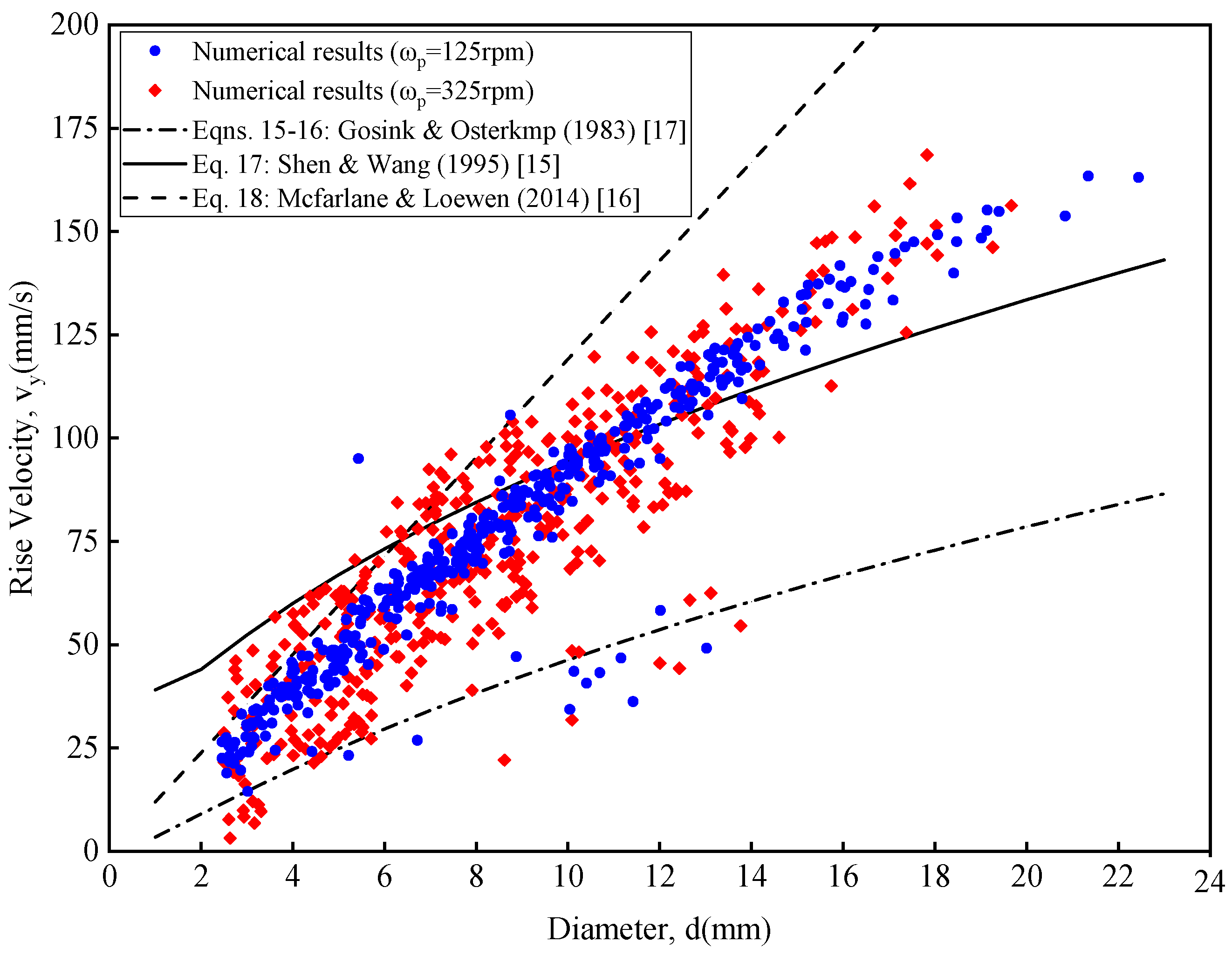
2.4. Validation of Model Accuracy

To validate the accuracy of the CFD-DEM coupling model, the numerically simulated rise velocities of frazil ice with different diameters were compared with the theoretical results calculated using the equations proposed by Gosink and Osterkamp [17], Shen and Wang [15], and Mcfarlane and Loewen [16]. The expressions for these theoretical equations are as follows:

$$v_y=\sqrt{2g^{\prime }t/C_D}$$

(15)

$$\log C_D=1.386-0.892\log Re+0.111{\left(\log Re\right)}^2$$

(16)

$$v_y=-4{\displaystyle \frac{k_2}{k_1}}{\displaystyle \frac{\nu }{d}}+\sqrt{{\left(4{\displaystyle \frac{k_2}{k_1}}{\displaystyle \frac{\nu }{d}}\right)}^2+{\displaystyle \frac{4}{3k_1}}{g}^{\prime }d}$$

(17)

$$v_y={\left[{\displaystyle \frac{\pi g^{\prime }t}{3.28}}\sqrt{{\displaystyle \frac{d}{2\nu }}}\right]}^{2/3}$$

(18)

where $v_y$ denotes the rise velocity of frazil ice, m/s; $g^{\prime }$ is the reduced gravitational acceleration, m/s², given by $g^{\prime }=g\left({\rho }_f-{\rho }_i\right)/{\rho }_f$; the frazil ice is disk-shaped; $t$ represents the thickness of the frazil ice particle, m; $d$ is the diameter of the frazil ice particle, m; $Re=v_{y}d/\nu$ is the Reynolds number for the frazil ice particle; $\nu$ is the kinematic viscosity of water at 0 °C, $1.8\times {10}^{-6}$ m²/s; and $k_1=1.22$ and $k_2=4.27$.

The computational parameters in this simulation were set according to Mcfarlane’s experiment [16] on the rise velocity of frazil ice. The computational domain is a water tank with dimensions of 1.2 × 0.8 × 1.5 m, and a water depth of 1.3 m (water density, ${\rho }_f=998.2$ kg/m³; water dynamic viscosity, ${\eta }_w=0.001$ Pa∙s). Four propellers at the bottom of the tank generate turbulence, simulating two different conditions at speeds of 125 and 325 rpm, respectively. Initially, the propellers were rotated at a set speed for 1 min to generate turbulence in the tank. Afterward, the propellers were stopped, allowing the turbulence to dissipate for 2 min. Subsequently, 450 frazil ice particles were generated in the water within 1 s, and the simulation was conducted for 20 s. The particles (particle density, ${\rho }_i$ = 917 kg/m³; particle Poisson’s ratio, ${\upsilon }_i=0.33$; particle Young’s modulus, $E=3.298\times {10}^3$ Mpa) had diameters ranging from 2.5 mm to 22.4 mm, following a log-normal distribution, with an average diameter of 8.71 mm and a standard deviation of 3.84 mm. The particle-size-to-thickness ratio was set to 10. The comparison between the numerical simulation results and the theoretical solutions is shown in Figure 1.

The numerical results align well with the results of the theoretical equations proposed by Shen and Wang [15] (Equation (17)). Additionally, variations in propeller speed did not significantly affect the frazil ice’s rise velocity. Nearly all data points fall between the theoretical solution curve of Mcfarlane and Loewen [16] (Equation (18)) for an aspect ratio of 10 and the theoretical solution curve of Gosink and Osterkamp [17] (Equations (15) and (16)) for an aspect ratio of 80, which is consistent with the experimental conclusions of Mcfarlane and Loewen [16].These findings validate that the CFD-DEM coupling method can accurately simulate the transport dynamics of frazil ice and can be utilized for studying its spatiotemporal evolution characteristics.

3. Calculation Settings

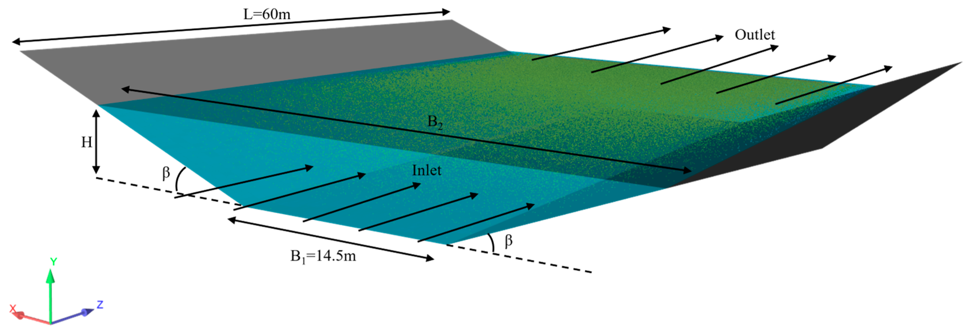
3.1. Model Setup

The channel model in this study is based on the prototype dimensions of the straight channel section of the South-to-North Water Transfer Middle Route Main Canal. The conventional cross-section of the straight channel section is trapezoidal, as shown in Figure 2. The channel bottom width $B_1$ is 14.5 m, the side slope ratio $m$ is 2.5, and the length $L$ is 60 m. Due to varying water depths, the channel surface width ranges from 29.5 to 49.5 m. To simulate the flow in the channel, the inlet is set as a velocity boundary condition with flow velocity $v$. The area above the water surface is air, and both the outlet boundary and upper boundary are set as pressure outlets. Simulation parameters are listed in

Table 2. Input parameters for the CFD-DEM numerical simulation.

Parameters	Value	Parameters	Value
Particle diameter, d (m)	0.01	$\mathrm{Water}\mathrm{density},{\rho }_w$ (kg/m3)	1000
$\mathrm{Particle}\mathrm{density},{\rho }_i$ (kg/m3)	917	$\mathrm{Water}\mathrm{dynamic}\mathrm{viscosity},{\eta }_w$ (Pa∙s)	0.001
$\mathrm{Particle}\mathrm{shear}\mathrm{modulus},G$ (MPa)	$1.24\times {10}^9$	Particle Young’s modulus, E (MPa)	$3.298\times {10}^9$
$\mathrm{Coefficient}\mathrm{of}\mathrm{restitution},c_{nrest}\mathrm{and}{c}_{trest}$	0.2	Gravitational acceleration, g (m/s2)	9.81
$\mathrm{DEM}\mathrm{timestep}\mathrm{size},\mathsf{\Delta }{t}_i$ (s)	$5\times {10}^{-6}$	$\mathrm{CFD}\mathrm{timestep}\mathrm{size},\mathsf{\Delta }{t}_w$ (s)	$5\times {10}^{-4}$
Coefficient of static friction (particle to particle)	0.42	Coefficient of static friction (particle to channel bed)	0.41
Coefficient of rolling friction (particle to particle)	0.04	Coefficient of rolling friction (particle to channel bed)	0.04
Surface energy (particle to particle)	15.60	Surface energy (particle to channel bed)	1.00

, and frazil ice particles are modelled as 10 mm-diameter spheres.

3.2. Arrangement of Simulation Schemes

This study uses the CFD-DEM coupling method to investigate the influence of the frazil ice generation rate (V_f), water flow velocity ($v$), and water depth (H) on frazil ice transport dynamics during the early stages of freezing in water conveyance channels. The frazil ice generation rate is defined as the volume of frazil ice generated per unit heat exchange area per unit time. Furthermore, expressions describing the spatiotemporal evolution of frazil ice in relation to relevant factors were derived. The values of the three factors were divided into five groups each. The frazil ice generation rate was estimated from historical meteorological data using Ashton’s linear heat exchange model [41], with values ranging from 260 to 1310 mm³/m²·s. The water flow velocity varied from 0.5 to 0.9 m/s, while the water depth ranged from 3 to 7 m, aligned with actual hydraulic conditions.

Table 3. Setting of influencing parameter values.

No.	Frazil Ice Generation Rate Vf [mm3/(m2·s)]	$\mathbf{Water}\mathbf{Flow}\mathbf{Velocity}\mathit{v}$(m/s)	Water Depth H (m)
1	260	0.50	3.00
2	520	0.60	4.00
3	780	0.70	5.00
4	1050	0.80	6.00
5	1310	0.90	7.00

summarizes the parameter values, and different combinations of these values resulted in a total of 125 simulation schemes.

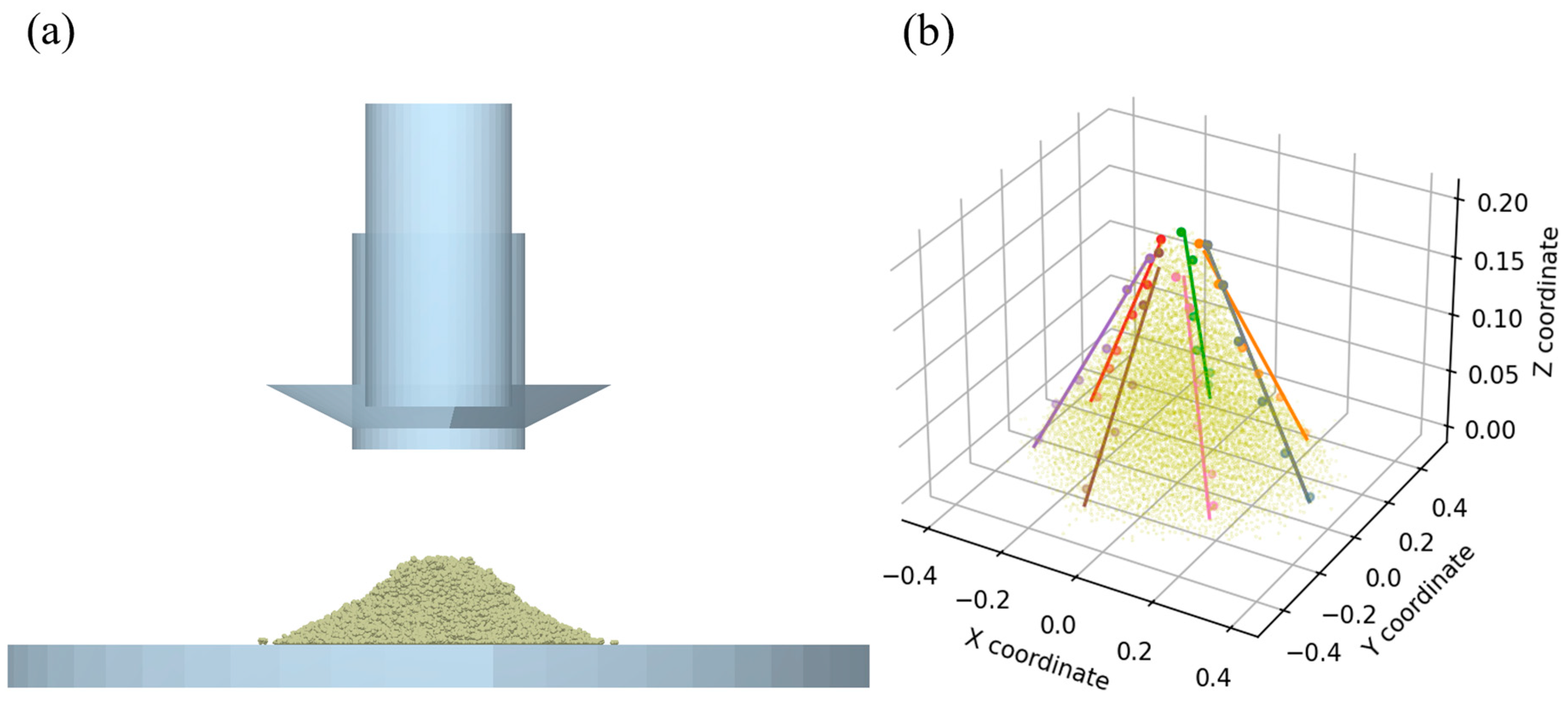
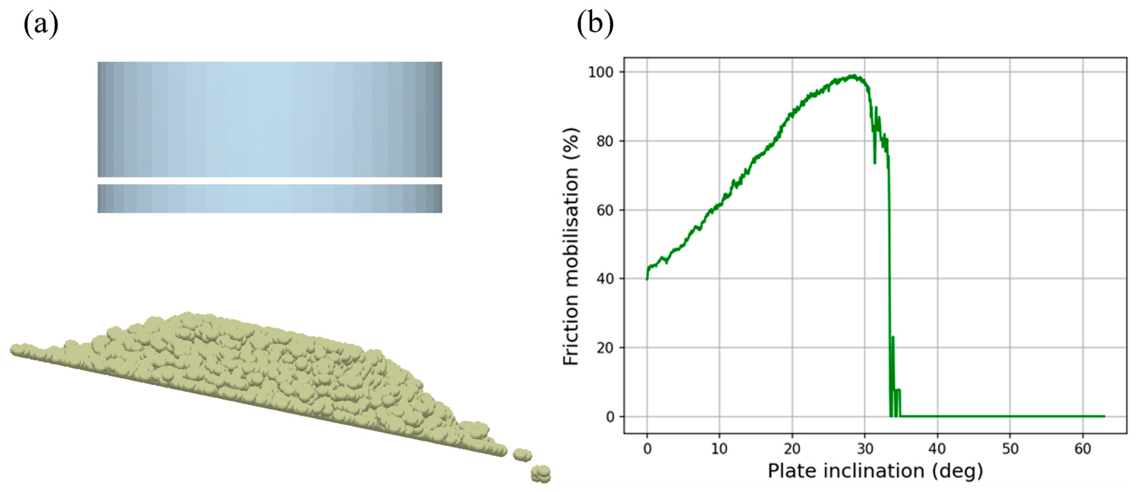
3.3. Calibration of Contact Parameters

In DEM, the mechanical behavior of each element is controlled by the specified micro-parameters. Therefore, inputting accurate micro-parameters is the key to improving the accuracy of the CFD-DEM coupled model. The micro-parameters are divided into two types: intrinsic physical parameters and contact parameters. The intrinsic physical parameters, such as size, density, and elastic modulus, are easy to obtain, while the contact parameters need to be obtained through simulation experiments. Researchers commonly calibrate the contact parameters between particles by comparing the simulated repose angle with the experimental values, adjusting the parameters to achieve a closer match. Contact parameters between particles and walls are calibrated using the sliding angle. In this study, the intrinsic physical parameters of frazil ice were based on the actual physical properties of ice. However, due to the limited application of DEM in river ice dynamics, there is a lack of suitable reference values for the contact parameters of frazil ice in DEM simulations. Therefore, we calibrated the contact parameters between frazil ice particles and between frazil ice and the channel bed through static repose angle simulations and slope sliding simulations, including the static friction coefficient, rolling friction coefficient, and surface energy. The static repose angle simulation was conducted using the cylinder lifting method, as shown in Figure 3. A bottomless cylinder was filled with a certain quantity of particles and gradually lifted. The particles slid downward due to gravity, forming a cone, and the slope angle of the cone represented the repose angle of the particle pile. Using Python, multiple radial box arrays were defined around the particle pile to identify the highest particle in each box. The coordinates of these particles’ centroids were linearly fitted using the least squares method, and the angle between the fitted line and the horizontal plane was the repose angle of the frazil ice particle pile. The slope sliding simulation used the sliding angle to calibrate the contact parameters between frazil ice and the channel bed, as shown in Figure 4. First, a bottomless cylinder was filled with a certain quantity of particles and compacted. After lifting the cylinder and allowing the particles to stabilize, the inclined plate was rotated at a constant, low angular velocity. Python was used to extract the percentage of sliding particles in contact with the inclined plate at various tilt angles, with 85% serving as the standard for determining the sliding angle.

Previous researchers have measured the repose angle of ice particle accumulations as 30.3° through static piling tests, and the sliding angle between ice blocks and the channel bed structure as 19.5° through inclined plane sliding tests. Based on existing research, the ranges and values of the experimental factors that need to be calibrated in this study are shown in

Table 4. Simulation test factor values.

Group	Factors
	Static Friction Coefficient A	Rolling Friction Coefficient B	Surface Energy C (J/m2)
Particle to particle	0.2	0.01	8
	0.3	0.02	12
	0.4	0.03	16
	0.5	0.04	20
Particle to channel bed	0.2	0.02	0
	0.3	0.03	4
	0.4	0.04	8
	0.5	0.05	12
	0.6	0.06	16

. Various combinations of parameter values were used to create different conditions, and simulations were conducted to measure the repose angle or sliding angle. The static repose angle simulation and the inclined plane sliding simulation are mutually independent, with no parameter interaction between them.

The relative error $\delta$ between the simulation results and measured values is taken as the objective, and a multiple regression fitting of the obtained data is conducted to derive a quadratic regression equation of each factor’s influence on $\delta$. The relative error $\delta$ is calculated as follows:

$$\delta ={\displaystyle \frac{\mid {\theta }^{\prime }-\theta \mid }{\theta }}\times 100\%$$

(19)

where ${\theta }^{\prime }$ denotes the simulated value, while $\theta$ denotes the measured value.

The quadratic regression equations for the effect of various factors on the relative error of the repose angle and the sliding angle are shown in Equations (20) and (21), respectively. The coefficients of determination R² values are 0.9450 and 0.9671, the adjusted coefficients of determination $R_{adj}^2$ are 0.9321 and 0.9537, and the coefficients of variation CV are 2.0% and 3.7%, which indicated that the fitted regression equations have a high accuracy and reliability. Based on this, the optimal combination of factors was determined using the response surface optimization method, with the minimum relative error as the optimization objective, as shown in

Table 5. Optimized contact parameters.

Group	Factors
	Static Friction Coefficient A	Rolling Friction Coefficient B	Surface Energy C (J/m2)
Particle to particle	0.42	0.04	15.60
Particle to channel bed	0.41	0.04	1.00

. The repose angle and sliding angle obtained from the simulations using the optimized parameters were 30.21° and 19.44°, respectively. The errors compared to the measured values were both 0.3%, indicating that the calibrated contact parameters are highly reliable:

$${\delta }_1=3.56-2.03A-1.13B-1.56C+0.5878\mathrm{A}B+2.55AC+0.5825BC-1.12A^2+1.63B^2+5.34C^2$$

(20)

$${\delta }_2=3.36-0.6923A+3.95B+4.55C-3.53\mathrm{A}B-1.26AC+10.26BC+2.05A^2+35.85B^2+1.06C^2$$

(21)

where A represents the static friction coefficient, defined as the ratio of the maximum static friction force to the normal force between two surfaces in contact; B represents the static friction coefficient, defined as the ratio of the rolling friction force to the normal force; and C represents the surface energy, defined as the energy per unit area required to separate two surfaces.

4. Results

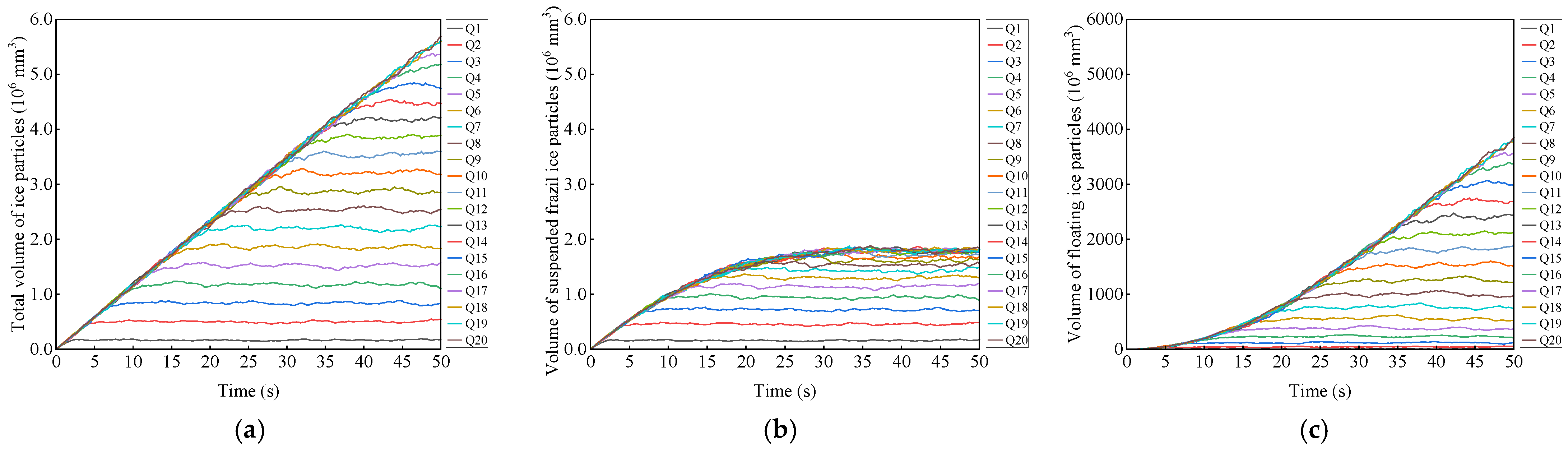
4.1. The Temporal Evolution Characteristics of Frazil Ice

To analyze the characteristics of the spatiotemporal distribution of frazil ice caused by the hydrodynamic transport of frazil ice, the channel was divided into 30 segments of 2 m in length. The curves of the change process of the total ice particle volume, the volume of suspended frazil ice, and the volume of floating ice were extracted for each channel segment. Taking the conditions of an ice generation rate of 1310 mm³/(m²·s), a flow velocity of 0.7 m/s, and a water depth of 6 m as an example, the temporal evolution of ice particle volume in the first 20 segment is shown in Figure 5 (Qi represents the i-th channel segment). Initially, the channel contained no ice, and the newly formed frazil ice particles were transported downstream by the water flow. The results show that the total volume of ice, the volume of suspended frazil ice, and the volume of floating ice in each segment increased over time, eventually reaching a stable state. The growth rate of the total ice volume in each segment remains constant over time, while the growth rate of suspended frazil ice gradually decreases, and the growth rate of floating ice increases. Segments closer to the downstream reach stability in total ice volume and floating ice volume earlier, whereas the time at which the suspended frazil ice volume stabilizes is roughly the same for most segments.

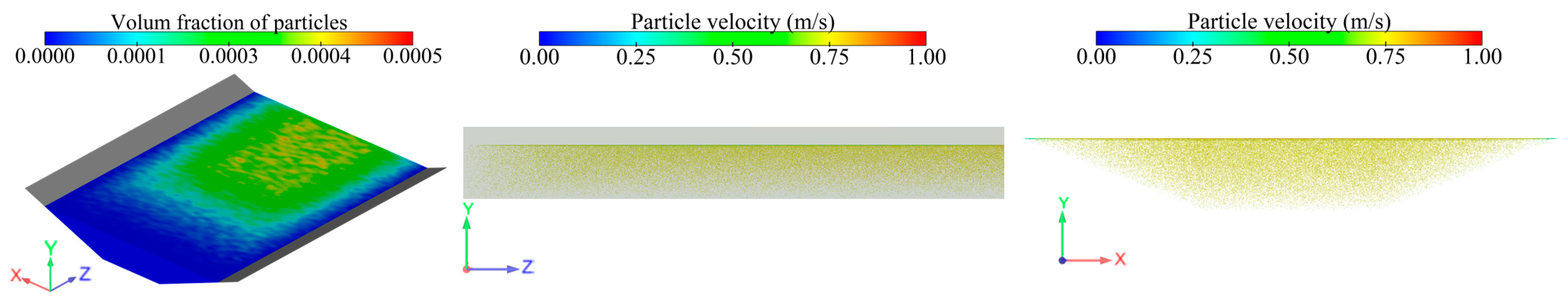
4.2. The Spatial Evolution Characteristics of Frazil Ice

Figure 6 displays the volumetric fraction contour of ice particles in the water at the end of the simulation, along with particle distribution diagrams from different perspectives. It is observed that most frazil ice has floated to the surface of the water, forming floating ice. The floating ice continuously moves downstream, resulting in a gradual increase in its amount along the channel. At the end of the simulation, the total ice volume, suspended frazil ice volume, and floating ice volume for each channel segment are presented in Figure 7. In most segments, the ice particle volume has reached a stable state, with the total ice volume showing a linear relationship with the distance along the channel. The suspended frazil ice volume remains nearly constant across most segments, while the floating ice volume also displays a linear relationship with the distance. The growth rate of floating ice aligns with the growth rate of the total ice volume, indicating that the increase in total ice is primarily driven by the floating ice. Each scheme was simulated for only 50 s. By the end of the simulation, the initially formed floating ice had not entirely transported to the downstream boundary, resulting in the total ice volume and floating ice volume in some downstream segments not reaching stable values. Additionally, in segments near the upstream boundary, the stable suspended frazil ice volume is lower than in other downstream segments, with notable variation between these segments. The floating ice volume in these segments exhibits a curved growth pattern with a slower growth rate than others. This phenomenon can be explained as follows: under these conditions, frazil ice at the channel bottom takes about 30 s to float to the water’s surface, traveling approximately 22 m downstream during this period. This distance coincides with the total length of the upstream segments, indicating that these segments’ total length represents the critical longitudinal distance required for suspended frazil ice to reach a stable state. Therefore, in the subsequent discussion, these segments will be excluded. Instead, the focus will be on segments where the floating ice volume shows steady growth and the suspended frazil ice volume becomes consistent. This approach will provide a more precise analysis of the spatiotemporal evolution pattern of frazil ice.

5. Discussions

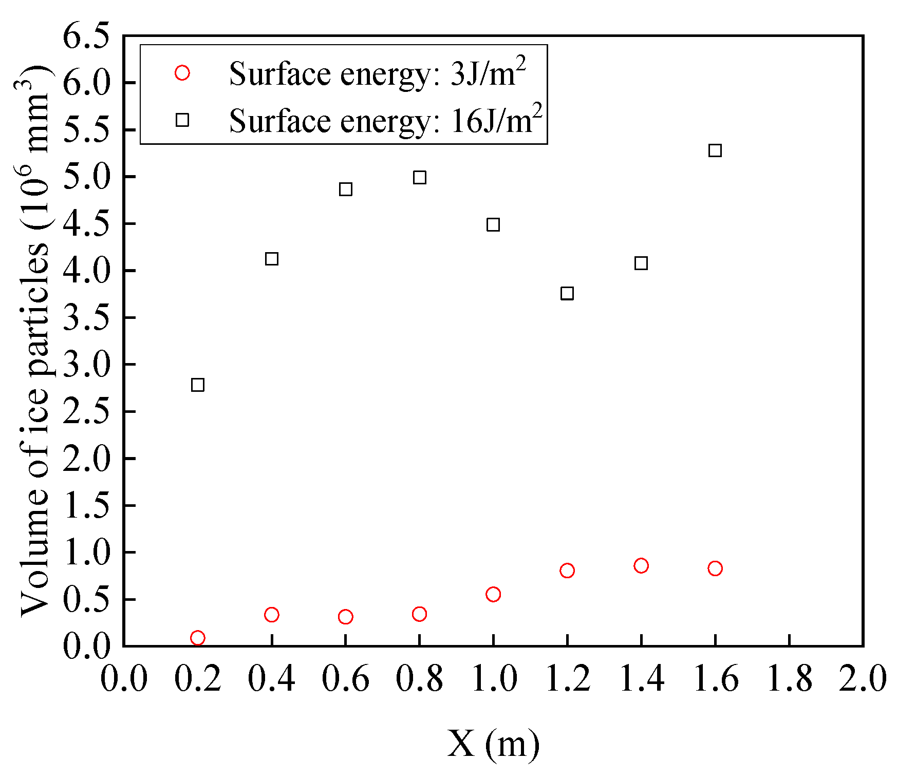
5.1. The Effect of Contact Parameters

In order to further analyze the impact of different contact parameters on the spatiotemporal evolution of ice, three sets of contact parameters are obtained based on the quadratic regression Equations (20) and (21) for the relative errors $\delta$ (${\delta }_1$ and ${\delta }_2$). These parameter sets correspond to combinations of parameters for which the relative errors ${\delta }_1$ and ${\delta }_2$ are −50%, +50%, and the minimum, respectively. The optimized set of contact parameters corresponding to the minimum value of $\delta$ is listed in Table 5. Simulations of frazil ice transport were carried out under the three sets of contact parameters. Using the control variable method, the frazil ice generation rate was set at 1310 mm³/(m²·s), the flow velocity at 0.7 m/s, and the water depth at 6 m. The contact parameters for the three schemes are shown in

Table 6. Parameter values for different contact parameter combinations.

Group	Type	Static Friction Coefficient	Rolling Friction Coefficient	Surface Energy C (J/m2)	Static Repose Angle (°)	Sliding Angle (°)
1	particle to particle	0.052	0.010	4.061	15.15	—
	particle to channel bed	0.271	0.043	5.568	—	9.75
2	particle to particle	0.420	0.040	15.600	30.21	—
	particle to channel bed	0.410	0.040	1.000	—	19.44
3	particle to particle	0.210	0.038	27.960	45.45	—
	particle to channel bed	0.545	0.040	2.088	—	29.25

.

The numerical results under the three schemes were compared to analyze the effect of contact parameters on ice spatiotemporal evolution. Figure 8 shows the simulation results of the total volume of ice particles, suspended frazil ice volume, and floating ice volume under various conditions. It can be seen that there is no significant difference in the spatiotemporal evolution of frazil ice under different contact parameter groups. This is likely because the study primarily simulates the transport process of frazil ice in the water conveyance channel during the early freezing stage of winter ice formation, where the ice concentration is low. The ice concentration is expressed as the ratio of ice volume to water volume in a single segment of the channel. The maximum ice concentration under all conditions is just 0.0017%, significantly reducing the likelihood of collisions and adhesion during frazil ice movement. As a result, the spatiotemporal evolution of frazil ice is largely unaffected by contact parameters.

However, for simulations involving ice jam formation and breakage, the contact parameters may have a greater impact on the simulation results. Accordingly, we input the calibrated static and rolling friction coefficients, and simulated ice jam formation caused by floating ice accumulation upstream of the siphon using surface energies of 3 J/m² and 16 J/m² for two conditions. The maximum ice concentration in the two conditions is 9.59%. Figure 9 illustrates the volume of ice particles at the front edge of the inverted siphon inlet when the ice jam reaches a stable state under the two conditions. The results show a significant difference, with the higher surface energy exhibiting a notably larger amount of ice particles. Therefore, contact parameters significantly impact the simulation results of ice jams in water conveyance channels. In the following chapters, we will only discuss the spatiotemporal evolution of frazil ice during the early freezing stage of winter when the ice concentration is low and ice jams do not occur.

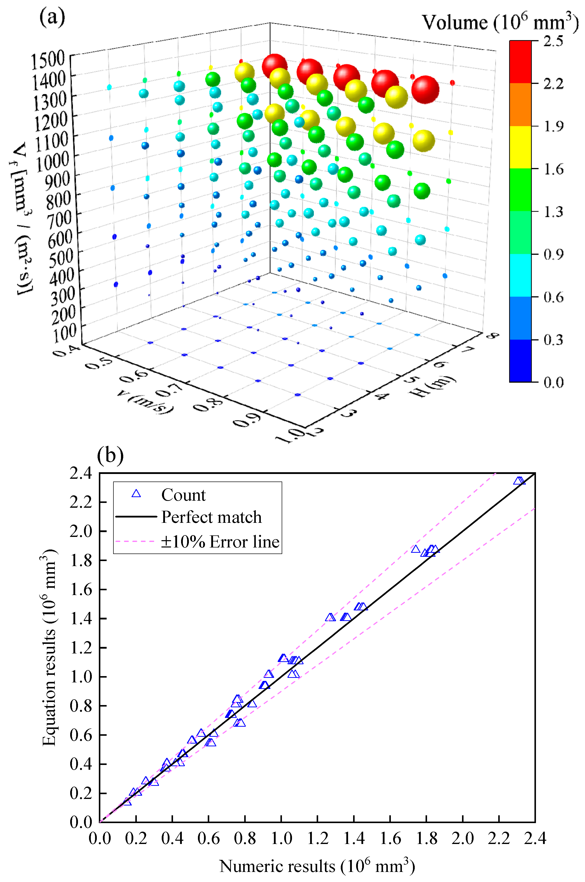
5.2. Analysis of the Evolution Pattern of the Volume of Suspended Frazil Ice

As previously noted, the stable volume of suspended frazil ice shows no significant spatial variation. To further analyze the spatiotemporal evolution dynamics of suspended frazil ice, the stable volume for each segment was averaged and used as the stable volume for any individual segment. Figure 10a shows the numerical simulation results of the stable volume of suspended frazil ice in a single segment under different simulation conditions. It can be observed that the stable volume of suspended frazil ice increases with the frazil ice generation rate and water depth, but does not change with flow velocity. This can be explained by the mass conservation principle during the frazil ice transport process. The transport of suspended frazil ice occurs in two directions: vertically and along the flow. At a constant flow velocity, some of the suspended frazil ice in any given segment rises to the surface or is carried downstream, while ice particles from upstream are transported into the segment to compensate for the ice transported downstream. Thus, the suspended frazil ice volume is independent of the flow velocity.

In order to obtain a rapid prediction method for ice conditions in water conveyance channels, it is necessary to analyze and derive the relational equations between the spatiotemporal evolution of frazil ice and associated factors. Assuming that, after every $\mathsf{\Delta }t$ time interval, a proportion $k$ of the suspended frazil ice in the channel rises to the surface, $k$ can be expressed by Equation (22). Although some ice particles are transported downstream to other segments, an equal amount of ice is transported from upstream into the segment, so the proportion of suspended frazil ice retained in the segment is $\left(1-k\right)$. Therefore, the suspended frazil ice volume in any segment at time $t_0+n\mathsf{\Delta }t$ can be derived, as expressed in Equation (23). The volume of frazil ice generated in a segment of length $dx$ during time $\mathsf{\Delta }t$ can be expressed by Equation (24), where $v_y$ is the rise velocity of frazil ice. Equation (23) is valid when $\mathsf{\Delta }t$ approaches 0, but the prediction results obtained from this equation still exhibit considerable deviations from the numerical simulation results. Therefore, we introduce a coefficient $\alpha =0.65$ to derive a more accurate prediction formula for the volume of suspended frazil ice, as presented in Equation (25):

$$k={\displaystyle \frac{\left(B_1+2mH-mdH\right)dH}{\left(B_1+mH\right)H}}$$

(22)

$$S_n=V\left[{\left(1-k\right)}^0+{\left(1-k\right)}^1+{\left(1-k\right)}^2+\cdots \cdots +{\left(1-k\right)}^{n-1}\right]\approx {\displaystyle \frac{V}{k}}$$

(23)

$$V={\displaystyle \frac{V_f\left(B+2mH\right)dxdH}{v_y}}$$

(24)

$$S_n=\alpha {\displaystyle \frac{V_f\left(B+mH\right)Hdx}{v_y}}$$

(25)

The scatter plot of the predicted and numerical results is shown in Figure 10b. The absolute percentage error (APE) between the predicted and numerical results is calculated using the following formula:

$$\mathrm{APE}=\left|{\displaystyle \frac{{\mathrm{Results}}_{eq}-{\mathrm{Results}}_{sim}}{{\mathrm{Results}}_{sim}}}\right|\times 100\%$$

(26)

An APE of less than 20% is deemed reasonable and practical for engineering purposes. The maximum APE between the theoretical solution from Equation (25) and the numerical solution is 13.24%. In 76% of the cases, the APE is less than ±10%, and the mean absolute percentage error (MAPE) is 6.32%. Therefore, it can be concluded that Equation (25) offers a relatively reliable prediction for the suspended frazil ice volume in water conveyance channels.

The production of frazil ice in river channels is primarily influenced by thermal factors, which are manifested through heat loss caused by heat exchange between the water and the external environment. The heat loss at the water surface can be calculated using detailed heat exchange equations [42,43,44]. Considering the heat exchange area between the water and the atmosphere, the frazil ice generation rate can be expressed using the following equation [45]:

$$V_f={\displaystyle \frac{\sum \varphi }{{\rho }_i{C}_i}}$$

(27)

where $\sum \varphi$ represents the heat exchange flux between the water and the external environment, W/m²; ${\rho }_i$ denotes the density of ice, kg/m³; and $C_i$ stands for the latent heat of freezing, J/kg.

Therefore, the prediction formula for the evolution of suspended frazil ice in the channel can be further rewritten as follows:

$$S_n=\alpha {\displaystyle \frac{\left(B+mH\right)H\sum \varphi dx}{{\rho }_i{C}_i{v}_y}}$$

(28)

5.3. Analysis of the Evolution Pattern of Total Volume of Ice and the Volume of Floating Ice

The evolution of the total ice volume in each segment with respect to the frazil ice generation rate, water flow velocity, and water depth is shown in Figure 11. Figure 11a illustrates the influence of the frazil ice generation rate on the spatial distribution of the total ice volume, where a higher frazil ice generation rate leads to a greater amount of ice in each segment. Figure 11b indicates that, with a higher water flow velocity, frazil ice is transported downstream more quickly, leading to a smaller amount of ice in each segment at stabilization. The numerical simulation results in Figure 11c demonstrate that, as the water depth increases, the total ice volume in each segment increases correspondingly. In summary, the total ice volume in each segment is positively correlated with both the frazil ice generation rate and water depth but negatively correlated with the water flow velocity.

During the transport process, the total volume of ice particles in each segment mainly comes from ice particles transported upstream and those generated within the current segment. Assuming that the frazil ice production in a single segment during time $\mathsf{\Delta }t$ is $N$ (as shown in Equation (30)), and, after each $\mathsf{\Delta }t$, the ice particles travel a longitudinal distance equal to one segment length, $dx$, then, after $\mathsf{\Delta }t$, the frazil ice in each segment will be entirely transported to the downstream segment. Therefore, once the channel begins generating ice, the total volume of ice particles in one segment reaches a stable value after each $\mathsf{\Delta }t$. If the channel starts generating ice at time $t_0$, the total volume of ice particles in the $n$-th segment stabilizes at $t_0+n\mathsf{\Delta }t$, and its stable value can be expressed by Equation (31). By incorporating Equation (27), Equation (31) can be rewritten in the form of Equation (32):

$$\mathsf{\Delta }t={\displaystyle \frac{dx}{v}}$$

(29)

$$V={\displaystyle \frac{V_f\left(B_1+2mH\right)d{x}^2}{v}}$$

(30)

$$Q_n=nV={\displaystyle \frac{n{V}_f\left(B_1+2mH\right)d{x}^2}{v}}$$

(31)

$$Q_n={\displaystyle \frac{n\left(B_1+2mH\right)\sum \varphi d{x}^2}{{\rho }_i{C}_{i}v}}$$

(32)

The comparison between the predicted results from Equation (31) and the numerical results is shown in Figure 12. The color of the points indicates the magnitude of the Normalized Mean Absolute Error (NMAE) and Normalized Root Mean Square Error (NMSE) between the theoretical solution and the simulation results, where values closer to 0 indicate a greater accuracy of the theoretical solution. The calculation formulae for NMAE and NMSE are as follows:

$$\mathrm{NMAE}={\displaystyle \frac{\frac{1}{n}{{\displaystyle \sum }}_{i=1}^n\frac{\left|{\mathrm{Results}}_{eq}-{\mathrm{Results}}_{sim}\right|}{{\mathrm{Results}}_{sim}}}{\overline{{\mathrm{Results}}_{sim}}}}\times 100\%$$

(33)

$$\mathrm{NMSE}={\displaystyle \frac{\sqrt{\frac{1}{n}{{\displaystyle \sum }}_{i=1}^n{\left({\mathrm{Results}}_{eq}-{\mathrm{Results}}_{sim}\right)}^2}}{\overline{{\mathrm{Results}}_{sim}}}}\times 100\%$$

(34)

where ${\mathrm{Results}}_{eq}$ represents the calculated value of the objective function; ${\mathrm{Results}}_{sim}$ denotes the calculated value from the numerical simulation; and $\overline{{\mathrm{Results}}_{sim}}$ is the mean value of the numerical simulation results

The maximum NMAE and NMSE are 9.931% and 9.546%, respectively, with all results having NMAE and NMSE within 10%, which indicates that the proposed Equation (31) provides a high accuracy and reliability for predicting the spatial distribution of frazil ice in long-distance river channels.

Based on the previous analysis and derivation of the spatiotemporal evolution of suspended frazil ice and the total volume of ice during transport, we can derive the prediction formula for the floating ice volume in the $n$-th segment (as shown in Equation (35)), with the increase in floating ice relative to the $\left(n-1\right)$-th segment expressed by Equation (36). Figure 13a shows the difference in floating ice volume between two adjacent segments under different conditions. It can be seen that the increase in floating ice is positively correlated with the frazil ice generation rate and water depth and negatively correlated with the flow velocity. Figure 13b compares the predicted surface floating ice increase from Equation (36) with the numerical simulation results. The APE between the theoretical and numerical results is less than ±10% for all cases, with a maximum of 7.80% and an average percentage error (MAPE) of 2.89%, proving the accuracy of the prediction from Equation (36):

$$F_n=Q_n-S_n={\displaystyle \frac{n{V}_f\left(B_1+2mH\right)d{x}^2}{v}}-\alpha {\displaystyle \frac{V_f\left(B+mH\right)Hdx}{v_y}}$$

(35)

$$\mathsf{\Delta }{F}_n={\displaystyle \frac{V_f\left(B_1+2mH\right)d{x}^2}{v}}$$

(36)

According to Equation (27), the stable value of the floating ice volume and its growth in the $n$-th segment can be rewritten in the forms of Equations (37) and (38), respectively:

$$F_n={\displaystyle \frac{n\left(B_1+2mH\right)\sum \varphi d{x}^2}{{\rho }_i{C}_{i}v}}-\alpha {\displaystyle \frac{\left(B+mH\right)H\sum \varphi dx}{{\rho }_i{C}_i{v}_y}}$$

(37)

$$\mathsf{\Delta }{F}_n={\displaystyle \frac{\sum \varphi \left(B_1+2mH\right)d{x}^2}{{\rho }_i{C}_{i}v}}$$

(38)

6. Conclusions

This study establishes a frazil ice motion model using the CFD-DEM coupling method and calibrates the model’s contact parameters through static repose angle simulations and slope sliding simulations. Building on this, a three-dimensional numerical simulation was conducted on the process of frazil ice transport during the initial freezing stages in water conveyance channels, analyzing the influence of multiple factors on the spatiotemporal evolution of frazil ice and developing a rapid prediction method for its spatiotemporal evolution. The main research findings are as follows:

(1)

In conditions characterized by a low ice concentration, such as the transport of frazil ice during the early freezing stages in water conveyance channels, the contact parameters have no significant effect on the simulation results. In contrast, the influence of contact parameters is significant for simulations of ice phenomena with high ice concentrations, such as ice jam formation and breakage.

(2)

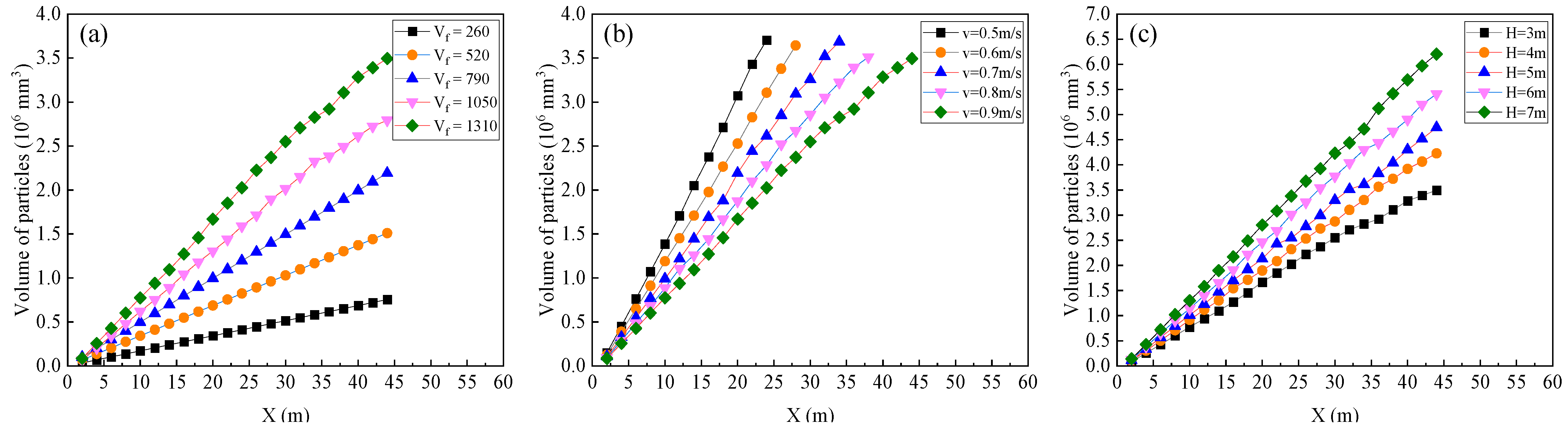
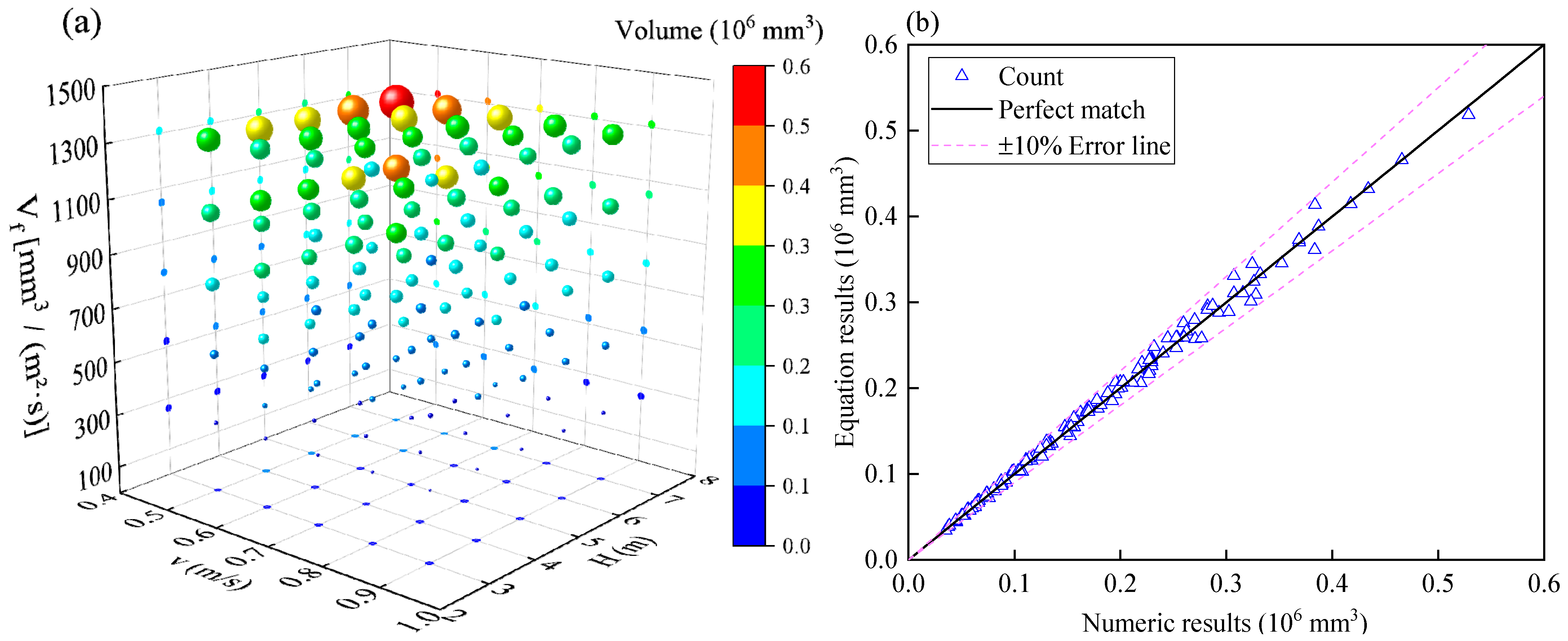
A prediction formula for the spatiotemporal evolution of the suspended frazil ice amount in water conveyance channels has been proposed. The predicted results closely match the numerical results, with a maximum APE of 13.24%, a MAPE of 6.32%, and 76% of the theoretical solutions falling within the error line of ±10%. The suspended frazil ice amount is positively correlated with the frazil ice generation rate and water depth while negatively correlated with the rise velocity of frazil ice, exhibiting minimal influence from the water flow velocity.

(3)

Prediction formulae for the evolution of total ice amount and floating ice amount in water conveyance channels have been proposed. The maximum NMAE for the total ice amount predicted results is 9.931%, and the maximum NMSE is 9.546%. The floating ice amount increases linearly along the channel, with a maximum APE of 7.80% between the predicted and numerical results for the increase in floating ice and an average MAPE of 2.89%. The increase in floating ice is positively correlated with the frazil ice generation rate and water depth while negatively correlated with the water flow velocity.

This research contributes to enhancing the timeliness of ice condition predictions in water conveyance projects, providing a theoretical basis for the efficient switching of water conveyance modes during the ice period. And it holds significant importance for regulating ice conditions and preventing ice damage in water conveyance channels.

References

1. Hicks, F. An overview of river ice problems: CRIPE07 guest editorial. Cold Reg. Sci. Technol. 2009, 55, 175–185. [Google Scholar] [CrossRef]
2. Beltaos, S.; Prowse, T.D.; Carter, T. Ice regime of the lower Peace River and ice-jam flooding of the Peace-Athabasca Delta. Hydrol. Process. 2006, 20, 4009–4029. [Google Scholar] [CrossRef]
3. Makkonen, L.; Tikanmäki, M. Modelling frazil and anchor ice on submerged objects. Cold Reg. Sci. Technol. 2018, 151, 64–74. [Google Scholar] [CrossRef]
4. Schaefer, V.J. The formation of frazil and anchor ice in cold water. Eos Trans. Am. Geophys. Union 1950, 31, 885–893. [Google Scholar] [CrossRef]
5. Hanley, T.; Michel, B. Temperature patterns during the formation of border ice and frazil in a laboratory tank. In Proceedings of the 3rd International Symposium on Ice Problems, Hanover, NH, USA, 18–21 August 1975; pp. 18–21. [Google Scholar]
6. Hanley, T.O.D.; Michel, B. Laboratory formation of border ice and frazil slush. Can. J. Civ. Eng. 1977, 4, 153–160. [Google Scholar] [CrossRef]
7. Clark, S.; Doering, J. Laboratory Experiments on Frazil-Size Characteristics in a Counterrotating Flume. J. Hydraul. Eng. 2006, 132, 94–101. [Google Scholar] [CrossRef]
8. Clark, S.; Doering, J. Experimental investigation of the effects of turbulence intensity on frazil ice characteristics. Can. J. Civ. Eng. 2008, 35, 67–79. [Google Scholar] [CrossRef]
9. Chen, Y.; Lian, J.; Zhao, X.; Guo, Q.; Yang, D. Advances in Frazil Ice Evolution Mechanisms and Numerical Modelling in Rivers and Channels in Cold Regions. Water 2023, 15, 2582. [Google Scholar] [CrossRef]
10. Ghobrial, T.R.; Loewen, M.R.; Hicks, F.E. Characterizing suspended frazil ice in rivers using upward looking sonars. Cold Reg. Sci. Technol. 2013, 86, 113–126. [Google Scholar] [CrossRef]
11. Mcfarlane, V.; Loewen, M.; Hicks, F. Measurements of the size distribution of frazil ice particles in three Alberta rivers. Cold Reg. Sci. Technol. 2017, 142, 100–117. [Google Scholar] [CrossRef]
12. Mcfarlane, V.; Loewen, M.; Hicks, F. Field measurements of suspended frazil ice. Part II: Observations and analyses of frazil ice properties during the principal and residual supercooling phases. Cold Reg. Sci. Technol. 2019, 165, 102796. [Google Scholar] [CrossRef]
13. Wuebben, J.L. The rise pattern and velocity of frazil ice. In Proceedings of the Third Workshop on the Hydraulics of Ice Covered Rivers, Session F, Fredericton, NB, Canada, June 1984; pp. 297–316. [Google Scholar]
14. Svensson, U.; Omstedt, A. Simulation of supercooling and size distribution in frazil ice dynamics. Cold Reg. Sci. Technol. 1994, 22, 221–233. [Google Scholar] [CrossRef]
15. Shen, H.T.; Wang De, S. Under Cover Transport and Accumulation of Frazil Granules. J. Hydraul. Eng. 1995, 121, 184–195. [Google Scholar] [CrossRef]
16. Mcfarlane, V.; Loewen, M.; Hicks, F. Laboratory measurements of the rise velocity of frazil ice particles. Cold Reg. Sci. Technol. 2014, 106–107, 120–130. [Google Scholar] [CrossRef]
17. Gosink, J.P.; Osterkamp, T.E. Measurements and Analyses of Velocity Profiles and Frazil Ice-Crystal Rise Velocities During Periods of Frazil-Ice Formation in Rivers. Ann. Glaciol. 1983, 4, 79–84. [Google Scholar] [CrossRef]
18. Hammar, L.; Shen, H.T. Frazil evolution in channels. J. Hydraul. Res. 1995, 33, 291–306. [Google Scholar] [CrossRef]
19. Wang, S.M.; Doering, J.C. Numerical Simulation of Supercooling Process and Frazil Ice Evolution. J. Hydraul. Eng. 2005, 131, 889–897. [Google Scholar] [CrossRef]
20. Wang, S.M.; Doering, J.C. Development of a mathematical model of frazil ice evolution based on laboratory tests using a counter-rotating flume. Can. J. Civ. Eng. 2007, 34, 210–218. [Google Scholar] [CrossRef]
21. Abba, A.; Olla, P.; Valdettaro, L. Numerical analysis of frazil ice formation in turbulent convection. In Proceedings of the Progress in Turbulence VI: Proceedings of the iTi Conference on Turbulence 2014, Bertinoro, Italy, 21–25 October 2014; Springer: Cham, Switzerland, 2016; pp. 299–303. [Google Scholar]
22. Blackburn, J.; She, Y. A comprehensive public-domain river ice process model and its application to a complex natural river. Cold Reg. Sci. Technol. 2019, 163, 44–58. [Google Scholar] [CrossRef]
23. Liou, C.P.; Ferrick, M.G. A model for vertical frazil distribution. Water Resour. Res. 1992, 28, 1329–1337. [Google Scholar] [CrossRef]
24. Wang, J.; Li, Q.-G.; Sui, J.-Y. Floating Rate of Frazil ICE Particles in Flowing Water in Bend Channels—A Three-Dimensional Numerical Analysis. J. Hydrodyn. 2010, 22, 19–28. [Google Scholar] [CrossRef]
25. Robb, D.M.; Gaskin, S.J.; Marongiu, J.C. SPH-DEM model for free-surface flows containing solids applied to river ice jams. J. Hydraul. Res. 2016, 54, 27–40. [Google Scholar] [CrossRef]
26. Amaro Junior, R.; Mellado, A.; Shakibaeinia, A.; Cheng, L.Y. A fully Lagrangian mesh-free numerical model for river ice dynamic. In Proceedings of the 20th Workshop on the Hydraulics of Ice Covered Rivers (CRIPE), Ottawa, ON, Canada, 14–16 May 2019. [Google Scholar]
27. Ma, H.; Zhou, L.; Liu, Z.; Chen, M.; Xia, X.; Zhao, Y. A review of recent development for the CFD-DEM investigations of non-spherical particles. Powder Technol. 2022, 412, 117972. [Google Scholar] [CrossRef]
28. Cundall, P.A.; Strack, O.D.L. A discrete numerical model for granular assemblies. Géotechnique 1979, 29, 47–65. [Google Scholar] [CrossRef]
29. Hertz, H. On the Contact of Elastic Solids. Crelle’s J. 1882, 92, 156–171. [Google Scholar] [CrossRef]
30. Mindlin, R.D.; Deresiewicz, H. Elastic Spheres in Contact Under Varying Oblique Forces. J. Appl. Mech. 1953, 20, 327–344. [Google Scholar] [CrossRef]
31. Johnson, K.L.; Kendall, K.; Roberts, A.D. Surface energy and the contact of elastic solids. Proc. R. Soc. Lond. A Math. Phys. Sci. 1971, 324, 301–313. [Google Scholar]
32. Li, L.; Wang, J.; Feng, L.; Gu, X. Computational fluid dynamics simulation of hydrodynamics in an uncovered unbaffled tank agitated by pitched blade turbines. Korean J. Chem. Eng. 2017, 34, 2811–2822. [Google Scholar] [CrossRef]
33. Anderson, T.B.; Jackson, R. Fluid Mechanical Description of Fluidized Beds. Equations of Motion. Ind. Eng. Chem. Fundam. 1967, 6, 527–539. [Google Scholar] [CrossRef]
34. Kloss, C.; Goniva, C.; Hager, A.; Amberger, S.; Pirker, S. Models, algorithms and validation for opensource DEM and CFD–DEM. Prog. Comput. Fluid Dyn. Int. J. 2012, 12, 140–152. [Google Scholar] [CrossRef]
35. Zhao, J.; Shan, T. Coupled CFD–DEM simulation of fluid–particle interaction in geomechanics. Powder Technol. 2013, 239, 248–258. [Google Scholar] [CrossRef]
36. Jing, L.; Kwok, C.Y.; Leung, Y.F.; Sobral, Y.D. Extended CFD–DEM for free-surface flow with multi-size granules. Int. J. Numer. Anal. Methods Geomech. 2015, 40, 62–79. [Google Scholar] [CrossRef]
37. Zhu, H.P.; Zhou, Z.Y.; Yang, R.Y.; Yu, A.B. Discrete particle simulation of particulate systems: Theoretical developments. Chem. Eng. Sci. 2007, 62, 3378–3396. [Google Scholar] [CrossRef]
38. Mei, R. An approximate expression for the shear lift force on a spherical particle at finite reynolds number. Int. J. Multiph. Flow 1992, 18, 145–147. [Google Scholar] [CrossRef]
39. Saffman, P.G. The lift on a small sphere in a slow shear flow. J. Fluid Mech. 1965, 22, 385–400. [Google Scholar] [CrossRef]
40. Shi, P.; Rzehak, R. Lift forces on solid spherical particles in unbounded flows. Chem. Eng. Sci. 2019, 208, 115145. [Google Scholar] [CrossRef]
41. Ashton, G.D. River and Lake Ice Engineering; Water Resources Publications: Littleton, CO, USA, 1986. [Google Scholar]
42. Shen, H.T.; Chiang, L.A. Simulation of Growth and Decay of River Ice Cover. J. Hydraul. Eng. 1984, 110, 958–971. [Google Scholar] [CrossRef]
43. Ashton, G.D. Deterioration of Floating Ice Covers. J. Energy Resour. Technol. 1985, 107, 177–182. [Google Scholar] [CrossRef]
44. Dugdale, S.J.; Hannah, D.M.; Malcolm, I.A. River temperature modelling: A review of process-based approaches and future directions. Earth-Sci. Rev. 2017, 175, 97–113. [Google Scholar] [CrossRef]
45. Shen, H.T. Surface heat loss and frazil ice production in the St. Lawrence river. J. Am. Water Resour. Assoc. 1980, 16, 996–1001. [Google Scholar] [CrossRef]
Figure 1. Comparison of rising velocities of frazil ice with different diameters.
Water 16 03367 g001
Figure 2. CFD-DEM numerical model for frazil ice transport.
Water 16 03367 g002
Figure 3. (a) Static repose angle simulation model, and (b) static repose angle measurement.
Water 16 03367 g003
Figure 4. (a) Inclined plane sliding simulation model, and (b) inclined plane sliding angle measurement.
Water 16 03367 g004
Figure 5. The evolution process of (a) total volume of ice particles, (b) volume of suspended frazil ice particles, and (c) volume of floating ice particles in each segment.
Water 16 03367 g005
Figure 6. Spatial distribution of ice particles at the end of the simulation.
Water 16 03367 g006
Figure 7. Longitudinal distribution of ice particles at the end of the simulation.
Water 16 03367 g007
Figure 8. Comparison of (a) stable total volume of ice, (b) stable suspended frazil ice volume, and (c) stable floating ice volume under different contact parameter combinations.
Water 16 03367 g008
Figure 9. Comparison of the volume of ice particles along the length of the ice jam under different contact parameters.
Water 16 03367 g009
Figure 10. (a) Numerical results of suspended frazil ice volume, and (b) scatter plot of theoretical and numerical solutions for suspended frazil ice volume.
Water 16 03367 g010
Figure 11. The evolution of total volume of ice with (a) frazil ice generation rate, (b) flow velocity, and (c) water depth.
Water 16 03367 g011
Figure 12. (a) Normalized Mean Absolute Error (NMAE) values between predicted results and numerical simulation results under different conditions, and (b) Normalized Root Mean Square Error (NMSE) values between predicted results and numerical simulation results under different conditions.
Water 16 03367 g012
Figure 13. (a) Simulation results of the floating ice growth, and (b) scatter plot of the theoretical and numerical solutions for floating ice growth.
Water 16 03367 g013