Seasonal WaveNet-LSTM: A Deep Learning Framework for Precipitation Forecasting with Integrated Large Scale Climate Drivers

Abstract

Seasonal precipitation forecasting (SPF) is critical for effective water resource management and risk mitigation. Large-scale climate drivers significantly influence regional climatic patterns and forecast accuracy. This study establishes relationships between key climate drivers—El Niño–Southern Oscillation (ENSO), Southern Oscillation Index (SOI), Indian Ocean Dipole (IOD), Real-time Multivariate Madden–Julian Oscillation (MJO), and Multivariate ENSO Index (MEI)—and seasonal precipitation anomalies (rainy, summer, and winter) in Eastern Thailand, utilizing Pearson’s correlation coefficient. Following the establishment of these correlations, the most influential drivers were incorporated into the forecasting models. This study proposed an advanced SPF methodology for Eastern Thailand through a Seasonal WaveNet-LSTM model, which integrates Long Short-Term Memory (LSTM) and Recurrent Neural Networks (RNNs) with Wavelet Transformation (WT). By integrating large-scale climate drivers alongside key meteorological variables, the model achieves superior predictive accuracy compared to traditional LSTM models across all seasons. During the rainy season, the WaveNet-LSTM model (SPF-3) achieved a coefficient of determination (R²) of 0.91, a normalized root mean square error (NRMSE) of 8.68%, a false alarm rate (FAR) of 0.03, and a critical success index (CSI) of 0.97, indicating minimal error and exceptional event detection capabilities. In contrast, traditional LSTM models yielded an R² of 0.85, an NRMSE of 10.28%, a FAR of 0.20, and a CSI of 0.80. For the summer season, the WaveNet-LSTM model (SPF-1) outperformed the traditional model with an R² of 0.87 (compared to 0.50 for the traditional model), an NRMSE of 12.01% (versus 25.37%), a FAR of 0.09 (versus 0.30), and a CSI of 0.83 (versus 0.60). In the winter season, the WaveNet-LSTM model demonstrated similar improvements, achieving an R² of 0.79 and an NRMSE of 13.69%, with a FAR of 0.23, compared to the traditional LSTM’s R² of 0.20 and NRMSE of 41.46%. These results highlight the superior reliability and accuracy of the WaveNet-LSTM model for operational seasonal precipitation forecasting (SPF). The integration of large-scale climate drivers and wavelet-decomposed features significantly enhances forecasting performance, underscoring the importance of selecting appropriate predictors for climatological and hydrological studies.

1. Introduction

Climate change directly impacts seasonal precipitation and its temporal distribution across Asia [1,2]. The variability of the East Asian monsoon and the complex topography pose significant barriers to the accuracy of seasonal precipitation forecasting (SPF) in Thailand [3,4,5]. Forecasting is crucial to understanding spatial and temporal instability. However, SPF presents challenges due to the interaction of several factors, including temperature, humidity, and large-scale climate drivers [6,7]. Precipitation is the product of complex atmospheric phenomena that present variability across different regions. It is widely recognized that various large-scale climatic patterns exert a significant influence on precipitation worldwide [8]. Numerous studies have interpreted these climate drivers’ impacts on Thailand’s precipitation patterns [9,10,11]. In SPF, large-scale climate variables are key factors shaping the likelihood of specific outcomes, like droughts or floodings [8,12]. The El Niño Southern Oscillation (ENSO) is an atmospheric and oceanic variation pattern that occurs every few years. It significantly impacts climate variability in tropical and subtropical areas, leading to significant weather changes [13,14,15,16]. The effects of ENSO, whether during El Niño, La Niña, or Neutral phases, can differ from country to country [17]. While the ENSO influences Thailand’s seasonal forecasts, its variability leads to unexpected results [15]. Over the past years, significant changes in precipitation patterns have been observed, attributable to both natural climate variability and anthropogenic impacts [18]. Many researchers have discussed the effects of climatic events on precipitation in various regions of Thailand [10,19,20,21,22,23]. For example, A study indicated that significant climatic events indirectly affect both total and extreme precipitation in Thailand, particularly influenced by the Pacific Ocean [24]. From 1955 to 2015, there was a noticeable decline in consecutive wet days, which corresponded with an increase in consecutive dry days [10]. During La Niña years and the cool phase of the Pacific Decadal Oscillation, consecutive dry days were generally shorter than average, whereas during El Niño years, these dry spells were prolonged [10]. Räsänen and Kummu (2013) discovered that ENSO substantially impacts the hydrology of the Mekong River, showing a strong correlation between annual precipitation changes and the ending of an ENSO phase [19]. These findings align with other studies, such as those by Singhrattna et al. (2005) and Buckley et al. (2007), which also identified a connection between El Niño events and drought conditions in Thailand [20,21]. However, the influence of ENSO on rainfall variability is complex and varies, especially when interacting with other climate patterns [22]. Additionally, Shimizu et al. (2017) showed that the concentration of extreme precipitation during El Niño years is affected by the Madden–Julian Oscillation (MJO). ENSO-related precipitation anomalies can be weakened or intensified simultaneously with the MJO [23]. These studies highlight that rainfall variability shows diverse patterns with ENSO activity. Additionally, other climatic oscillations, such as the Indian Ocean Dipole (IOD), South Indian Ocean SST Index, Southern Oscillation Index (SOI), MJO Index, and Multivariate ENSO Index (MEI), also interact with ENSO, further influencing rainfall variability [25,26,27,28]. The effects of these large-scale climate drivers on seasonal precipitation in Eastern Thailand remain largely unexplored. Consequently, developing a methodology to understand these impacts and incorporate them into SPF is essential. Different methodologies have been formulated for SPF, ranging from dynamic modeling to statistical approaches and combinations [29]. Statistical models create empirical connections between a target variable and one or more predictor variables. Their effectiveness, derived from historical data, relies on the quality of oceanic, atmospheric, and hydro-meteorological information [30]. These models imply less complex and operational costs than dynamic models [31]. Moreover, statistical models offer relative flexibility in construction and have the potential to enhance forecast lead time and predictability through the accretion of observations and related data, albeit with less stable predictability compared to dynamic models [32]. In recent years, artificial intelligence (AI), including artificial neural networks (ANNs), machine learning (ML), and deep learning (DL), has emerged as a viable solution to complexity [33]. The rapid progress of DL has highlighted its promising potential in SPF. The advent of the ‘big data’ era has increased intense shifts across various disciplines [34]. DL, a multi-layered model, can identify and learn non-linear features by elevating lower-level characteristics to more complex ones [35]. DL including ANNs [36], Long short-term memory (LSTM) [37,38,39], Recurrent neural networks (RNN) [11], graph neural networks (GNN) [40], conventional neural networks (CNN) [41], Transformer Neural Network (TNN) [42], decision trees (DTs) [43], wavelets decompositions with ML or DL models [44,45] are some of the most widely used AITs for precipitation forecasting [33]. The application of WT on AITs aids researchers in the precise investigation of climatological events, which provides deeper insights into these phenomena [45]. Waqas et al. (2024) researched to forecast monthly rainfall in northern Thailand. They utilized a hybrid wavelet LSTM approach, focusing on advanced processing and input selection techniques [11]. Similarly, Sharghi et al. (2018) used a wavelet ANN technique to predict daily and monthly rainfall in two watersheds. Their findings indicated that the WANN improved the accuracy of predictions from a simple FFNN by up to 50% [46]. Chong et al. (2020) developed a model that integrates wavelet transform with a CNN to forecast monthly and daily rainfall [47].

Based on the literature, this study employed a combination of LSTM networks with RNN to address the limitations inherent in traditional RNN architectures. Additionally, WT was utilized to decompose the input time series, thereby enhancing forecasting capabilities and facilitating the development of Seasonal WaveNet-LSTM models for SPF. To gain a comprehensive understanding of the influences of climate drivers on SPF in Eastern Thailand, this study explores the integration of significant large-scale climate drivers with meteorological variables for SPF applications. Accordingly, a correlation analysis was conducted to examine the relationships between the Indian Ocean Dipole (IOD), El Niño–Southern Oscillation (ENSO), Southern Oscillation Index (SOI), Madden–Julian Oscillation (MJO), and Multivariate ENSO Index (MEI) with seasonal precipitation in the region. These climate drivers were selected due to their substantial influence on the formation of precipitation patterns in Eastern Thailand [25,26,27,28]. The results from this study could expand our understanding of the large-scale climate driver’s implications for weather variation in Eastern Thailand. Additionally, SPF could improve disaster preparedness and water resource management in these regions susceptible to various climatic hazards.

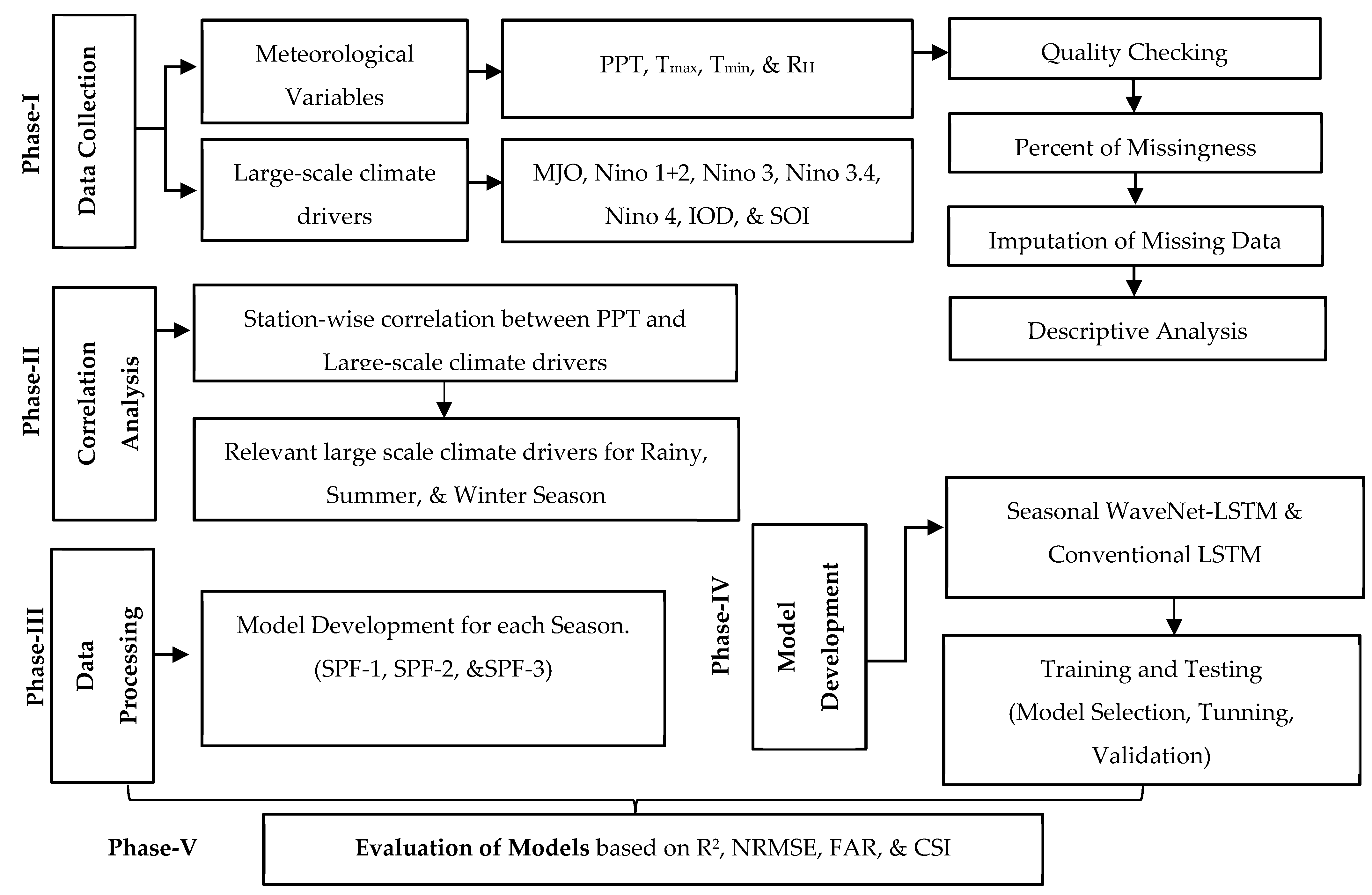
2. Materials and Methods

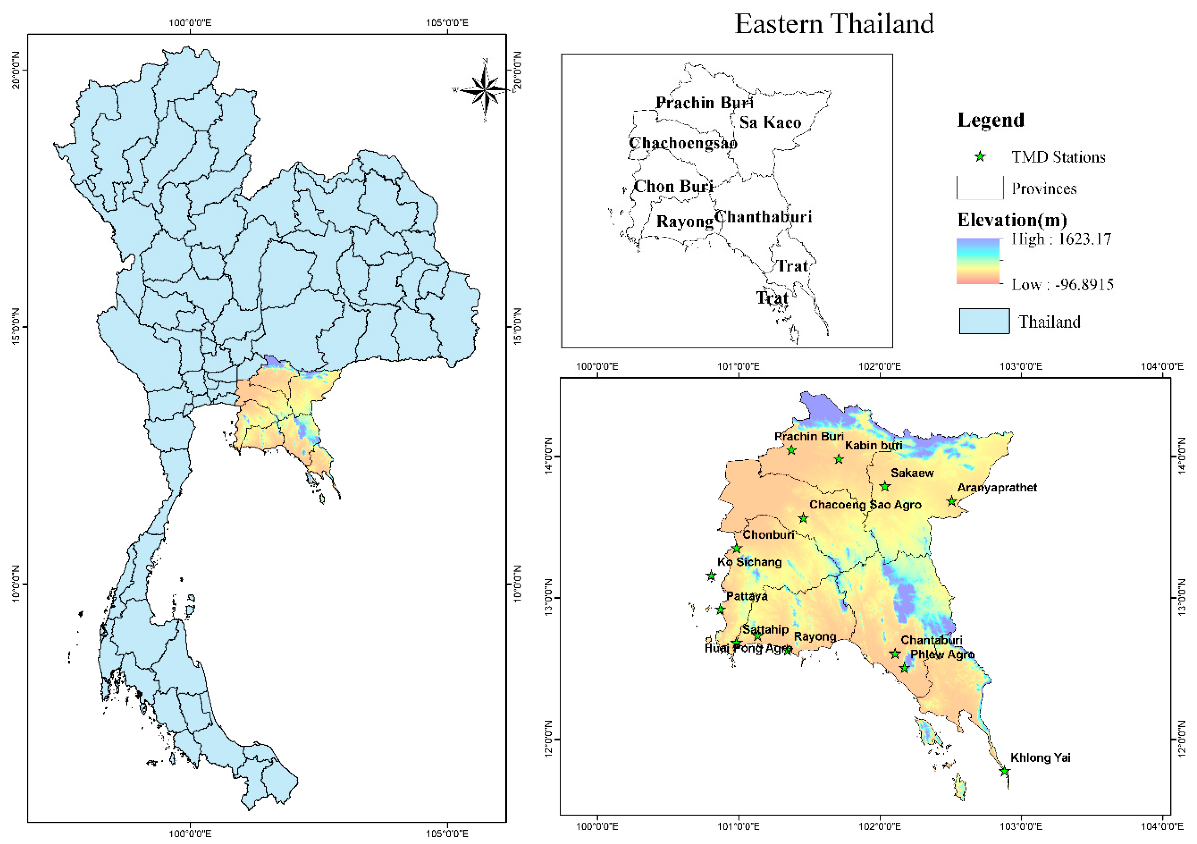
This section incorporates relevant large-scale climate drivers, such as the IOD, ENSO, SOI, MJO, and MEI, alongside meteorological variables to address the study’s objectives. A comprehensive correlation analysis of these climate drivers with seasonal precipitation in Eastern Thailand informs the selection of large-scale climate drivers for building prediction models. For SPF, this study integrates LSTM networks with RNNs, and WT is utilized to decompose and enhance the forecasting capabilities of the SPF model. A Seasonal WaveNet-LSTM model is built with prediction powers that are comparable to those of traditional LSTM. Figure 1 presents the overall methods employed to achieve these objectives.

2.1. Study Area

Thailand is located between latitudes 5°37′ to 20°27′ N and longitudes 97°22′ to 105°37′ E [33], as shown in Figure 2. The country experiences three seasons. The rainy season lasts from mid-May to mid-October, driven by the southwest monsoon that brings warm, humid air from the Indian Ocean, which results in heavy rainfall. July and August are the wettest months. The winter season extends from mid-October to mid-February and is marked by the northeast monsoon, which brings cold, dry air from China to Northern Thailand. The summer season, from mid-February to mid-May, is a transitional period from the northeast to the southwest monsoon-caused higher temperatures, with April being the hottest month [48,49]. Eastern Thailand, located between the Sankamphaeng Range and the Gulf of Thailand, features the Chanthaburi Range and small river basins draining into the Gulf [50,51]. This region covers 34,381 km2 across seven provinces: Chachoengsao, Chanthaburi, Chonburi, Prachinburi, Rayong, Sa Kaeo, and Trat, which account for 6.70% of Thailand’s total land area. In 2010, land use was approximately 62.49% agricultural, 22.92% forest, 6.84% urban, 2.46% water bodies, and 5.29% miscellaneous [52]. The Eastern Sea coast, a critical industrial zone, faces increasing water demand due to population growth and economic development. Rainfall variability significantly impacts agriculture and industry, as determined during the severe drought of 2005 when water conflicts forced the industrial sector to transport water from nearby regions [48,53].

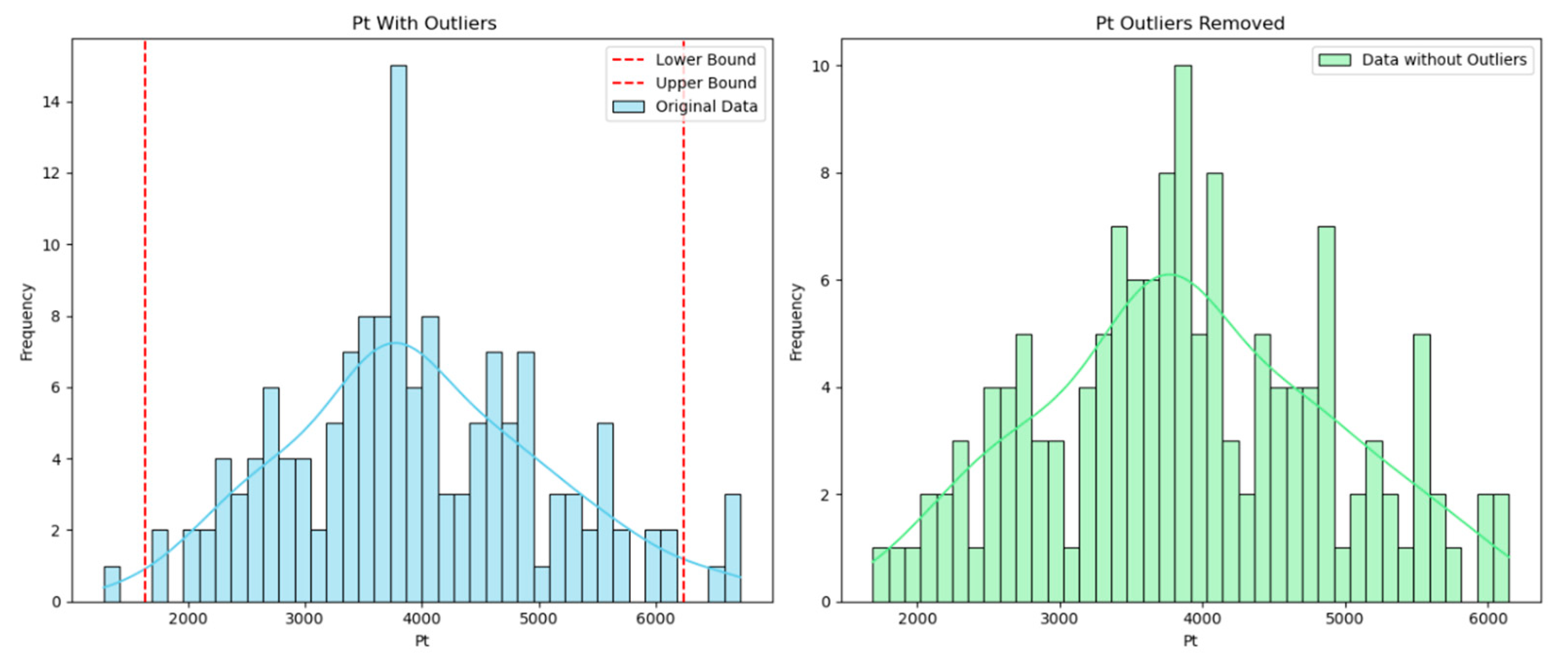
2.2. Data Collection and Quality Checking

This study analyzed a 30-year dataset (1993–2022) from 14 Thai Meteorological Department (TMD) stations, including daily precipitation, temperature, and relative humidity. Missing values were handled using the LSTM-RNN imputation approach from Wangwongchai (2023) [54]. Accurate checks addressed observational errors, excluding stations with over ten consecutive missing days or significant outliers [55]. The Grubbs and Beck (1972) technique identified significant deviations, ensuring data integrity through detailed quality assessment, removing extreme values, and interpolating missing data [56]. These procedures helped this study with quality checking and maintaining the accuracy and reliability of the meteorological indices used in the analysis, ensuring robust and dependable results.

Table 1. Descriptive daily precipitation statistics for selected TMD stations by season (1993–2022).

Stations	Summer (Mid-Feb to Mid-May)						Rainy (Mid-May to Mid-Oct)						Winter (Mid-Oct to Mid-Feb)
	Mean	Min	Max	SD	CV	Skew	Mean	Min	Max	SD	CV	Skew	Mean	Min	Max	SD	CV	Skew
Chacoeng Sao Agro	3.80	0	101.60	9.55	2.52	4.11	6.33	0	130.50	11.96	1.89	3.40	1.16	0	88.90	4.64	3.99	10.06
Chonburi	2.84	0	105.40	8.76	3.08	5.21	6.16	0	163.40	13.14	2.13	3.95	0.99	0	74.00	4.00	4.02	7.48
Ko Sichang	2.40	0	105.20	8.06	3.36	5.51	5.57	0	184.00	12.50	2.25	4.25	1.03	0	95.70	5.10	4.94	9.83
Pattaya	2.26	0	113.30	7.73	3.42	5.37	5.20	0	194.20	12.75	2.45	5.07	1.14	0	64.50	4.91	4.32	7.12
Sattahip	3.16	0	156.20	10.33	3.27	6.11	6.23	0	244.40	14.54	2.33	5.61	1.57	0	80.10	5.60	3.57	6.53
Rayong	3.35	0	128.40	10.70	3.19	5.20	6.50	0	193.00	14.80	2.28	4.27	1.27	0	147.50	5.76	4.52	11.36
Huai Pong Agro	3.91	0	123.00	10.98	2.81	5.01	7.05	0	183.90	14.19	2.01	3.85	1.74	0	111.30	6.29	3.63	7.15
Chantaburi	5.92	0	135.00	13.81	2.33	3.80	15.23	0	394.90	25.21	1.65	3.83	1.94	0	113.80	6.13	3.16	6.68
Phlew Agro	6.86	0	204.80	15.34	2.23	4.48	16.98	0	409.50	27.37	1.61	3.44	2.25	0	96.30	6.79	3.02	5.42
Khlong Yai	7.98	0	164.40	15.77	1.98	3.43	25.95	0	445.30	40.32	1.55	3.26	3.16	0	102.40	8.23	2.60	4.33
Laem Chabang Port	2.18	0	100.20	7.15	3.29	5.55	5.27	0	126.00	11.75	2.23	3.94	0.99	0	176.50	5.06	5.14	17.97
Prachin Buri	3.10	0	189.00	10.67	3.45	6.25	8.95	0	194.90	16.90	1.89	3.44	0.44	0	72.90	3.39	7.73	13.96
Kabin Buri	2.97	0	125.40	9.54	3.21	5.48	7.75	0	159.90	14.21	1.83	3.14	0.58	0	99.70	4.23	7.24	14.12
Sakaew	2.06	0	119.90	7.17	3.49	5.99	5.41	0	181.50	12.13	2.24	4.54	0.49	0	70.40	3.17	6.45	13.02

presents comprehensive descriptive statistics of daily precipitation for three seasons at TMD stations.

In summer, rainfall varies significantly. For example, Chachoeng Sao Agro station has a mean daily precipitation of 3.80 mm, a maximum of 101.60 mm, and a standard deviation (SD) of 9.55 mm, indicating high variability. A skewness of 4.11 suggests occasional extreme rainfall events. Similarly, Chonburi has a mean of 2.84 mm and a skewness of 5.21, highlighting a skewed distribution with extreme occurrences. During the rainy season, precipitation increases. Chantaburi, for example, shows a mean daily precipitation of 15.23 mm, a maximum of 394.90 mm, and a skewness of 1.94, indicating heavy rain. Khlong Yai experiences even higher rainfall, with a mean of 25.95 mm, a maximum of 445.30 mm, and a skewness of 3.43, showing a propensity for extreme rainfall. In winter, precipitation is significantly lower. Chachoeng Sao Agro records a mean daily precipitation of 1.16 mm and a maximum of 88.9 mm, with a skewness of 10.06, reflecting mostly dry days with occasional heavy rain. Rayong and Khlong Yai report mean daily precipitation of 1.27 mm and 3.16 mm, respectively, with high skewness values, indicating irregular but significant rainfall. The statistics illustrate distinct seasonal variations, with the rainy season characterized by heavier, more variable rainfall and the summer and winter seasons by lower, but occasionally extreme, precipitation—

Table 2. Large-scale climate drivers with spatial domain, technical description, and data source.

Large-Scale Climate Drivers	Spatial Domain	Technical Description	Data Source
NIÑO3.4	(5 S–5 N,170 W–120 W)	The ENSO phenomenon is recognized via two leading indicators: (a) the SOI, which measures anomalies in sea level pressure between Darwin and Tahiti, and (b) SST anomalies, assessed using the Niño indices: Niño3, Niño4, and Niño3.4 in the equatorial Pacific Ocean [8].	https://www.cpc.ncep.noaa.gov/data/indices/sstoi.indices (accessed on 12 February 2024)
NIÑO3	(5 N–5 S, 150 W–90 W)
NIÑO4	(5 N–5 S, 160 E–150 W)
NIÑO1+2	(0–10 S, 90 W–80 W)
IOD	(50° E–70° E and 10° S–10° N) (90° E–110° E and 10° S–0° S)	The IOD is measured using the DMI, which represents the difference in average sea surface temperature anomalies between the tropical western Indian Ocean (50° E–70° E, 10° S–10° N) and the tropical Eastern Indian Ocean (90° E–110° E, 10° S–0° S).	https://psl.noaa.gov/gcos_wgsp/Timeseries/Data/dmi.had.long.data (accessed on 12 February 2024)
SOI	---	The SOI reflects anomalies in sea level pressures between Darwin and Tahiti [8].	https://climexp.knmi.nl (accessed on 12 February 2024)
MJO	---	The MJO is an eastward-moving cloud and rainfall pattern that takes 30 to 60 days to return to its starting point. Unlike ENSO, the MJO’s characteristics vary weekly, offering intra-seasonal tropical climate variability. Multiple MJO events can occur in a single season [57].	https://iridl.ldeo.columbia.edu/SOURCES/.BoM/.MJO/.RMM/.RMM1/ (accessed on 12 February 2024)
MEI	(30° S–30° N, 100° E–70° W)	The MEI is a time series from an EOF analysis of sea level pressure, sea surface temperature, wind components, and OLR in the tropical Pacific. It accounts for ENSO seasonality across overlapping two-month periods to minimize intra-seasonal variability.	https://psl.noaa.gov/enso/mei/ (accessed on 12 February 2024)

details large-scale climate drivers, including sources and technical descriptions.

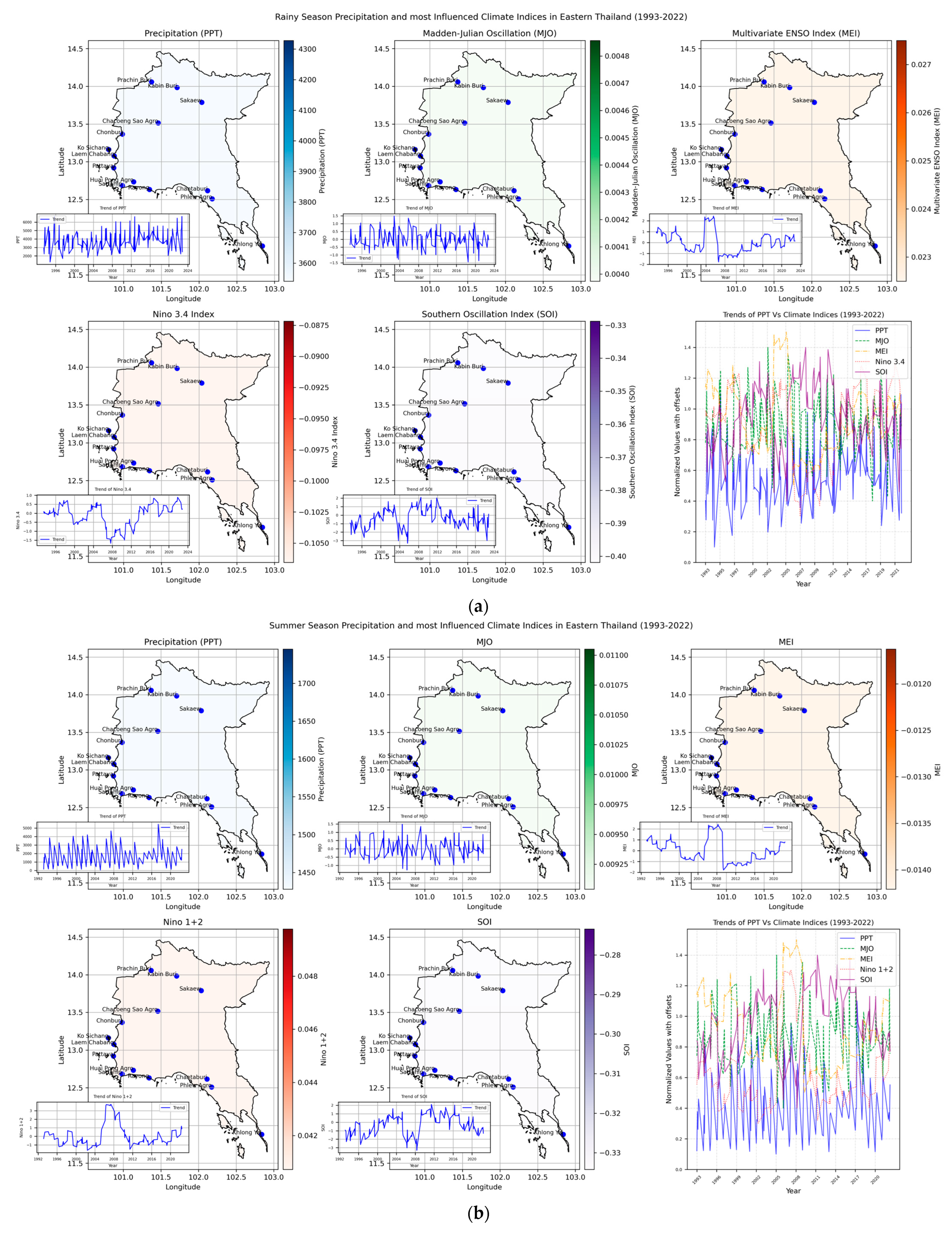
2.3. Correlation Analysis Between Seasonal Precipitation and Large-Scale Climate Drivers

This study employed Pearson’s correlation (r) to examine the influence of climate drivers on SPF. Pearson’s correlation is a statistical metric that evaluates the linear relationship between two continuous variables. The correlation coefficient ranges from −1.00 to +1.00, where −1.00 denotes a perfect negative correlation, +1.00 signifies a perfect positive correlation, and 0.00 indicates no relationship between the variables [58].

$$Pearson’s Correlation (r)={\displaystyle \frac{n(\sum xy)-(\sum \mathrm{x}\left)\right(\sum \mathrm{y})}{\sqrt{[n\sum {\mathrm{x}}^2-(\sum {\mathrm{x}}^2\left)\right][n\sum {\mathrm{y}}^2-\left(\sum {\mathrm{y}}^2\right)}}}$$

(1)

The correlation analysis of precipitation during the rainy season with large-scale climate drivers, as illustrated in Figure 3a, reveals a complex interplay between regional precipitation and climate drivers. For example, Chachoengsao Agro exhibits a positive correlation of 0.23 with the MJO, indicating that increased MJO activity corresponds with higher precipitation. A negative correlation of −0.10 with the MEI indicates reduced precipitation during El Niño conditions. At Ko Sichang, a negative correlation of −0.25 with MEI further emphasizes the diminished precipitation experienced during El Niño events. In addition, indices associated with La Niña, such as the SOI, often positively correlate with precipitation.

For example, a strong positive correlation of 0.28 with the SOI at Sattahip highlights increased precipitation during La Niña events. These findings emphasize the impact of large-scale climate phenomena on regional weather patterns. The consistent positive correlation between MJO and precipitation observed across various stations, including Chachoengsao Agro (0.23), Ko Sichang (0.25), and Pattaya (0.22), reinforces the MJO’s role in augmenting rainfall during active phases. Based on this comprehensive correlation analysis, climate drivers such as MEI, Niño 3.4, SOI, and MJO have been identified as critical indicators with a high correlation to precipitation during the rainy season. Their relevance makes them suitable for inclusion in SPF model development.

The correlation analysis for the summer season reveals the broader climate patterns that impact regional weather, as shown in Figure 3b. At Chachoengsao Agro, a strong negative correlation with the MJO (−0.26) suggests a decrease in regional precipitation during heightened MJO activity, indicating that the MJO can suppress precipitation in the area during its active phases. Similarly, at Chonburi, the analysis reveals significant negative relationships with MJO (−0.33) and MEI (−0.26), suggesting that MJO activity and El Niño conditions are associated with reduced precipitation in this region. These combined influences highlight the compounded effect of these climate indices on regional weather. At Ko Sichang, a negative correlation between MJO activity (−0.18) and MEI (−0.17) further emphasizes the impact of both MJO and El Niño events on regional precipitation during the summer. The consistent negative correlations observed across multiple stations emphasize the complex interaction between large-scale climate phenomena and regional weather patterns. After conducting a comprehensive correlation analysis of climatic indices such as Niño 1+2, MEI, SOI, and MJO, these climate drivers were selected due to their significant association with precipitation patterns during the rainy season. Their strong correlation provides valuable insights into the variability and distribution of rainfall, making them essential for refining the accuracy of the SPF model.

The correlation analysis for the winter season provides a detailed examination of the intricate relationship (Figure 3c). At Chachoengsao Agro, a positive correlation with Niño 3.4 (0.16) suggests that El Niño conditions, characterized by warmer sea surface temperatures in the Central and Eastern Tropical Pacific, are associated with increased regional precipitation during the winter season. Similarly, at Chonburi, positive correlations with Niño 3 (0.18) and Niño 3.4 (0.27) highlight the relationship between these indices and augmented regional precipitation. These patterns imply that El Niño events significantly impact regional weather. At Ko Sichang, the positive correlations between Niño 3 (0.11) and Niño 3.4 (0.15) further support the link between warmer sea surface temperatures in these regions and increased precipitation during the winter season.

Additionally, negative correlations with the SOI at multiple stations, such as Chonburi (−0.25) and Huai Pong Agro (−0.20), indicate that a decrease in SOI, signifying El Niño conditions, corresponds with increased precipitation. It suggests a significant interplay between El Niño dynamics and local weather systems. A decrease in SOI correlates with warmer sea surface temperatures in the Eastern Tropical Pacific, contributing to El Niño conditions and influencing regional precipitation patterns. These findings demonstrate that seasonal climate drivers, such as the MJO and El Niño, significantly influence regional weather during the winter months. Following a comprehensive correlation analysis of Niño 3, Niño 3.4, Niño 4, and SOI, these climatic indices were selected due to their strong association with precipitation patterns during the winter season.

To gain deeper insights into the complex relationship between selected large-scale climate drivers and seasonal PPT provides a comprehensive view of how these indices influence PPT patterns. For the rainy season, the relationship between the MJO, MEI, Niño 3.4, and SOI with precipitation is shown in Figure 4a. The MJO’s positive phases are correlated with increased precipitation, like the summer season, indicating its significant impact on rainy season rainfall. The MEI values, when positive (El Niño), tend to show decreased precipitation, whereas negative values (La Niña) exhibit varied impacts on rainfall [59]. The Niño 3.4 index, with its positive values, correlates with lower precipitation during the rainy season, indicating that La Nina events cause more rainfall. The SOI also follows this pattern, where negative values (El Niño) are associated with decreased precipitation, and positive values (La Niña) align with higher precipitation levels [60]. Figure 4b shows the behavior of the MJO, MEI, Niño 1+2 index, and SOI with summer precipitation. The MJO, characterized by its varying positive and negative phases, exhibits significant variability [23]. Positive MJO phases, marked by red dots, often correspond to increased precipitation, suggesting a potential relation between the MJO’s positive phases and higher summer rainfall.

Similarly, the MEI, which oscillates between El Niño and La Niña phases, shows a trend where positive MEI values are associated with decreased precipitation, implying that El Niño conditions might enhance summer precipitation. The Niño 1+2 follows a similar pattern, with positive values generally aligning with lower precipitation levels. This consistent pattern across different indices highlights the significant role of El Niño in boosting summer precipitation. During the winter season, the relationship between various Niño indices (Niño 3, Niño 3.4, and Niño 4) and the SOI with precipitation is explored in Figure 4c. The positive values of the Niño 3 index, indicating El Niño conditions, are generally associated with higher winter precipitation. This trend is consistent across the Niño 3.4 and Niño 4 indices, where positive values align with increased precipitation, reinforcing the strong influence of El Niño. The SOI during winter also shows a similar pattern, where El Niño corresponds to higher precipitation, and La Niña correlates with lower precipitation. This consistency suggests that El Niño significantly enhances winter rainfall, while La Niña tends to reduce it. The analysis reveals a consistent pattern where El Niño conditions (indicated by positive values in Niño indices and negative values in SOI) generally lead to increased precipitation across all seasons. It is evident in the summer and winter seasons, where the impact of El Niño is more pronounced.

Conversely, La Niña conditions (negative values in Niño indices and positive values in SOI) correspond to lower precipitation, although the effect is more variable during the rainy season. The MJO also plays a crucial role during the summer and rainy seasons, with its positive phases correlating with higher precipitation. These findings emphasize the significant influence of large-scale climate drivers like ENSO and MJO on seasonal precipitation patterns, providing valuable insights for understanding climate variability and predicting seasonal weather impacts.

2.4. Model Development

The input models are designed to capture the intricate interactions of these variables across the summer, rainy, and winter seasons.

Table 3. Models based on relevant features were selected based on correlation analysis between large-scale climate drivers and seasonal precipitation.

Model/ Target	Features
	Summer	Rainy	Winter
SPF-1/PPT	Niño 1+2FMAM, MJOFMAM, MEIFMAM, SOIFMAM	MJOMJJASO, MEIMJJASO, Niño 3.4MJJASO, SOIMJJASO	Niño 3ONDJF, Niño 3.4ONDJF, Niño 4ONDJF, SOIONDJF
SPF-2/PPT	TminFMAM, TmaxFMAM, RHFMAM, Niño 1+2FMAM, MEIFMAM, MJOFMAM, SOIFMAM	TminMJJASO, TmaxMJJASO, RHMJJASO, MJOMJJASO, MEIMJJASO, Niño 3.4MJJASO, SOIMJJASO	TminONDJF, TmaxONDJF, RHONDJF, Niño 3ONDJF, Niño 3.4ONDJF, Niño 4ONDJF, SOIONDJF
SPF-3/PPT	P(t − 1) FMAM, P(t − 2) FMAM, P(t − 3) FMAM, P(t − 4) FMAM and P(t − 5) FMAM	P(t − 1) MJJASO, P(t − 2) MJJASO, P(t − 3) MJJASO, P(t − 4) MJJASO and P(t − 5) MJJASO	P(t − 1) ONDJF, P(t − 2) ONDJF, P(t − 3) ONDJF, P(t − 4) ONDJF and P(t − 5) ONDJF

presents the models selected based on the correlation analysis between large-scale climate drivers and seasonal precipitation. Model SPF-1 integrates PPT with key ENSO indices, such as Niño 1+2, Niño 3, Niño 3.4, and Niño 4, along with the MEI and SOI for the summer (mid-February to mid-May) and winter (mid-October to mid-Feb) seasons. During the rainy season (mid-May to mid-October), this model also incorporates the MJO, Niño 1+2, and Niño 3.4, along with SOI. This configuration reflects the significant role of ENSO and MJO in influencing seasonal precipitation, as previously established by correlation analysis. Model SPF-2 expands the feature set to include T_min and T_max, R_H, and additional ENSO indices. This broader approach considers other climatic factors that can impact precipitation patterns. SPF-3 focuses on accounting for the temporal dependencies of precipitation by utilizing current and lagged precipitation values (P(t), P(t − 1), P(t − 2), P(t − 3), P(t − 4), and P(t − 5)). This model emphasizes the persistence and autocorrelation in precipitation data, which is crucial for accurate SPF across all seasons. These models integrate key climatic drivers and historical precipitation data to comprehensively understand the influence of ENSO indices, MJO, T_max, T_min, R_H, and temporal patterns on seasonal precipitation variability and prediction.

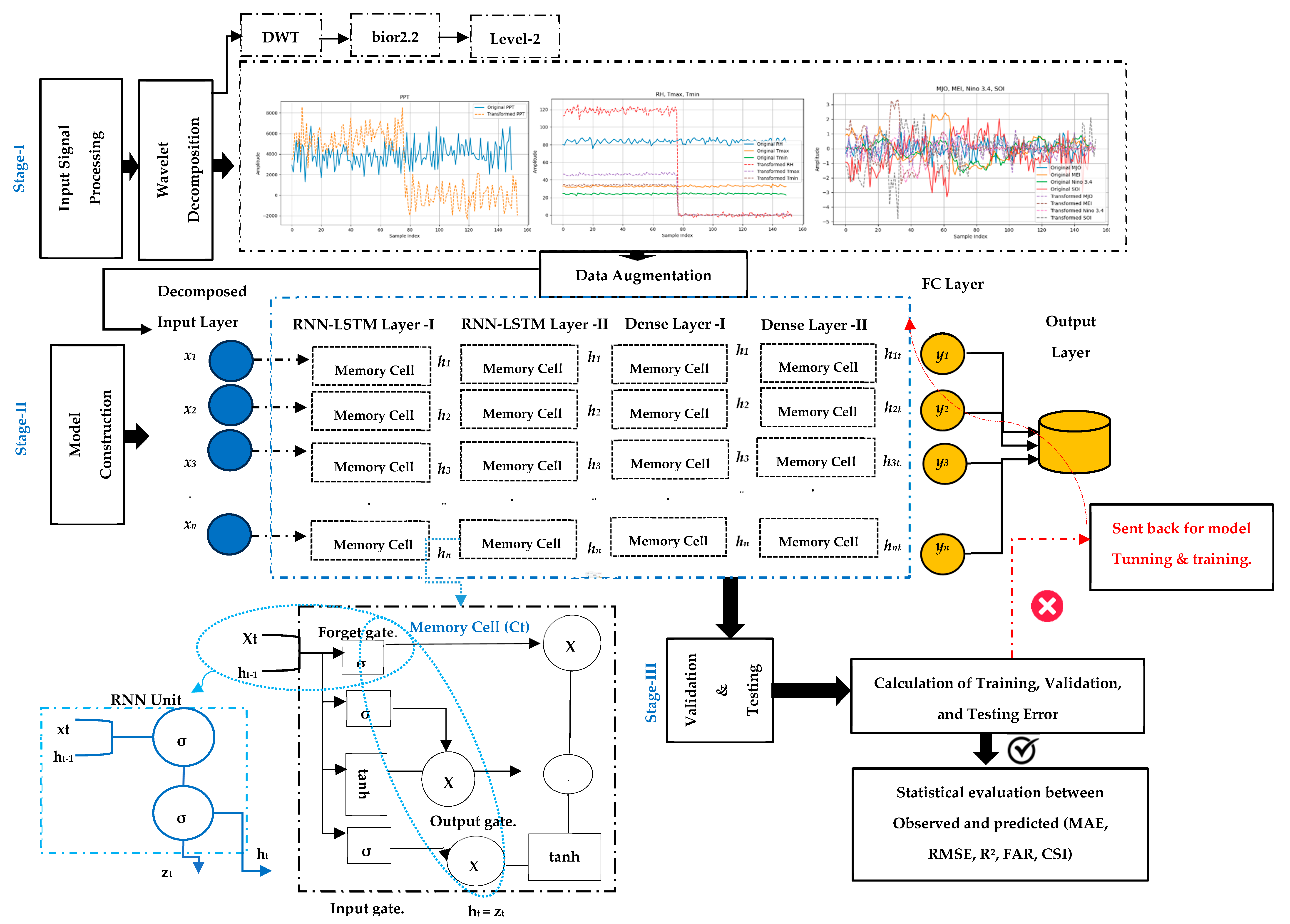
2.5. Seasonal WaveNet-LSTM

This study presents a novel “Seasonal WaveNet-LSTM” model, a hybrid approach combining wavelet transformation (WT) and RNN with LSTM networks to address the limitations of traditional RNNs [61] in SPF [45]. The Seasonal WaveNet-LSTM model’s dependability is heavily dependent on data preprocessing, which includes handling missing data and detecting outliers. Missing data were addressed using the imputation approach suggested by Wangwongchai (2023), which takes into account temporal dependencies and the consistency of climate variables [54]. It ensures that missing data and outliers do not add bias to the temporal patterns required for accurate wavelet decomposition and RNN-LSTM training. Outliers were discovered and treated based on their possible impact on the overall data distribution, with extreme values distorting WT results, as shown in Figure 5.

The seasonal WaveNet-LSTM model is built in three stages: wavelet decomposition, model construction, training, validation, and testing, as shown in Figure 6. In the first stage, WT decomposes the precipitation signal into wavelets, offering time–frequency representations in the time domain [62]. WT encompasses both the Continuous Wavelet Transform (CWT) and the Discrete Wavelet Transform (DWT). CWT involves calculating the product of the signal and the wavelet function, providing a continuous and thorough time–frequency representation. While CWT offers detailed analysis, its wavelet coefficients can be redundant [11]. DWT addresses redundancy by using discretely sampled wavelets, which reduces the amount of data required for processing [47]. It made a powerful tool for analyzing signal patterns in both time and frequency domains [63]. DWT effectively filters out noise and captures essential timescale information in complex signals, like non-linear and non-stationary precipitation rates [64,65]. DWT was incorporated in this study based on the nature of the time series input dataset. The model systematically applied various mother wavelet functions, ψ(t), to identify the most suitable wavelet across all decomposition levels. Subsequently, the most appropriate wavelet function (bior2.2) and decomposition level were selected based on their performance in representing the data effectively. The chosen mother wavelet function ψ(t) (bior2.2) wavelet at level 2 functions as a sequence of configurable moving windows for local temporal pattern identification [45,66].

In the second stage, the LSTM model contains an internal state and three important gates within each LSTM cell: forget, input, and output [67]. These gates regulate the flow of information at each time step t, using inputs from x_t and the previous hidden state h_t−1. The forget gate employs a sigmoid function to determine whether to retain or discard information from the previous time step. The input gate combines sigmoid and tanh activation layers to update the cell state. The output gate establishes the hidden state value for the next time step, influencing the network’s predicted outcome. The architecture consists of two LSTM layers, each with 50 hidden nodes using a tanh activation function for cell state updates. The input gate uses a sigmoid activation function to regulate the flow of current information into the cell state, and the forget gate, also employing a sigmoid activation function, oversees the retention of past cell states. The cell candidate employs the tanh activation function to introduce potential new values, which are combined with the previous cell state via the output gate’s sigmoid activation function. The overall cell state and hidden state are derived from these mechanisms.

The model integrates large-scale climate drivers and P_t, T_max, T_min, and R_H time series datasets. The model is trained using the Adam optimizer with a learning rate of 0.001 over 500 epochs, ensuring robust training while minimizing overfitting. The configuration is enhanced using orthogonal initialization for input weights and bi-orthogonal initialization for recurrent weights, contributing to efficient training and model stability. Performance metrics such as R², NRMSE, FAR, and CSI validate the model’s accuracy, particularly in capturing long-term dependencies in time series data. Despite its strengths, the model’s complexity and sensitivity to wavelet decomposition levels and types of present challenges in hyperparameter tuning and computational resources.

Table 4. Seasonal WaveNet-LSTM model’s parameters and optimal configurations.

Feature Name	Optimal Configuration	Mathematical Description
Features	Large-scale climate drivers, Tmax, Tmin, RH, and Lagged PPT	$Input Gate=\sigma (W_i\left[x_t,h_{t-1}\right]+b_i)$ (2) $Forget Gate=\sigma (W_f\left[x_t,h_{t-1}\right]+b_f)$ (3) $Cell candidate=tanh\left(W_c\left[x_t,h_{t-1}\right]+b_c\right)$ (4) $Cell State {=C}_t=f_t\times \left[C_{t-1}+i_t\right]\times {\overline{C}}_t$ (5) $Output Gate=(W_o\left[X_t,h_{t-1}\right]+b_o)$ (6) $Hidden State=o_t\times Sigmoid \left(C_t\right)$ (7) The weight matrices and bias for the input, forget, cell candidate, and output gates are denoted by “W” and “b”, respectively. “Xt” represents the memory cell’s input, “ht−1” represents the hidden state at the previous time step “t − 1”, and “Ct−1” and “Ct” represent the cell states at the previous time step “t − 1” and the current time step “t”, respectively.
Responses	Precipitation in mm
No. of hidden nodes	50 in each LSTM layer
Optimizer	Adam
Learning rate	0.001
Epoch	500
Wavelet decomposition	bior2.2 at level 2
LSTM Layer Configuration 1	LSTM (50, activation = ‘tanh’, return sequences = True)
LSTM Layer Configuration 2	LSTM (50, activation = ‘tanh’)
Dense Layer Configuration 1	Dense (20, activation = ‘tanh’)
Dense Layer Configuration 2	Dense (20, activation = ‘sigmoid’)
Output Layer	Dense (1, activation = ‘sigmoid’)
Bias Initialization	Unit-forget-gate bias initialization
Function (gates)	Sigmoid activation function
Function (input weights)	Orthogonal initialization for input weights
Function (recurrent weights)	Bi-orthogonal initialization for recurrent weights
Performance metrics	R2, NRMSE, FAR, CSI

summarizes the optimal configurations and mathematical descriptions of the Seasonal WaveNet-LSTM model. With greater precision, this approach captures the underlying patterns and temporal dependencies in highly non-linear and non-stationary signals, such as precipitation rates. Traditional LSTM models, while capable of learning long-term dependencies, struggle with high-frequency noise and fail to capture complex signal dynamics. The Seasonal WaveNet-LSTM model addresses these limitations by incorporating wavelet-transformed inputs, improving forecasting accuracy and robustness.

The Seasonal WaveNet-LSTM model used WT to improve forecast accuracy by breaking down input signals into constituent frequencies. This decomposition stage enables the model to handle both high- and low-frequency components more successfully than typical LSTM designs, which can struggle with complex seasonal patterns and high-frequency noise in the data. Using wavelet-transformed inputs, the model captured strong temporal dependencies across several scales, which is critical for forecasting highly non-linear and non-stationary signals such as precipitation rates. The DWT, notably the bior2.2 wavelet at level 2, provides an efficient time–frequency representation that eliminates redundancy in data while also successfully filtering out noise. This filtering enables the RNN and LSTM layers to focus on essential patterns without being muddled by noise, boosting model robustness and forecast accuracy. The hierarchical decomposition using wavelets provides a noticeable benefit in expressing seasonal fluctuations, resulting in a more accurate prediction of precipitation over time.

Limitations of Seasonal WaveNet-LSTM

The Seasonal WaveNet-LSTM model, while effective, introduces considerable computational challenges and trade-offs. Wavelet decomposition, while enhancing temporal pattern recognition, imposes significant memory and processing demands. This complexity intensifies with larger datasets, necessitating substantial computational resources for model training. Achieving optimal parameter configurations requires extensive experimentation, which is computationally intensive. Balancing model accuracy with computational efficiency presents a further trade-off, while deeper decomposition level (i.e., level 2) improved temporal pattern capture.

While this model is designed for Eastern Thailand, where monsoonal dynamics and regional climate drivers heavily influence seasonal precipitation patterns, it has the potential for use in other regions. However, adaptation may be required for places with varying rainfall dynamics, such as those affected by localized climate patterns or reduced seasonality. To account for changes in places where large-scale climatic drivers have less influence, the model may need to be recalibrated, notably in the weighting and selection of input features. Furthermore, rainfall dynamics in other regions may have distinct frequency and amplitude characteristics, influencing the applicability of the chosen wavelet (bior2.2) or the depth of decomposition. For places with diverse seasonal cycles, it may be advantageous to investigate alternate wavelet functions or decomposition procedures to ensure that the model reflects the relevant temporal dependencies and signal properties unique to that climate regime

2.6. Evaluation Criteria

For the training and testing dataset, the SPF is validated against observed values, including Normalized Root Mean Square Error (NRMSE) and Coefficient of Determination (R²), False Alarm Ratio (FAR), and Critical Success Index (CSI), like precision and recall in ML [68].

$$Normalized Root Mean Square Error=NRMSE={\displaystyle \frac{\frac{\sqrt{\sum _{i=1}^N{(Pobs-Ppre)}^2}}{N}}{\sigma }}$$

(8)

$$Coefficient Determination=R^{2 }={\displaystyle \frac{n\left(\Sigma Pobs\ast y\right)-\left(\Sigma Pobs\right)\left(\Sigma Ppre\right)}{\sqrt{n\left[\Sigma Pobs2-\left(\Sigma Pobs2\right)\right]\left[\Sigma Ppre2-\left(\Sigma Ppre2\right)\right]}}}$$

(9)

$$False Alarm Ratio=FAR={\displaystyle \frac{FA}{FA+Hits }}$$

(10)

$$Critial Success Index=CSI={\displaystyle \frac{Hits}{Hits+FA+Misses}}$$

(11)

P_obs, P_pre, and P_mean, are observed and predicted as the precipitation mean, respectively. The R² varies between 0 to 1. It is widely used to assess hydrological approaches [69]. NRMSE is a crucial performance statistic that quantifies the accuracy of predictive models by calculating the average percentage of errors in projected values quantities compared to observed values [70]. A Hit occurs when the predicted rainfall matches the observed rainfall. An FA (False Alarm) happens when the forecasted category is higher than the actual observed category, and a Miss occurs when the predicted category is lower than the observed one [71]. FAR and CSI scores range from 0 to 1, with lower FAR and higher POD and CSI values being better [72,73].

3. Results

The SPF results of the Seasonal WaveNet-LSTM models for the rainy season reveal critical insights into the model’s performance and the importance of various inputs. For rainy season precipitation prediction, the SPF-1 model, which uses the SOI, Niño 3.4, MEI, and MJO indices as inputs, the variable importance scores show that Niño 3.4 and MJO are the most influential predictors, with 27.8% and 25.4%, respectively (Figure 7a). SOI and MEI have slightly lower importance of 24.0% and 22.8%. This model achieved an R² of 0.55, indicating moderate explanatory power. The NRMSE of 19.98% reflects reasonable accuracy in predictions, while the FAR of 0.29 and CSI of 0.50 suggest false alarms and event detection challenges. In contrast, the SPF-2 model, which incorporates a broader range of meteorological variables and large-scale drivers (T_max, T_min, RH, SOI, Niño 3.4, MEI, and MJO), exhibits different dynamics in variable importance. The highest importance is assigned to T_min and T_max, with 18.6% and 15.4%, respectively, while SOI, Niño 3.4, MEI, MJO, and R_H have comparable importance between 11.7 and 15.0%. The performance metrics for SPF-2 are notably superior, with an R² of 0.89 and a reduced NRMSE of 10.25%, indicating higher accuracy and better model fit. This model has a lower FAR of 0.14 and a higher CSI of 0.86.

The SPF-3 model has high R² and low NRMSEs, especially during the rainy season (R² = 0.91, NRMSE = 8.86%), indicating great predictive accuracy. The variable importance scores show that (P-4) is the most influential predictor, with an importance of 26.5%, while the influence of previous values decreases progressively. Despite the high accuracy, the model is FAR, the highest at 0.03, and the CSI, the lowest at 0.97, suggesting significant false alarms and correct event detection. However, the model’s reliance on lagged precipitation data (P-1 to P-5) raises issues about overfitting, especially considering that significant autocorrelation in precipitation patterns might cause models to fit noise rather than capture underlying dynamics. However, using historical precipitation data increases near-term prediction accuracy. It impairs model robustness across a wide range of environmental variables, thus restricting generalization.

The results from the summer SPF using the Seasonal WaveNet-LSTM model provide insights into the performance and importance of input variables (Figure 7b). For SPF-1, which includes MJO, MEI, SOI, and Niño 1.2, the variable importance scores indicate that Niño 1.2 is the most influential predictor with 29.6%, followed by MEI (24.7%), SOI (23.4%), and MJO (22.4%). The model achieves a high R² of 0.87, suggesting a strong correlation between the predicted and actual values, and it has the lowest NRMSE at 12.01%, indicating a relatively low error rate. Additionally, SPF-1 exhibits a low FAR of 0.09 and a high CSI of 0.83, underscoring its robustness and reliability in predicting summer precipitation. In contrast, SPF-2 incorporates temperature variables (T_max, T_min, R_H) and the same climatic indices as SPF-1. Here, the highest importance is assigned to SOI (16.1%), while the temperature variables (T_max and T_min) and other climatic indices have lower importance scores ranging from 14.5% to 12.4%. Although SPF-2’s R² of 0.81 is slightly lower than that of SPF-1, it still indicates a good predictive performance. However, the model’s NRMSE is higher at 14.73%, suggesting a higher prediction error than SPF-1. Additionally, SPF-2’s FAR is slightly increased to 0.11, and its CSI is reduced to 0.67, indicating a moderate decline in the model’s ability to forecast summer precipitation events accurately. SPF-3, which uses previous precipitation data (P-1 to P-5) as inputs, shows the lowest variable importance scores among the three models, ranging from 18.5% to 20.8%. This model achieves an R² of 0.79, the lowest among the three, yet still signifies a good model fit. SPF-3 has the lowest NRMSE at 9.48%. Despite this, the model is FAR, the highest at 0.29, suggesting a greater tendency to miss predict precipitation events. The CSI for SPF-3 is 0.71, which is better than SPF-2 but lower than SPF-1, reflecting a balanced forecasting accuracy and reliability performance.

Figure 7c shows the results from the winter SPF. For SPF-1, which utilizes SOI, Niño 3, Niño 3.4, and Niño 4 indices, the variable importance scores indicate that Niño 4 and Niño 3.4 are the most influential predictors, with importance of 30.9% and 26.8%, respectively. SOI and Niño 3 have slightly lower importance at 22.9% and 19.4%. This model achieved an R² of 0.64, indicating a moderate level of explanatory power. The NRMSE of 19.87% reflects a reasonable level of accuracy in the predictions, while the FAR of 0.14 and CSI of 0.75 suggest that this model performs well in minimizing false alarms and correctly identifying events. For SPF-2, which incorporates T_max, T_min, R_H, SOI, Niño 3, Niño 3.4, and Niño 4, the highest importance is assigned to Niño 3.4 and Niño 4, with 16.9%. SOI, T_max, T_min, and R_H have relatively lower but comparable importance, ranging from 12.1 to 14.9%. It suggests that while the meteorological variables contribute to the model, the Niño indices remain crucial predictors. The performance metrics for SPF-2 are notably superior, with an R² of 0.79 and a reduced NRMSE of 13.69%, indicating higher accuracy and better model fit. However, the model has a higher FAR of 0.23 and a lower CSI of 0.54, suggesting that despite its higher accuracy, it struggles more with false alarms and event detection than SPF-1. SPF-3, which focuses on lagged PPT (P-1 to P-5), also demonstrates high predictive power. The model achieved an R² of 0.75 and the lowest NRMSE of 11.93%, indicating the best fit among the three models. Variable importance scores show that the most recent past precipitation value (P-1) is the most influential predictor, with an importance of 23.6%, while the influence of previous values decreases progressively. Despite the high accuracy, the model is FAR, the highest at 0.5, and the CSI, the lowest at 0.5, suggesting significant issues with false alarms and correct event detection.

The model’s performance was thoroughly evaluated during the testing period from 2017 to 2022 (30 months). For example, during the rainy season with SPF-3 input (Figure 8), a Pearson correlation coefficient (r) of 0.96 and an R² of 0.91 demonstrate a high degree of accuracy between actual and predicted precipitation. The NRMSE further reflects model precision, with most values below 0.1, indicating minimal deviation. However, higher NRMSE values (e.g., 0.18 and 0.26) indicate increased prediction errors during certain periods. The right inset illustrates feature importance, with P-4 identified as the most significant contributor. The loss curve shows convergence, with final training and validation losses of 0.0212 and 0.0150, respectively, demonstrating robust model training. Similar analyses were conducted for each season and model configuration, including SPF-1, SPF-2, and SPF-3 (Supplementary File; Figures S1–S8).

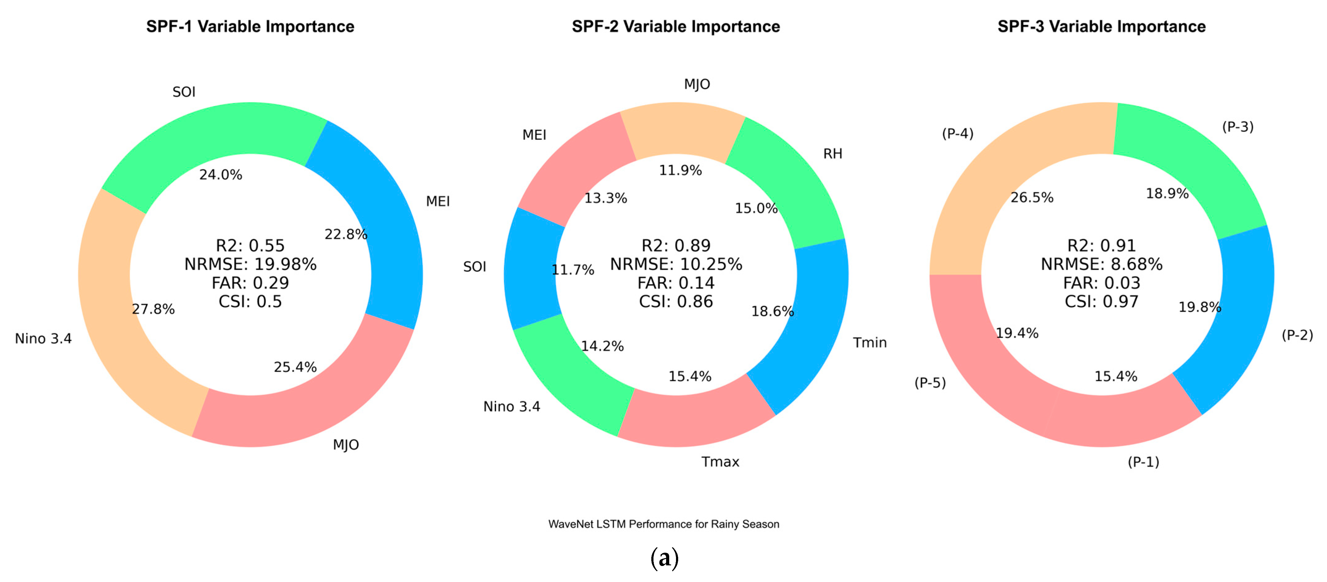
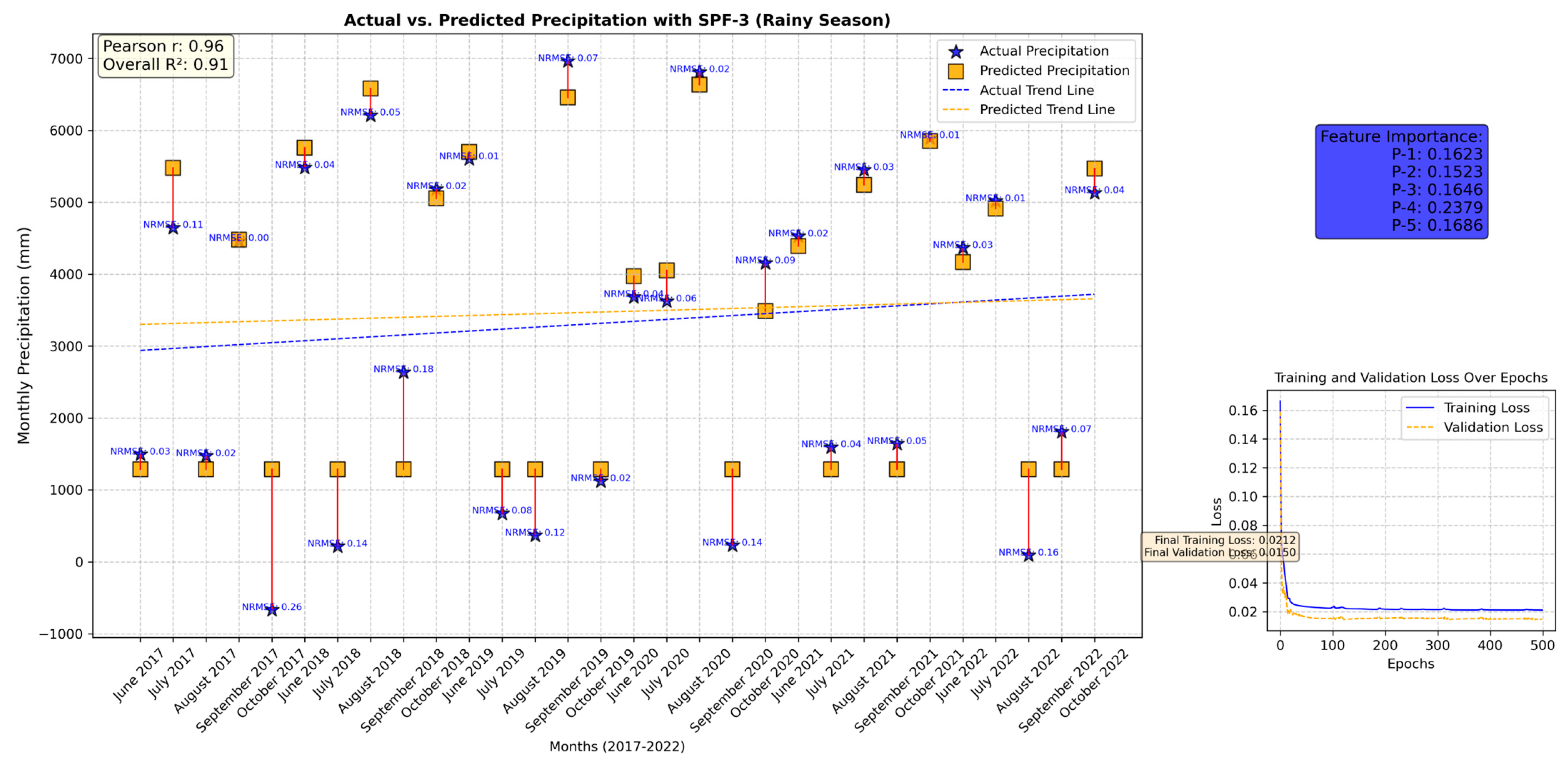
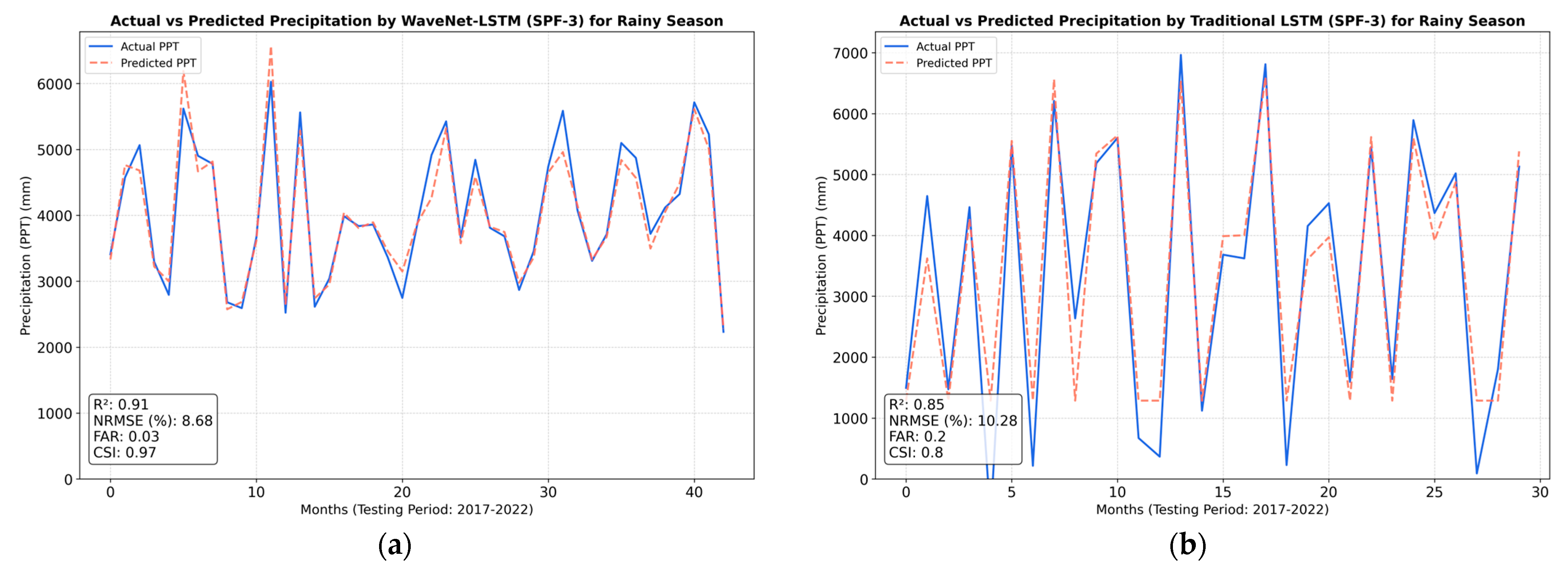
3.1. Comparative Analysis and Role of Climate Drivers in Prediction

The WaveNet LSTM model surpasses typical LSTM models in predicted accuracy and capabilities throughout all seasons, as shown in Figure 9. During the wet season, the WaveNet LSTM model (SPF-3) had an R² of 0.91, an NRMSE of 8.68%, a FAR of 0.03, and a CSI of 0.97. These measures show excellent precision and minimum error, with few false alarms and nearly perfect event detection. Compared to typical LSTM models, SPF-3 outperformed them with R² of 0.85, NRMSE of 10.28%, FAR of 0.20, and CSI of 0.80. In the summer season, the WaveNet LSTM model (SPF-1) outperformed typical LSTM models with an R² of 0.87, NRMSE of 12.01%, FAR of 0.09, and CSI of 0.83. It shows strong predictive abilities, lower error rates, and increased accuracy. Traditional LSTM models, including SPF-2, performed much worse, with an R² of 0.50, a high NRMSE of 25.37%, and a CSI of 0.67. In the winter season, the WaveNet LSTM models (SPF-2) maintained their superior performance. SPF-3 achieved an R² of 0.79, an NRMSE of 13.69%, a FAR of 0.23, and a CSI of 0.54. Traditional LSTM models significantly reduced prediction accuracy and higher error rates, while SPF-2 showed an R² of 0.20, an enhanced NRMSE of 41.46%, and a FAR of 0.80 (Figure 10).

Seasonal WaveNet LSTM models perform well in R² and CSI metrics. However, traditional LSTM models showed higher NRMSE and FAR. Despite the observed differences in NRMSE and FAR, overall technical evaluation confirmed that WaveNet LSTM models are the most effective strategy for operational SPF, with superior dependability and accuracy across all seasons.

Using large-scale climate drivers as input in ML and DL prediction models has significant implications for SPF in incorporating physical and large-scale climatic phenomena. Climate indices such as Niño 3.4, SOI, MEI, and MJO encapsulate critical information about oceanic and atmospheric processes that govern large-scale climate variability. Their integration into models allows for capturing global teleconnection patterns that impact regional precipitation, making the models helpful in predicting rainfall during events like El Niño or La Niña. For example, in the SPF-1 model for the rainy season, Niño 3.4 and MJO are identified as highly influential, contributing to over 50% of the predictive power, suggesting that these indices provide essential information for understanding precipitation variability. The primary advantage of including such indices is their ability to enhance model generalizability across diverse regions where local meteorological data may be sparse or inconsistent. By capturing the broader climate signals, models can provide more stable predictions, especially for seasonal forecasting, where global patterns dominate.

Furthermore, these indices allow the model to adapt to shifts in seasonal patterns, thus improving its robustness during extreme events. However, there are notable limitations. Large-scale indices may not adequately represent localized variability, such as microclimatic factors and terrain-induced precipitation patterns, which are crucial for precise regional predictions. For example, the SPF-1 model’s R² of 0.55 indicates that a significant portion of variability remains unexplained by large-scale indices alone. These inputs can introduce complexity into the model, as temporal resolution mismatches between climate indices and local weather data can increase noise, affecting model training and performance. Moreover, the risk of overfitting arises when numerous indices are used without sufficient regularization, leading to models that may perform well on training data but fail to generalize to unseen climatic conditions, reducing their predictive reliability.

3.2. Discussion

The Seasonal WaveNet-LSTM model revealed promising results. Including large-scale climate drivers based on correlation analysis such as the IOD, Nino indices, SOI, MJO, and MEI, alongside meteorological variables, marks a comprehensive approach to capturing the complex influences of climatic drivers on seasonal precipitation. This methodological enhancement aligns with the literature, emphasizing the importance of considering multiple climate drivers in precipitation forecasting [74,75]. The correlation analysis confirming the substantial influence of these indices on seasonal precipitation is consistent with studies indicating the pivotal role of ENSO and MJO in modulating regional weather patterns [14,23,76,77]. The SPF models developed in this study—SPF-1, SPF-2, and SPF-3—each incorporate varying combinations of climate indices and meteorological variables, reflecting a complete understanding of their respective impacts across different seasons. For example, SPF-1, which integrates crucial ENSO indices, showed moderate explanatory power (R² of 0.64) during the rainy season but demonstrated robustness in minimizing false alarms (FAR of 0.14). This finding aligns with the reference [78] and highlights the strong influence of ENSO on precipitation variability and its predictive potential. SPF-2’s inclusion of additional meteorological variables (T_max, T_min, R_H) significantly enhanced model performance with R² of 0.79 and a reduced NRMSE of 13.69%. This model’s broader feature set emphasizes the importance of integrating temperature and humidity parameters, which have been shown to improve precipitation forecasts [11,79]. However, the higher FAR of 0.23 and lower CSI of 0.54 suggest trade-offs between accuracy and false alarm rates, a challenge noted in predictive modeling. SPF-3, which focuses on past precipitation values, demonstrated the highest predictive accuracy with the lowest NRMSE (11.93%) and a robust R² of 0.75. The emphasis on temporal dependencies through lagged precipitation values highlights the persistence and autocorrelation in precipitation data. Despite its accuracy, the model struggled with a higher FAR of 0.5, indicating a propensity for false alarms, a common issue in models heavily reliant on past data [80,81].

The comparative analysis of the Seasonal WaveNet-LSTM model against traditional LSTM models reveals significant improvements in predictive capability. For example, in the rainy season, the WaveNet-LSTM achieved an R² of 0.94, outperforming traditional LSTM models with an R² of 0.91. This enhancement is attributable to the WaveNet architecture’s ability to capture long-term dependencies and multi-scale temporal features, a strength documented in recent machine learning advancements for time series forecasting [82]. The lower NRMSE and minimal FAR of the WaveNet-LSTM model further emphasize its robustness and reliability, resonating with findings [83] that reported superior performance of hybrid models incorporating WaveNet structures. In the summer season, SPF-1 achieved an R² of 0.87, significantly higher than the traditional LSTM models, which struggled with lower R² values and higher error rates. This performance emphasizes integrating diverse climatic indices such as MJO, MEI, and SOI, which have distinct seasonal impacts on precipitation patterns [84]. The strong correlation and predictive accuracy highlight the model’s ability to capture the complex interactions between these indices and precipitation [85]. The winter season results showed SPF-3 with an R² of 0.75, again outperforming traditional LSTM models. Despite its higher FAR, the high accuracy and low NRMSE of SPF-3 during winter suggest a balanced performance with a focus on precision over false alarms.

Moreover, the study highlights the importance of selecting appropriate predictors based on seasonal characteristics and climatic influences, a practice supported by existing research. The nuanced understanding of seasonal precipitation drivers and the effective use of wavelet-decomposed features emphasize the advancements in predictive modeling techniques. Despite the strong performance of the Seasonal WaveNet-LSTM models, the results still have some limitations in capturing localized climate variability due to reliance on large-scale climate indices like SOI, Niño 3.4, MEI, and MJO. These indices provide a broader context for climate drivers but somehow do not reflect finer-scale variability specific to regional climates. This limitation is evident in SPF-1 models, where the dependency on large-scale indices obscures small-scale atmospheric processes critical for accurate localized predictions.

The results also highlight a trade-off between model accuracy and computational efficiency, particularly at higher decomposition levels. While the inclusion of multiple climate variables improves temporal pattern recognition and prediction accuracy, it significantly increases computational requirements. For instance, in the rainy season, SPF-2’s broader variable inclusion results in improved performance metrics (R² = 0.89, NRMSE = 10.25%) but requires considerable computational resources for model training. Balancing accuracy and efficiency will be essential in future work, especially when applying the model to larger datasets or across varied climatic zones.

4. Conclusions

This study proposed a Seasonal WaveNet-LSTM model for SPF in Eastern Thailand, using LSTM combined with RNNs and WT. The goal was to improve predictive accuracy by incorporating a comprehensive set of large-scale climate indices—such as the IOD, Nino 1+2, Nino 3, Nino 3.4, Nino 4, SOI, MJO, and MEI—with meteorological variables. The WaveNet LSTM model outperforms traditional LSTM models in SPF. It demonstrates better accuracy and predictive capability across all seasons.

In the rainy season, the WaveNet LSTM model (SPF-3) achieved an R² of 0.91, an NRMSE of 8.68%, a FAR of 0.03, and a CSI of 0.97, indicating minimal error and near-perfect event detection. In comparison, traditional LSTM models recorded an R² of 0.85, an NRMSE of 10.28%, a FAR of 0.20, and a CSI of 0.80. For the summer season, the WaveNet LSTM model (SPF-1) attained an R² of 0.87, an NRMSE of 12.01%, a FAR of 0.09, and a CSI of 0.83, surpassing traditional models with an R² of 0.5 and an NRMSE of 25.37%. In the winter season, the WaveNet LSTM model (SPF-3) recorded an R² of 0.79, an NRMSE of 13.69%, and a FAR of 0.23, outperforming traditional LSTM models with an R² of 0.2 and an NRMSE of 41.46%. Comparative analyses between the Seasonal WaveNet-LSTM models and traditional LSTM models emphasized the superior performance of the former in terms of accuracy, error reduction, and event detection capabilities across all seasons.

These results demonstrate the benefits of incorporating wavelet-decomposed features and a broader array of climatic variables, enhancing SPF models’ predictive power. While this model is tailored to the climate of Eastern Thailand, its applicability may extend to other regions with varying precipitation dynamics. Adapting the model for locales influenced by localized climate patterns may require recalibrating input feature weights and exploring alternative wavelet functions to reflect the unique temporal dependencies of those areas accurately.

Future research could enhance model performance through the integration of their region-specific indices, thereby improving both the precision and generalizability of the forecasting framework. This study makes a substantial contribution to SPF methodologies, providing valuable insights for climate-sensitive regions and informing strategic decision-making in managing climatic risks and water resources.

References

1. Lu, S.; Zhu, G.; Meng, G.; Lin, X.; Liu, Y.; Qiu, D.; Xu, Y.; Wang, Q.; Chen, L.; Li, R. Influence of atmospheric circulation on the stable isotope of precipitation in the monsoon margin region. Atmos. Res. 2024, 298, 107131. [Google Scholar] [CrossRef]
2. Portele, T.C.; Lorenz, C.; Dibrani, B.; Laux, P.; Bliefernicht, J.; Kunstmann, H. Seasonal forecasts offer economic benefit for hydrological decision making in semi-arid regions. Sci. Rep. 2021, 11, 10581. [Google Scholar]
3. Li, Q.; Wang, T.; Wang, F.; Liang, X.Z.; Zhao, C.; Dong, L.; Zhao, C.; Xie, B. Dynamical downscaling simulation of the East Asian summer monsoon in a regional Climate-Weather Research and Forecasting Model. Int. J. Climatol. 2021, 41, E1700–E1716. [Google Scholar] [CrossRef]
4. Muangsong, C.; Cai, B.; Pumijumnong, N.; Hu, C.; Cheng, H. An annually laminated stalagmite record of the changes in Thailand monsoon rainfall over the past 387 years and its relationship to IOD and ENSO. Quat. Int. 2014, 349, 90–97. [Google Scholar] [CrossRef]
5. Konapala, G.; Mishra, A.K.; Wada, Y.; Mann, M.E. Climate change will affect global water availability through compounding changes in seasonal precipitation and evaporation. Nat. Commun. 2020, 11, 3044. [Google Scholar] [CrossRef]
6. Huang, X.; Ding, A. Aerosol as a critical factor causing forecast biases of air temperature in global numerical weather prediction models. Sci. Bull. 2021, 66, 1917–1924. [Google Scholar] [CrossRef] [PubMed]
7. Xu, L.; Chen, N.; Chen, Z.; Zhang, C.; Yu, H. Spatiotemporal forecasting in earth system science: Methods, uncertainties, predictability and future directions. Earth-Sci. Rev. 2021, 222, 103828. [Google Scholar] [CrossRef]
8. Hossain, I.; Rasel, H.; Imteaz, M.A.; Mekanik, F. Long-term seasonal rainfall forecasting using linear and non-linear modelling approaches: A case study for Western Australia. Meteorol. Atmos. Phys. 2020, 132, 131–141. [Google Scholar] [CrossRef]
9. Boonwichai, S.; Shrestha, S.; Babel, M.S.; Weesakul, S.; Datta, A. Climate change impacts on irrigation water requirement, crop water productivity and rice yield in the Songkhram River Basin, Thailand. J. Clean. Prod. 2018, 198, 1157–1164. [Google Scholar] [CrossRef]
10. Limsakul, A.; Singhruck, P. Long-term trends and variability of total and extreme precipitation in Thailand. Atmos. Res. 2016, 169, 301–317. [Google Scholar] [CrossRef]
11. Waqas, M.; Humphries, U.W.; Wangwongchai, A.; Dechpichai, P.; Zarin, R.; Hlaing, P.T. Incorporating novel input variable selection method for in the different water basins of Thailand. Alex. Eng. J. 2024, 86, 557–576. [Google Scholar] [CrossRef]
12. Xoplaki, E.; González-Rouco, J.; Luterbacher, J.; Wanner, H. Wet season Mediterranean precipitation variability: Influence of large-scale dynamics and trends. Clim. Dyn. 2004, 23, 63–78. [Google Scholar] [CrossRef]
13. Yang, S.; Li, Z.; Yu, J.-Y.; Hu, X.; Dong, W.; He, S. El Niño–Southern Oscillation and its impact in the changing climate. Natl. Sci. Rev. 2018, 5, 840–857. [Google Scholar] [CrossRef]
14. Wang, C.; Deser, C.; Yu, J.-Y.; DiNezio, P.; Clement, A. El Niño and southern oscillation (ENSO): A review. In Coral Reefs of the Eastern Tropical Pacific: Persistence and Loss in a Dynamic Environment; Springer: Dordrecht, The Netherlands, 2017; pp. 85–106. [Google Scholar]
15. Trakolkul, C.; Charoenphon, C.; Satirapod, C. Impact of El Niño--Southern Oscillation (ENSO) on the Precipitable Water Vapor in Thailand from Long Term GPS Observation. Int. J. Geoinform. 2022, 18, 13–20. [Google Scholar]
16. Mukherjee, S.; Pal, J.; Manna, S.; Saha, A.; Das, D. El-Niño Southern Oscillation and its effects. In Visualization Techniques for Climate Change with Machine Learning and Artificial Intelligence; Elsevier: Amsterdam, The Netherlands, 2023; pp. 207–228. [Google Scholar]
17. Generoso, R.; Couharde, C.; Damette, O.; Mohaddes, K. The growth effects of El Nino and La Nina: Local weather conditions matter. Ann. Econ. Stat. 2020, 140, 83–126. [Google Scholar] [CrossRef]
18. Howard, E.; Thomas, S.; Frame, T.H.; Gonzalez, P.L.; Methven, J.; Martínez-Alvarado, O.; Woolnough, S.J. Weather patterns in Southeast Asia: Relationship with tropical variability and heavy precipitation. Q. J. R. Meteorol. Soc. 2022, 148, 747–769. [Google Scholar] [CrossRef]
19. Räsänen, T.A.; Kummu, M. Spatiotemporal influences of ENSO on precipitation and flood pulse in the Mekong River Basin. J. Hydrol. 2013, 476, 154–168. [Google Scholar] [CrossRef]
20. Singhrattna, N.; Rajagopalan, B.; Kumar, K.K.; Clark, M. Interannual and interdecadal variability of Thailand summer monsoon season. J. Clim. 2005, 18, 1697–1708. [Google Scholar] [CrossRef]
21. Buckley, B.M.; Palakit, K.; Duangsathaporn, K.; Sanguantham, P.; Prasomsin, P. Decadal scale droughts over northwestern Thailand over the past 448 years: Links to the tropical Pacific and Indian Ocean sectors. Clim. Dyn. 2007, 29, 63–71. [Google Scholar] [CrossRef]
22. Prasanna, K.; Chowdary, J.S.; Naidu, C.; Gnanaseelan, C.; Parekh, A. Diversity in ENSO remote connection to northeast monsoon rainfall in observations and CMIP5 models. Theor. Appl. Climatol. 2020, 141, 827–839. [Google Scholar] [CrossRef]
23. Shimizu, M.H.; Ambrizzi, T.; Liebmann, B. Extreme precipitation events and their relationship with ENSO and MJO phases over northern South America. Int. J. Climatol. 2017, 37, 2977–2989. [Google Scholar] [CrossRef]
24. Loo, Y.Y.; Billa, L.; Singh, A. Effect of climate change on seasonal monsoon in Asia and its impact on the variability of monsoon rainfall in Southeast Asia. Geosci. Front. 2015, 6, 817–823. [Google Scholar] [CrossRef]
25. Nakburee, A.; Shrestha, S.; Mohanasundaram, S.; Loc, H.H.; Maharjan, M. Influences of teleconnections on climate variables in northern and northeastern Thailand. J. Water Clim. Chang. 2023, 14, 3460–3483. [Google Scholar] [CrossRef]
26. Bridhikitti, A. Multi-decadal trends and oscillations of Southeast Asian monsoon rainfall in northern Thailand. Songklanakarin J. Sci. Technol. 2019, 41, 74–80. [Google Scholar]
27. Limsakul, A. Trends in Thailand’s extreme temperature indices during 1955–2018 and their relationship with global mean temperature change. Appl. Environ. Res. 2020, 42, 94–107. [Google Scholar] [CrossRef]
28. Taweesin, K.; Seeboonruang, U. The relationship between the climatic indices and the rainfall fluctuation in the lower central plain of Thailand. Int. J. Innov. Comput. Inf. Control 2019, 15, 107–127. [Google Scholar]
29. Jin, W.; Luo, Y.; Wu, T.; Huang, X.; Xue, W.; Yu, C. Deep learning for seasonal precipitation prediction over China. J. Meteorol. Res. 2022, 36, 271–281. [Google Scholar] [CrossRef]
30. Lavers, D.A. Seasonal Hydrological Prediction in Great Britain—An Assessment; University of Birmingham: Birmingham, UK, 2011. [Google Scholar]
31. Bierkens, M.; Van Beek, L. Seasonal predictability of European discharge: NAO and hydrological response time. J. Hydrometeorol. 2009, 10, 953–968. [Google Scholar] [CrossRef]
32. Tang, J.; Zheng, L.; Han, C.; Yin, W.; Zhang, Y.; Zou, Y.; Huang, H. Statistical and machine-learning methods for clearance time prediction of road incidents: A methodology review. Anal. Methods Accid. Res. 2020, 27, 100123. [Google Scholar] [CrossRef]
33. Waqas, M.; Humphries, U.W.; Wangwongchai, A.; Dechpichai, P.; Ahmad, S. Potential of Artificial Intelligence-Based Techniques for Rainfall Forecasting in Thailand: A Comprehensive Review. Water 2023, 15, 2979. [Google Scholar] [CrossRef]
34. Reichstein, M.; Camps-Valls, G.; Stevens, B.; Jung, M.; Denzler, J.; Carvalhais, N.; Prabhat, F. Deep learning and process understanding for data-driven Earth system science. Nature 2019, 566, 195–204. [Google Scholar] [CrossRef] [PubMed]
35. Deng, Q.; Lu, P.; Zhao, S.; Yuan, N. U-Net: A deep-learning method for improving summer precipitation forecasts in China. Atmos. Ocean. Sci. Lett. 2023, 16, 100322. [Google Scholar] [CrossRef]
36. Basha, C.Z.; Bhavana, N.; Bhavya, P.; Sowmya, V. Rainfall prediction using machine learning & deep learning techniques. In Proceedings of the 2020 International Conference on Electronics and Sustainable Communication Systems (ICESC), Coimbatore, India, 2–4 July 2020; pp. 92–97. [Google Scholar]
37. Shi, X.; Chen, Z.; Wang, H.; Yeung, D.-Y.; Wong, W.-K.; Woo, W.-C. Convolutional LSTM network: A machine learning approach for precipitation nowcasting. In Proceedings of the Advances in Neural Information Processing Systems 28, Montreal, QC, Canada, 7–12 December 2015. [Google Scholar]
38. Ghosh, A. Spectrum Usage Analysis and Prediction Using Lstm Networks. Master’s Thesis, University of Utah, Salt Lake City, UT, USA, 2020. [Google Scholar]
39. Alan, A.R.; Bayındır, C.; Ozaydin, F.; Altintas, A.A. The Predictability of the 30 October 2020 İzmir-Samos Tsunami Hydrodynamics and Enhancement of Its Early Warning Time by LSTM Deep Learning Network. Water 2023, 15, 4195. [Google Scholar] [CrossRef]
40. Chase, R.J.; Harrison, D.R.; Lackmann, G.M.; McGovern, A. A machine learning tutorial for operational meteorology. Part II: Neural networks and deep learning. Weather Forecast. 2023, 38, 1271–1293. [Google Scholar] [CrossRef]
41. Barnes, A.P.; McCullen, N.; Kjeldsen, T.R. Forecasting seasonal to sub-seasonal rainfall in Great Britain using convolutional-neural networks. Theor. Appl. Climatol. 2023, 151, 421–432. [Google Scholar] [CrossRef]
42. Civitarese, D.S.; Szwarcman, D.; Zadrozny, B.; Watson, C. Extreme precipitation seasonal forecast using a transformer neural network. arXiv 2021, arXiv:2107.06846. [Google Scholar]
43. Waqas, M.; Shoaib, M.; Saifullah, M.; Naseem, A.; Hashim, S.; Ehsan, F.; Ali, I.; Khan, A. Assessment of advanced artificial intelligence techniques for streamflow forecasting in Jhelum River Basin. Pak. J. Agric. Res. 2021, 34, 580. [Google Scholar] [CrossRef]
44. Ghamariadyan, M.; Imteaz, M.A. Prediction of seasonal rainfall with one-year lead time using climate indices: A wavelet neural network scheme. Water Resour. Manag. 2021, 35, 5347–5365. [Google Scholar] [CrossRef]
45. Waqas, M.; Humphries, U.W.; Hliang, P.T.; Wangwongchai, A.; Dechpichai, P. Advancements in Daily Precipitation Forecasting: A Deep Dive into Daily Precipitation Forecasting Hybrid Methods in the Tropical Climate of Thailand. MethodsX 2024, 12, 102757. [Google Scholar] [CrossRef]
46. Sharghi, E.; Nourani, V.; Najafi, H.; Molajou, A. Emotional ANN (EANN) and wavelet-ANN (WANN) approaches for Markovian and seasonal based modeling of rainfall-runoff process. Water Resour. Manag. 2018, 32, 3441–3456. [Google Scholar] [CrossRef]
47. Chong, K.L.; Lai, S.H.; Yao, Y.; Ahmed, A.N.; Jaafar, W.Z.W.; El-Shafie, A. Performance enhancement model for rainfall forecasting utilizing integrated wavelet-convolutional neural network. Water Resour. Manag. 2020, 34, 2371–2387. [Google Scholar] [CrossRef]
48. Nounmusig, W. Analysis of rainfall in the eastern Thailand. GEOMATE J. 2018, 14, 150–155. [Google Scholar] [CrossRef]
49. Khedari, J.; Sangprajak, A.; Hirunlabh, J. Thailand climatic zones. Renew. Energy 2002, 25, 267–280. [Google Scholar] [CrossRef]
50. Bordalo, A.; Nilsumranchit, W.; Chalermwat, K. Water quality and uses of the Bangpakong River (Eastern Thailand). Water Res. 2001, 35, 3635–3642. [Google Scholar] [CrossRef]
51. Chansawang, B.; Zarin, R.; Wongwises, P.; Waqas, M.; Wangwongchai, A. Efficient and consistent adaptive mesh generation for geophysical models: A case study over the Gulf of Thailand. AIP Adv. 2024, 14, 055135. [Google Scholar] [CrossRef]
52. Chitradon, R. Risk Management of Water Resources in Thailand in the Face of Climate Change. 2010. Available online: https://tiwrm.hii.or.th/web/index.php/knowledge/128-hydro-and-weather/295-riskmanagementclimate.html (accessed on 8 August 2024).
53. Zhang, Y.; Li, T.; Wang, B.; Wu, G. Onset of the summer monsoon over the Indochina Peninsula: Climatology and interannual variations. J. Clim. 2002, 15, 3206–3221. [Google Scholar] [CrossRef]
54. Wangwongchai, A.; Waqas, M.; Dechpichai, P.; Hlaing, P.T.; Ahmad, S.; Humphries, U.W. Imputation of missing daily rainfall data; A comparison between artificial intelligence and statistical techniques. MethodsX 2023, 11, 102459. [Google Scholar] [CrossRef] [PubMed]
55. Costa, V.; Fernandes, W.; Naghettini, M. A Bayesian model for stochastic generation of daily precipitation using an upper-bounded distribution function. Stoch. Environ. Res. Risk Assess. 2015, 29, 563–576. [Google Scholar] [CrossRef]
56. Grubbs, F.E.; Beck, G. Extension of sample sizes and percentage points for significance tests of outlying observations. Technometrics 1972, 14, 847–854. [Google Scholar] [CrossRef]
57. Madden, R.A.; Julian, P.R. Detection of a 40–50 day oscillation in the zonal wind in the tropical Pacific. J. Atmos. Sci. 1971, 28, 702–708. [Google Scholar] [CrossRef]
58. Goodwin, L.D.; Leech, N.L. Understanding correlation: Factors that affect the size of r. J. Exp. Educ. 2006, 74, 249–266. [Google Scholar] [CrossRef]
59. Song, L.; Chen, S.; Chen, W.; Chen, X. Distinct impacts of two types of La Niña events on Australian summer rainfall. Int. J. Climatol. 2017, 37, 2532–2544. [Google Scholar] [CrossRef]
60. Meyers, G.; McIntosh, P.; Pigot, L.; Pook, M. The years of El Niño, La Niña, and interactions with the tropical Indian Ocean. J. Clim. 2007, 20, 2872–2880. [Google Scholar] [CrossRef]
61. Waqas, M.; Humphries, U.W. A critical review of RNN and LSTM variants in hydrological time series predictions. MethodsX 2024, 13, 102946. [Google Scholar] [CrossRef]
62. Torrence, C.; Compo, G.P. A practical guide to wavelet analysis. Bull. Am. Meteorol. Soc. 1998, 79, 61–78. [Google Scholar] [CrossRef]
63. Halidou, A.; Mohamadou, Y.; Ari, A.A.A.; Zacko, E.J.G. Review of wavelet denoising algorithms. Multimed. Tools Appl. 2023, 82, 41539–41569. [Google Scholar] [CrossRef]
64. Rhif, M.; Ben Abbes, A.; Farah, I.R.; Martínez, B.; Sang, Y. Wavelet transform application for/in non-stationary time-series analysis: A review. Appl. Sci. 2019, 9, 1345. [Google Scholar] [CrossRef]
65. Hurley, C. Wavelet: Analysis and Methods; Scientific e-Resources: New Delhi, India, 2018. [Google Scholar]
66. Scolaro, G.; Azevedo, F.; Boos, C. Evaluation of different wavelet functions applied in the development of digital filters to attenuate the background activity in EEG signals. In Proceedings of the World Congress on Medical Physics and Biomedical Engineering, Beijing, China, 26–31 May 2012; pp. 340–343. [Google Scholar]
67. Yu, Y.; Si, X.; Hu, C.; Zhang, J. A review of recurrent neural networks: LSTM cells and network architectures. Neural Comput. 2019, 31, 1235–1270. [Google Scholar] [CrossRef] [PubMed]
68. Kim, H.; Lee, J.-H.; Na, S.-H. Predictor-estimator using multilevel task learning with stack propagation for neural quality estimation. In Proceedings of the Second Conference on Machine Translation, Copenhagen, Denmark, 7–8 September 2017; pp. 562–568. [Google Scholar]
69. Shoaib, M.; Shamseldin, A.Y.; Khan, S.; Khan, M.M.; Khan, Z.M.; Sultan, T.; Melville, B.W. A comparative study of various hybrid wavelet feedforward neural network models for runoff forecasting. Water Resour. Manag. 2017, 32, 83–103. [Google Scholar] [CrossRef]
70. Shcherbakov, M.V.; Brebels, A.; Shcherbakova, N.L.; Tyukov, A.P.; Janovsky, T.A.; Kamaev, V.A. A survey of forecast error measures. World Appl. Sci. J. 2013, 24, 171–176. [Google Scholar]
71. Nayak, M.A.; Ghosh, S. Prediction of extreme rainfall event using weather pattern recognition and support vector machine classifier. Theor. Appl. Climatol. 2013, 114, 583–603. [Google Scholar] [CrossRef]
72. Gerapetritis, H.; Pelissier, J.M. On the BEHAVIOR of the Critical Success Index. 2004. Available online: https://repository.library.noaa.gov/view/noaa/6657 (accessed on 15 August 2024).
73. Srivastava, K. Significant Improvement in Rainfall Forecast over Delhi: Annual and Seasonal Verification. J. Atmos. Sci. Res. 2022, 5, 10–25. [Google Scholar] [CrossRef]
74. Mekonnen, K.; Melesse, A.M.; Woldesenbet, T.A. Spatial evaluation of satellite-retrieved extreme rainfall rates in the Upper Awash River Basin, Ethiopia. Atmos. Res. 2021, 249, 105297. [Google Scholar] [CrossRef]
75. Pour, S.H.; Abd Wahab, A.K.; Shahid, S. Physical-empirical models for prediction of seasonal rainfall extremes of Peninsular Malaysia. Atmos. Res. 2020, 233, 104720. [Google Scholar] [CrossRef]
76. Ashok, K.; Behera, S.K.; Rao, S.A.; Weng, H.; Yamagata, T. El Niño Modoki and its possible teleconnection. J. Geophys. Res. Ocean. 2007, 112, C11007. [Google Scholar] [CrossRef]
77. Wang, G.; Sun, Y.; Wang, J. Automatic image-based plant disease severity estimation using deep learning. Comput. Intell. Neurosci. 2017, 2017, 1–8. [Google Scholar] [CrossRef]
78. Li, S.; Hou, W.; Feng, G. Atmospheric circulation patterns over East Asia and their connection with summer precipitation and surface air temperature in Eastern China during 1961–2013. J. Meteorol. Res. 2018, 32, 203–218. [Google Scholar] [CrossRef]
79. Wood, A.W.; Kumar, A.; Lettenmaier, D.P. A retrospective assessment of National Centers for Environmental Prediction climate model–based ensemble hydrologic forecasting in the western United States. J. Geophys. Res. Atmos. 2005, 110, D0410. [Google Scholar] [CrossRef]
80. Kumar, B.; Abhishek, N.; Chattopadhyay, R.; George, S.; Singh, B.B.; Samanta, A.; Patnaik, B.; Gill, S.S.; Nanjundiah, R.S.; Singh, M. Deep learning based short-range forecasting of Indian summer monsoon rainfall using earth observation and ground station datasets. Geocarto Int. 2022, 37, 17994–18021. [Google Scholar] [CrossRef]
81. Zhang, J.; Feng, L.; Chen, L.; Wang, D.; Dai, M.; Xu, W.; Yan, T. Water compensation and its implication of the Three Gorges Reservoir for the river-lake system in the middle Yangtze River, China. Water 2018, 10, 1011. [Google Scholar] [CrossRef]
82. Bai, S.; Kolter, J.Z.; Koltun, V. An empirical evaluation of generic convolutional and recurrent networks for sequence modeling. arXiv 2018, arXiv:1803.01271. [Google Scholar]
83. Yuan, Q.; Shen, H.; Li, T.; Li, Z.; Li, S.; Jiang, Y.; Xu, H.; Tan, W.; Yang, Q.; Wang, J. Deep learning in environmental remote sensing: Achievements and challenges. Remote Sens. Environ. 2020, 241, 111716. [Google Scholar] [CrossRef]
84. Maloney, E.D.; Kiehl, J.T. MJO-related SST variations over the tropical eastern Pacific during Northern Hemisphere summer. J. Clim. 2002, 15, 675–689. [Google Scholar] [CrossRef]
85. Teutschbein, C.; Seibert, J. Regional climate models for hydrological impact studies at the catchment scale: A review of recent modeling strategies. Geogr. Compass 2010, 4, 834–860. [Google Scholar] [CrossRef]
Figure 1. Overall methodology of the study.
Water 16 03194 g001
Figure 2. Thai meteorological stations distribution over Eastern Thailand.
Water 16 03194 g002
Figure 3. Station-wise correlation between precipitation and large-scale climate drivers from 1993 to 2022 (a) rainy season, (b) summer season, and (c) winter season.
Water 16 03194 g003aWater 16 03194 g003b
Figure 4. Selected most influential climate drivers alongside rainfall patterns: (a) rainy season precipitation and climate variables, (b) summer season precipitation and climate variables, and (c) winter season precipitation and climate variables.
Water 16 03194 g004aWater 16 03194 g004b
Figure 5. Precipitation data before and after handling outliers.
Water 16 03194 g005
Figure 6. Seasonal WaveNet-LSTM architecture and working mechanism.
Water 16 03194 g006
Figure 7. Overall performance of the Seasonal WaveNet-LSTM model for seasonal precipitation forecasting with variable importance and evaluation metrics with different input models (SPF-1, SPF-2, and SPF-3) (a) Rainy season, (b) Summer season, and (c) Winter season.
Water 16 03194 g007aWater 16 03194 g007b
Figure 8. Seasonal WaveNet-LSTM performance with SPF-3 model for the rainy season.
Water 16 03194 g008
Figure 9. Actual vs. predicted precipitation for the testing period: (a) WaveNet-LSTM and (b) traditional LSTM.
Water 16 03194 g009
Figure 10. Comparison between traditional LSTM and Seasonal WaveNet-LSTM for each season for overall Eastern Thailand.
Water 16 03194 g010