Estimation of Hydraulic and Water Quality Parameters Using Long Short-Term Memory in Water Distribution Systems

Abstract

Predicting essential water quality parameters, such as discharge, pressure, turbidity, temperature, conductivity, residual chlorine, and pH, is crucial for ensuring the safety and efficiency of water supply systems. This study employs long short-term memory (LSTM) networks to address the challenge of capturing temporal dependencies in these complex processes. Our approach, using a robust LSTM-based model, has demonstrated significant predictive accuracy, as evidenced by substantial R-squared values (e.g., 0.86 for discharge and 0.97 for conductivity). These models have proven particularly effective in handling non-linear patterns and time-series data, which are prevalent in water quality metrics. The results indicate the potential for LSTMs not only to enhance the real-time monitoring of water systems but also to aid in the strategic planning and management of water supply systems. This study’s findings can serve as a basis for further research into the integration of AI in environmental engineering, particularly for predictive tasks in complex, dynamic systems.

1. Introduction

Forecasting water demand is an important part of water resource management because it allows decision-makers to foresee and plan for future water needs. Authorities can create accurate predictions about the amount of water necessary in different places by using historical data, population growth projections, and other pertinent criteria. This foresight enables the creation of long-term management practices that provide an adequate and dependable water supply to fulfill the demands of rising populations and changing economic activities [1]. Simultaneously, monitoring water quality is essential for protecting both the environment and public health. Identification of such dangers and problems is aided by the routine and careful evaluation of water quality parameters, such as chemical composition, microbiological contamination, and physical characteristics. Through monitoring programs, authorities can identify sources of pollution, assess changes in water quality over time, and take prompt action to preserve or raise water quality standards [2].

Decision-makers are given a thorough grasp of the dynamic nature of water resources when water demand forecasts and water quality monitoring are combined. With this knowledge, they may more effectively allocate water supplies to fulfill the demand while simultaneously addressing environmental sustainability goals. It makes it possible to organize water production activities strategically, run pump stations as efficiently as possible, and take appropriate action when water quality criteria are violated [3,4].

Forecasting water demand presents significant challenges. Random changes in water demand can be influenced by a number of external factors, including socioeconomic conditions and climatic aspects [4,5]. These complexities make it challenging to apply traditional forecasting techniques, such as statistical methods and straightforward time series analysis [6,7]. Conventional methods frequently fail to capture the intricate connections and patterns inherent in water systems [4]. In recent years, the emergence of artificial intelligence (AI) and machine-learning (ML) techniques has revolutionized water parameter prediction by offering advanced analytical tools that can effectively model and predict water demand and quality parameters [8]. There are three main types of machine learning: supervised learning, unsupervised learning, and reinforcement learning. Training a model on a labelled dataset and enabling it to generate predictions or classifications based on assimilated patterns is known as supervised learning. Conversely, unsupervised learning works with unlabeled data, finding underlying structures or patterns in the data [9]. The main focus of reinforcement learning is decision-making through gaining experience in making successive decisions by trial and error and is rewarded or penalized for their efforts [10].

Deep learning, a machine-learning type, has become widely recognized for its many benefits. Its capacity to automatically identify significant patterns in data without the need for manual adjustments is one of its most notable features. Because of this, it can adapt to a wide range of jobs and excels at processing massive volumes of data [11]. Deep learning has proven to be adaptable and useful in various domains, including image recognition, speech recognition, and complex tasks such as strategy gaming [12]. It regularly produces results with great precision, particularly when working with large datasets [13].

The success of deep learning is attributed to a number of crucial algorithms. Deep learning is based on traditional artificial neural networks (ANNs), which are useful in many applications and provide the framework for more intricate designs [12]. The inclusion of ANNs further enriches the diverse capabilities of deep-learning algorithms in predicting and managing water parameters. Convolutional neural networks (CNNs) excel in image recognition tasks, employing filters to identify spatial hierarchies in visual data [14]. Recurrent neural networks (RNNs) are good at handling sequential data, making them valuable for tasks like natural language processing and time-series prediction [15]. Traditional RNNs are improved by gated recurrent units (GRUs), which solve some of their shortcomings in capturing long-range dependencies [16]. Among the various DL algorithms, long short-term memory (LSTM) networks have gained significant attention in the field of water supply systems [3,17,18,19,20,21,22]. LSTM models have been widely used across various fields, demonstrating their versatility and robustness. In natural language processing (NLP), LSTMs effectively capture long-term and contextual relationships within word sequences, making them useful for applications like sentiment analysis, text summarization, and language translation [23]. In the finance sector, LSTM models are employed for time-series prediction, aiding in financial market trend analysis and stock price forecasting due to their ability to identify complex patterns in sequential data [24].

In healthcare, LSTMs have achieved notable advancements by analyzing sequential medical data, such as patient records and physiological signals, improving illness prediction, patient monitoring, and individualized treatment regimens [25,26,27]. They are also used in speech recognition to enhance the precision and effectiveness of voice-activated devices, virtual assistants, and speech-to-text systems by comprehending sequential audio data patterns [28].

In the context of water resource management, previous studies have explored the use of LSTM models for various applications [29]. Kratzert et al. [30] investigated rainfall–runoff modeling, while Zhang et al. [31] developed an LSTM-based model for predicting water table depth in agricultural areas. LSTMs have also been instrumental in leakage detection within water distribution systems, aiding in the maintenance of infrastructure integrity and resource conservation [18,32].

In their research, Kuhnert et al. [17] investigated the use of LSTM models to predict water consumption for reliable operation planning in water distribution plants. Meanwhile, A. Zanfei et al. [21] aimed to identify patterns in water consumption data and predict the water demand of the network by proposing a novel deep-learning model based on LSTM neural networks. This model incorporates short-term meteorological information and longer-term water demand data using two distinct modules. Similarly, Mu et al. [33] employed an LSTM-based model to forecast short-term urban water demands in Hefei City, China. The study documented therein featured a comprehensive comparison of the LSTM-based model with other established methods, including autoregressive integrated moving average (ARIMA), support vector regression (SVR), and random forests (RF). The findings from previous studies unequivocally highlighted the LSTM-based model’s superior accuracy, particularly in handling high-resolution data, abrupt changes, and uncertainties. The application of LSTM in pressure prediction within water distribution systems has further showcased its versatility and robust predictive power [20].

While the LSTM model offers numerous advantages for predicting hydraulic and water quality data, such as enhanced adaptability to fluctuating data trends and the ability to process large datasets, it also faces significant challenges. One of the main bottlenecks is the model’s sensitivity to small data value magnitudes, which can significantly affect prediction accuracy for complex parameters like turbidity and pH. Additionally, there are knowledge gaps in understanding how the model’s performance varies under different seasonal conditions. This study specifically addresses these challenges by testing the LSTM model across a range of conditions and by developing methodologies to improve its robustness and accuracy. Our work not only contributes to the technical understanding of LSTM applications in water resource management but also offers practical insights for decision-makers on optimizing the use of predictive models in managing water supply systems under variable conditions. The aim is to enhance the decision-making process, thereby improving the operational planning and emergency preparedness of water supply systems. This research serves as foundational work that supports the integration of advanced machine-learning techniques into the daily operations and strategic planning of water management authorities, advancing sustainability, efficiency, and environmental stewardship.

2. Materials and Methods

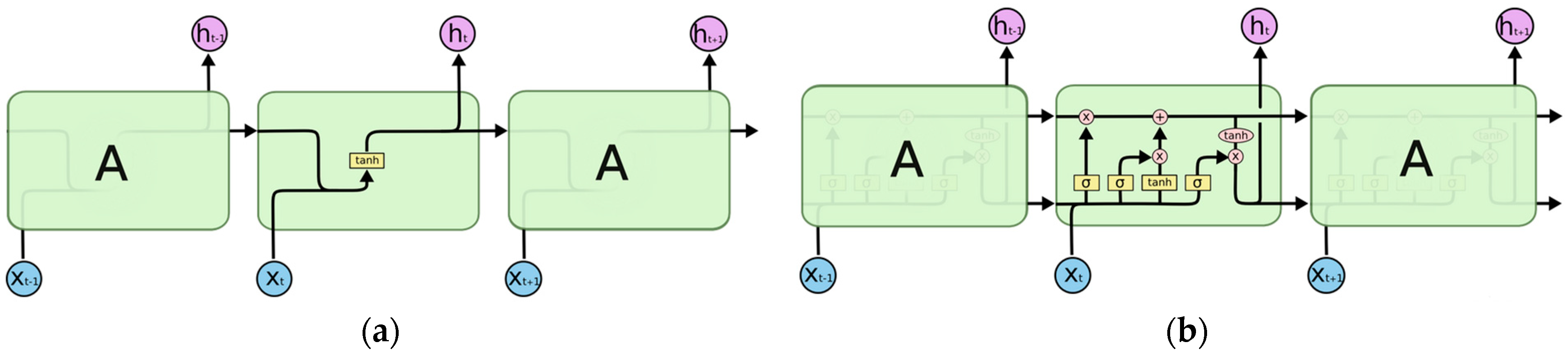
2.1. Long Short-Term Memory Principle

LSTMs, which were introduced by Hochreiter and Schmidhuber in 1997, were developed as a specialized type of a recurrent neural network (RNN) to address the challenges associated with vanishing or exploding gradients. These gradient issues limit the RNN’s ability to effectively capture long-term dependencies [34]. In contrast to the simple structure of an RNN with a single activation layer (Figure 1a), LSTMs have a more intricate architecture consisting of four layers (Figure 1b).

The LSTM architecture incorporates three controlling gates that protect and regulate the cell state:

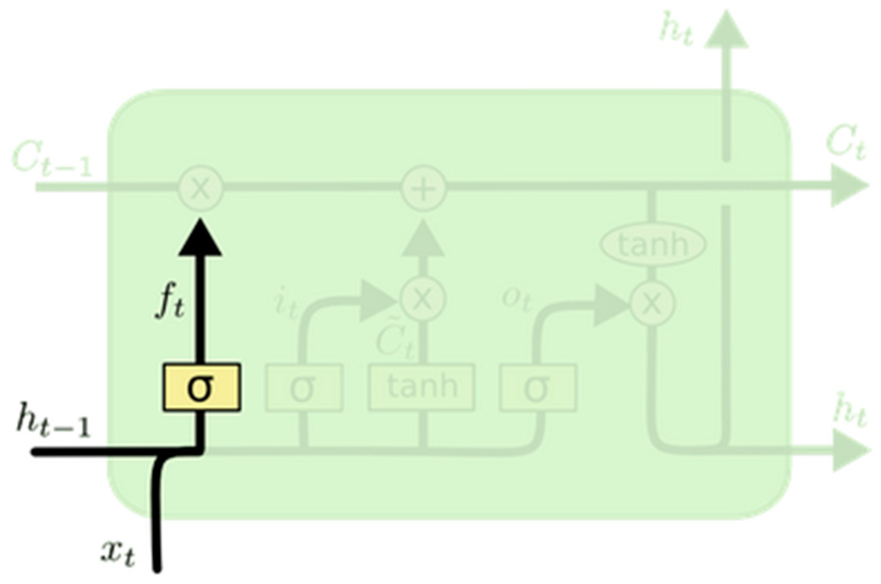
• Forget gate layer is a sigmoid layer that examines the input, $x_t$, and the previous hidden state. It generates a value between 0 and 1 to determine whether to retain or discard the information as illustrated by Equation (1) and Figure 2.

  $$f_t=\sigma \left(W_f\times \left[h_{t-1},x_t\right]+b_f\right),$$

  (1)

• The input gate layer consists of a sigmoid layer that decides which values should be updated based on Equation (2) and Figure 3. Additionally, it includes a hyperbolic tangent layer that generates a vector of new candidate values for the cell state using Equation (3) [34].

$$i_t=\sigma \left(W_i\times \left[h_{t-1},x_t\right]+b_i\right),$$

(2)

$${\tilde{C}}_t=tanh\left(W_c\times \left[h_{t-1},x_t\right]+b_c\right),$$

(3)

In this step, the previous cell state, $C$ at $t-1$, is updated to a new cell state, $C$ at $t$, by multiplying the old cell state by the output of the forget gate layer to determine what to retain. Then, the input gate layer outputs are multiplied to obtain the updated cell state, which is scaled based on the decision to update each value. Finally, the new cell state is added to the previous cell state using the pointwise addition operator, as illustrated in Equation (4) and Figure 3 [34].

$$C_t=f_t\times C_{t-1}+i_t\times {\tilde{C}}_t,$$

(4)

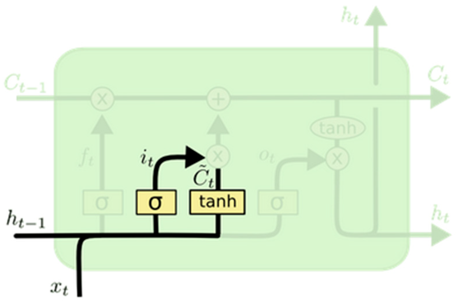
• The output gate layer is a sigmoid layer deciding which part of the cell state will be generated as output according to Equations (5) and (6) and as depicted in Figure 4.

$$o_t=\sigma \left(W_o\times \left[h_{t-1},x_t\right]+b_o\right),$$

(5)

$$h_t=o_t\times \mathrm{t}\mathrm{a}\mathrm{n}\mathrm{h}\left(C_t\right),$$

(6)

In the above equations, the parameters represent the following:

• $x_t$: the current time cycle input.
• $h_{t-1}$: the previous time cycle hidden state.
• W: the hidden state weight matrix.
• b: the input weight matrix.
• ${\tilde{C}}_t$: the cell input activation vector.
• $C_t$: the cell state vector.
• $\sigma$: the logistic sigmoid function expressed as in Equation (7) [22]:

  $$f\left(x\right)={\displaystyle \frac{1}{1+e^{-x}}}$$

  (7)

tanh: the hyperbolic tangent function presented in Equation (8) [22]:

$$h\left(x\right)={\displaystyle \frac{2}{1+e^{-x}}}-1$$

(8)

These properties make LSTM networks particularly suitable for predicting both hydraulic and water quality parameters, which often exhibit complex temporal dependencies. By leveraging LSTM’s ability to accurately forecast these parameters, water management systems can enhance their operational efficiency and ensure compliance with safety standards. This application underscores the significant potential of LSTM models in advancing water supply management.

2.2. Long Short-Term Memory Network

2.2.1. Study Area

The target study area is Incheon metropolitan city, Korea, where a red water accident occurred in 2019. For the investigation, real-time data were collected on flow discharge, water qualities (residual chlorine, conductivity, temperature, turbidity, and pH), and hydraulic pressure parameters from a district metered area (No. 845). The data used were the 2022 data provided by the Incheon Waterworks Business Headquarter, and the collection period was from 1 August to 30 September 2022, with a total of 1416 pieces of data collected on an hourly basis.

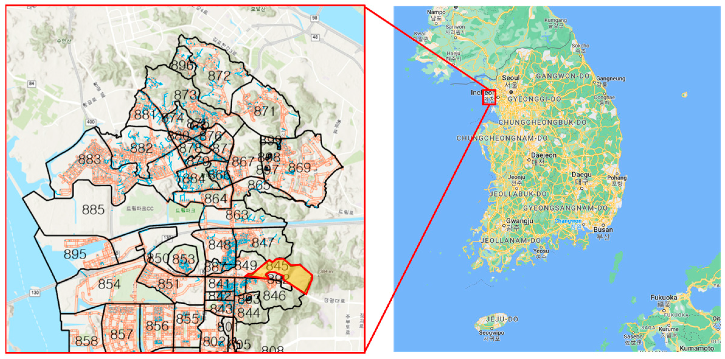
The water intake for district metered area (DMA) No. 845 is managed by Incheon Metropolitan city. This facility receives treated water from the Gongchon water treatment plant, which has a design capacity of 413,000 m³ per day and currently provides 309.8 m³ per day (Incheon Waterworks Business Headquarters, 2019). Figure 5, which illustrates the Target District Metered Area.

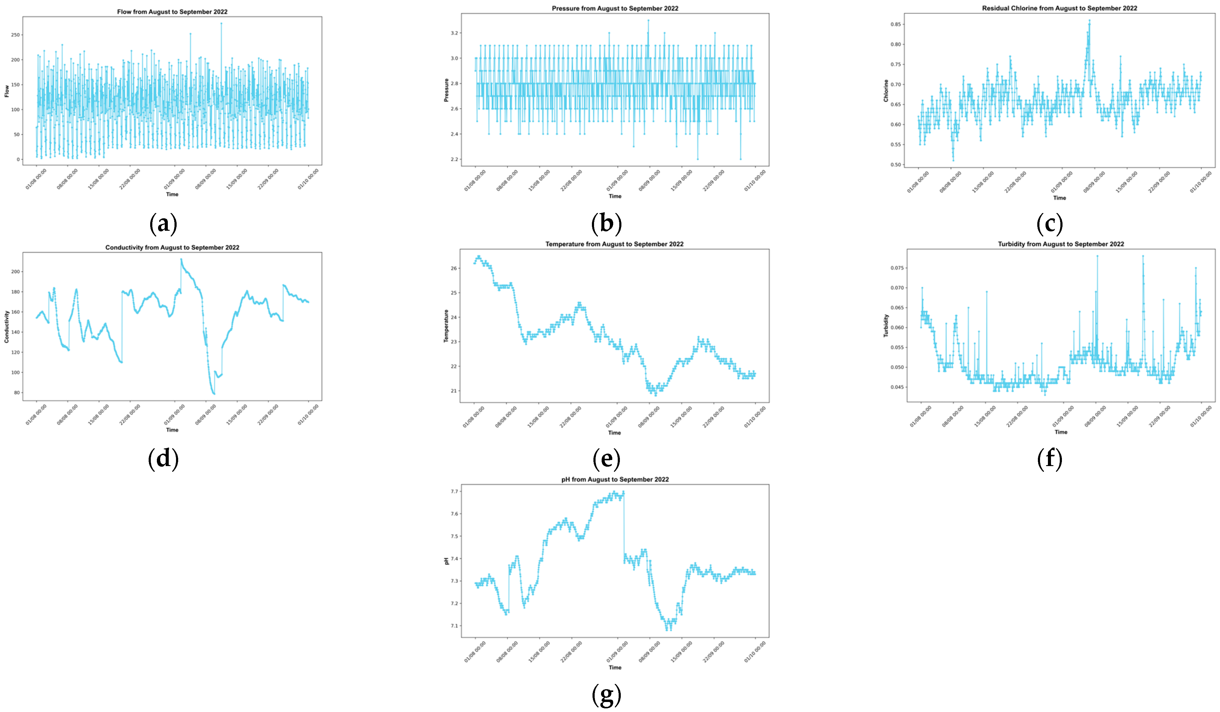
2.2.2. Input Data

To ensure the accuracy of our predictions and eliminate any potentially misleading values, the data for these months underwent preprocessing to address outliers and missing values. Outliers, defined as measurements that were not recorded or were erroneous due to communication issues, were corrected by interpolating from adjacent data points. The preprocessed data include measurements of flow discharge, residual chlorine, conductivity, temperature, turbidity, pH, and hydraulic pressure. These parameters are visually represented in Figure 6, which illustrates the trends and fluctuations in each parameter over the selected timeframe.

As shown in Figure 6, both flow discharge and hydraulic pressure show large daily changes and show a consistent pattern. In the case of residual chlorine, there is a daily pattern change, but trends appear depending on operation and temperature changes. In particular, the temperature is higher in August compared with September, so residual chlorine appears relatively low. In the case of conductivity, an irregular pattern appeared, and in the case of temperature, a clear decrease was seen over time. Turbidity and pH are greatly influenced by water purification plant water quality and pipe operation, and it is difficult to confirm seasonal changes.

In detail, for the discharge, the mean value was 104 m³/h, with a maximum of 273 m³/hr and a minimum of 2 m³/h. Significant variations were observed not only over the entire two-month period but also between day and night, indicating substantial fluctuations. In contrast, for pressure, the mean value was 2.8 Pa, with a maximum of 3.2 Pa and a minimum of 2.2 Pa, showing relatively smaller variations.

Among the water quality factors, conductivity exhibited a large standard deviation compared with the mean value. pH, on the other hand, had the smallest difference between the minimum and maximum values, with overall variations falling within a 10% range around the mean. Water quality factors showed more significant variations concerning the observation periods rather than on a daily basis. Particularly, turbidity demonstrated a noticeable trend, with daily fluctuations being relatively larger compared with other water quality factors.

Basic statistical results such as mean, minimum, maximum, and standard deviation values for each factor are shown in

Table 1. Basic statistical analysis.

Classification	Mean.	Min.	Max.	SD
Discharge (m3/h)	104.03	2.00	273.00	49.64
Pressure (Pa)	2.80	2.20	3.20	0.167
Residual chlorine (mg/L)	0.659	0.510	0.860	0.043
Conductivity (µS/cm)	157.59	78.60	212.40	24.76
Temperature (°C)	23.15	20.80	26.50	1.363
pH	7.380	7.080	7.700	0.153
Turbidity (NTU)	0.051	0.043	0.078	0.005

.

2.2.3. The Algorithm’s Parameters

In our study, the dataset was divided into two key subsets: a training set and a testing set. The last 24 data points were reserved for testing, ensuring the evaluation of the model’s performance on unseen data. This separation was crucial for assessing the model’s ability to generalize effectively beyond the data it had been trained on. The data were then normalized using the Min-Max scaling. This normalization procedure brought all the features within our dataset to a standardized scale to prevent any single feature from disproportionately influencing the model’s learning process due to differences in their scales, allowing the model to learn from all features more effectively [35].

The LSTM model was constructed using the Keras package 2.10.0 with TensorFlow 2.10.1 as back-end [36,37]. The network configuration was chosen through thorough experimentation. To facilitate the training of the LSTM model, a sequence-based approach was employed. Specifically, we employed the sliding window method to generate input–output pairs for the model, utilizing a window size of 24-time steps. This size was strategically chosen to encompass a full 24 h period, ensuring that the model captures all relevant daily patterns and fluctuations in the water-related parameters. This comprehensive view allows the model to make predictions with an informed understanding of the temporal dynamics presented by the preceding time steps, thus enhancing the accuracy and reliability of its forecasts.

The network consisted of one LSTM layer with 50 units and a hyperbolic tangent activation function. The output layer consisted of a single neuron with a linear activation function. The compilation of the model was executed with mean squared error (MSE) as the loss function and utilized the Adam optimizer to govern the model’s parameter adjustments during training. This optimizer was favored for its efficiency and robustness in the optimization process [38]. Additionally, to prevent overfitting, an early stopping callback was incorporated during training, which leveraged both the training and testing data.

The model underwent multiple iterations to yield the best possible results. The parameters that yielded the better results are summarized in

Table 2. LSTM model parameters.

LSTM	Dense	Batch Size	Epochs	Window Size
50	1	1000	500	24

.

In the evaluation of the LSTM prediction model, various performance metrics were employed to thoroughly assess its ability to reproduce observed data. These metrics include root mean squared error (RMSE), Nash–Sutcliffe efficiency (NSE), mean absolute error (MAE), percent bias (PBIAS), and coefficient of determination (R-squared), each serving a unique purpose in gauging different aspects of the model’s performance. The average magnitude of variations between expected and observed values can be understood by utilizing the RMSE. It provides a clear picture of the model’s capacity to replicate the observed data with the least amount of error by acting as a quantitative indicator of the overall accuracy of the model predictions [39].

NSE plays a pivotal role in evaluating the model’s prediction ability in relation to the observed data mean. A strong model fit is shown by a score near 1, which implies that the model successfully reflects the variability in the observed data. On the other hand, a score close to 0 indicates that the predictive power of the model is the same as if the observed data were used as a mean [40].The average absolute differences between predicted and observed values are measured by the MAE. This metric makes it possible to quickly evaluate how well the model reproduces the observed data by giving a clear indicator of its correctness [39]. The MAPE complements these metrics by providing insight into prediction accuracy expressed as a percentage. It measures the average magnitude of errors in predictions relative to actual values, allowing for an intuitive understanding of how well predictions align with observed data. A lower MAPE indicates better predictive performance, as it reflects smaller average percentage errors across all predictions.

The model’s systematic divergence from the observed values, or bias, is assessed using PBIAS. Model predictions that are in good agreement with the observed data are indicated by a PBIAS that is near to zero [41]. An all-encompassing picture of the model’s explanatory capacity is provided by R-squared, which indicates the percentage of variance in the observed data that the model can explain. A high level of explained variance is indicated by a number near to 1, which shows that the model can explain the underlying patterns in the observed data [42].

Together, these performance indicators offer a thorough evaluation of the LSTM prediction model, allowing for a detailed knowledge of both its strengths and places for development in terms of reproducing observed data.

$$RMSE=\sqrt{{\displaystyle \frac{1}{n}}{\sum }_{i=1}^n{\left(y_i-{\widehat{y}}_i\right)}^2},$$

(9)

$$\mathrm{N}SE=1-{\displaystyle \frac{{\sum }_{i=1}^n{\left(y_i-{\widehat{y}}_i\right)}^2}{{\sum }_{i=1}^n{\left(y_i-\overline{y}\right)}^2}},$$

(10)

$$\mathrm{MAE}={\displaystyle \frac{1}{n}}{\sum }_{i=1}^n\left|y_i-{\widehat{y}}_i\right|,$$

(11)

$$\mathrm{PBIAS}={\displaystyle \frac{{\sum }_{i=1}^n\left(y_i-{\widehat{y}}_i\right)}{{\sum }_{i=1}^n{y}_i}}\times 100,$$

(12)

$$\mathrm{MAPE}={\displaystyle \frac{1}{n}}{\sum }_{i=1}^n\left|{\displaystyle \frac{y_i-{\widehat{y}}_i}{y_i}}\right|\times 100,$$

(13)

$$R^2=1-{\displaystyle \frac{{\sum }_{i=1}^n{\left(y_i-{\widehat{y}}_i\right)}^2}{{\sum }_{i=1}^n{\left(y_i-\overline{y}\right)}^2}},$$

(14)

where:

• n: number of data points
• $y_i$: observed value of data point
• ${\widehat{y}}_i$: predicted value of data point
• ${\overline{y}}_i$: mean of observed values

3. Results

Predictions for a single day were made using LSTM based on two months’ worth of observed data during the summer season. Figure 7, Figure 8, Figure 9, Figure 10, Figure 11, Figure 12 and Figure 13 present the comparison of prediction accuracy for discharge, pressure, residual chlorine, conductivity, temperature, pH, and turbidity. For all the factors, a comparative analysis between the observed and predicted values was conducted using (a) line plots, (b) scatter plots, and (c) box plots. Performance metrics were summarized in

Table 3. Performance metrics.

Parameter	RMSE	R2	MAE	MAPE	NSE	PBIAS
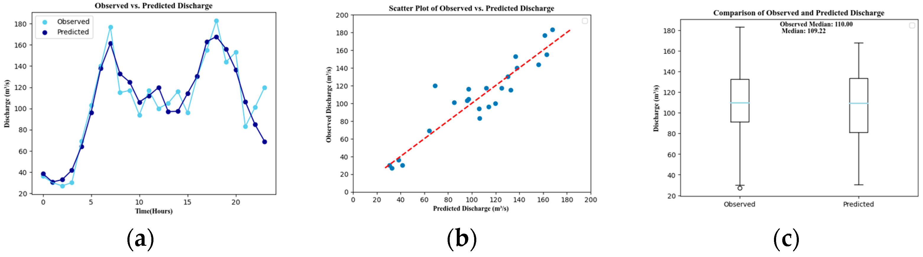
Discharge	16.205	0.857	12.499	13.103	0.857	−0.775
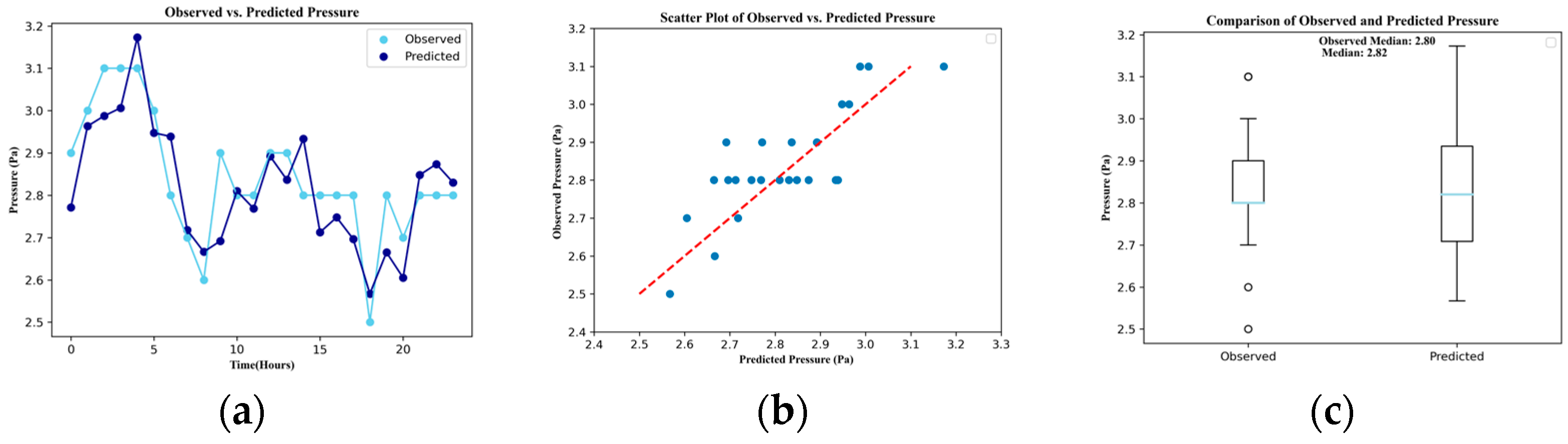
Pressure	0.091	0.600	0.077	2.734	0.600	−0.808
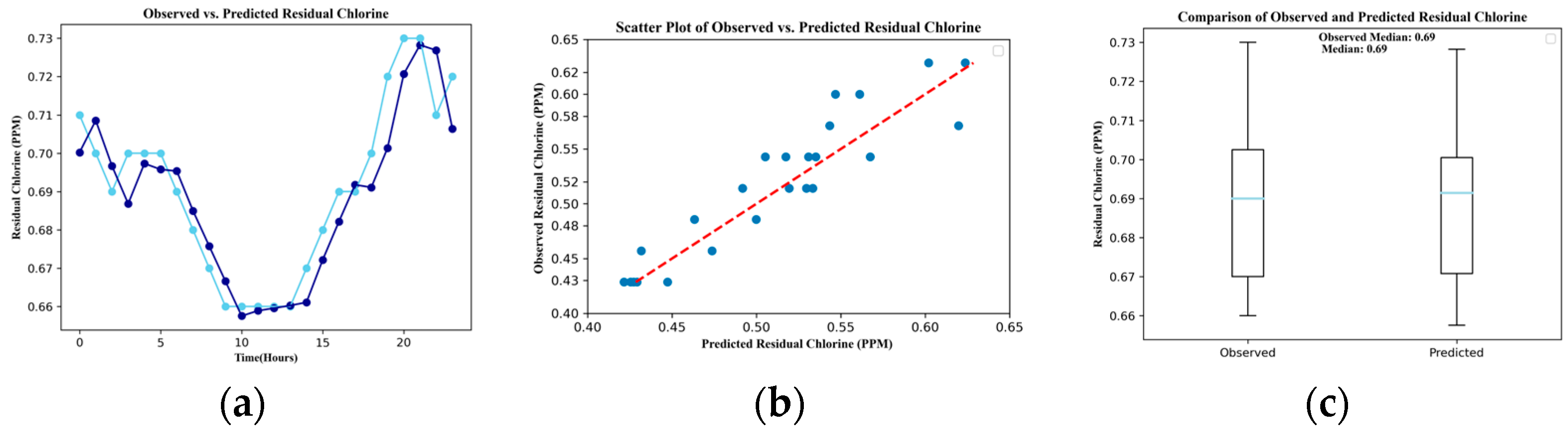
Residual chlorine	0.024	0.850	0.020	3.728	0.850	−1.243
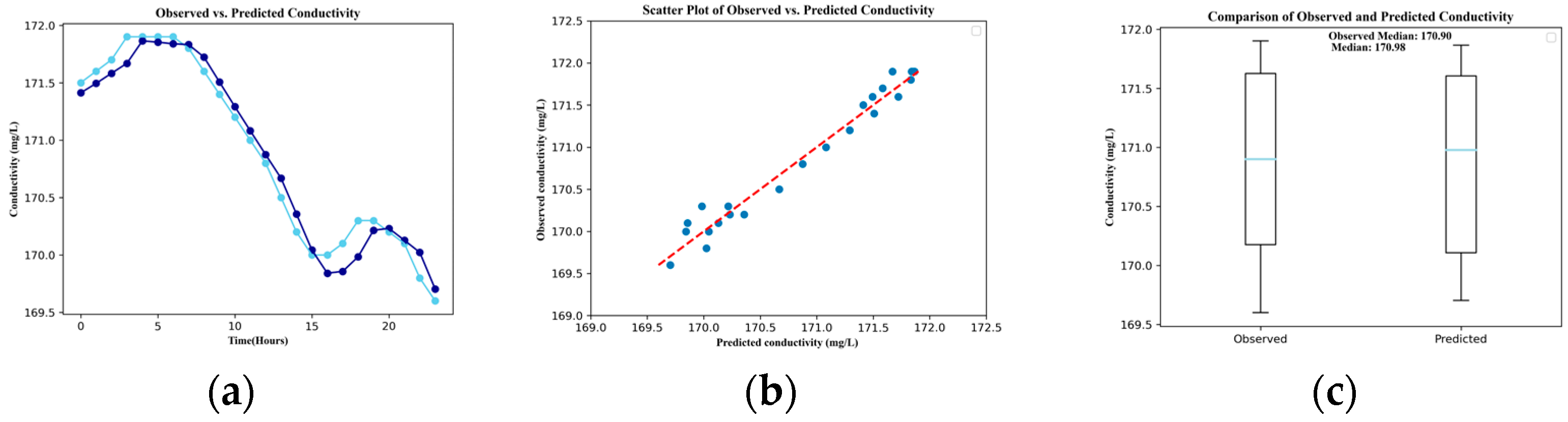
Conductivity	0.137	0.970	0.114	0.067	0.970	−0.005
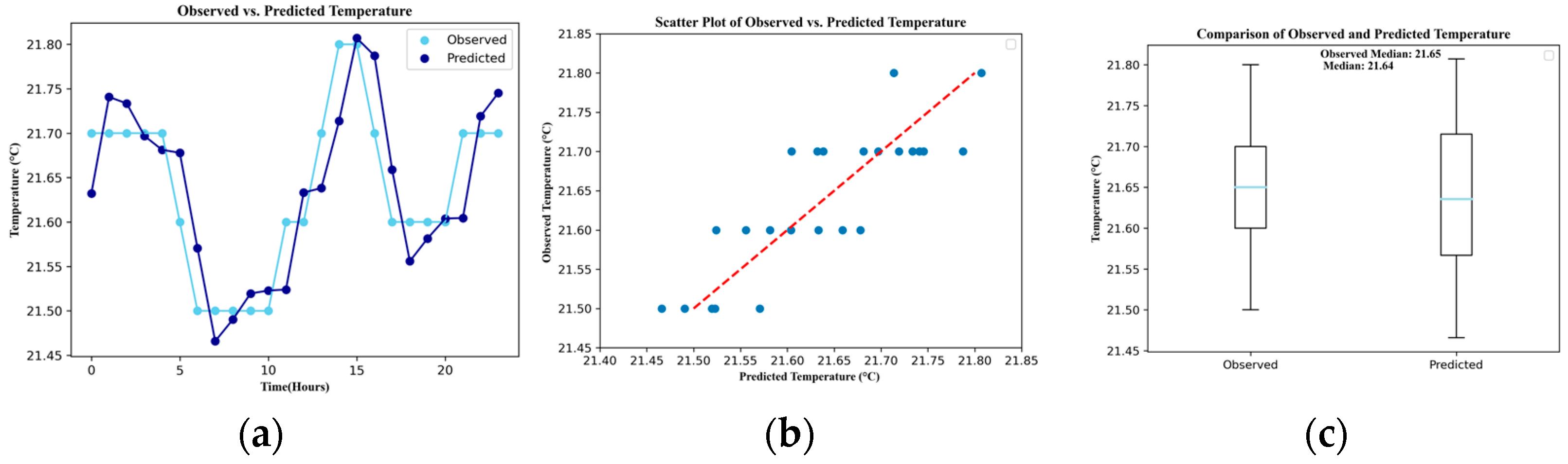
Temperature	0.052	0.673	0.043	0.199	0.673	0.000
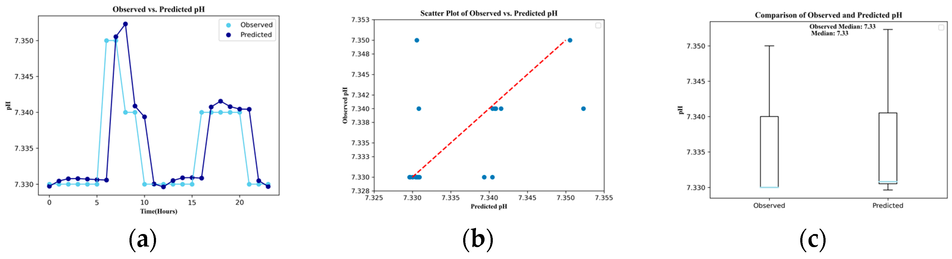
pH	0.005	0.178	0.003	0.041	0.178	0.008
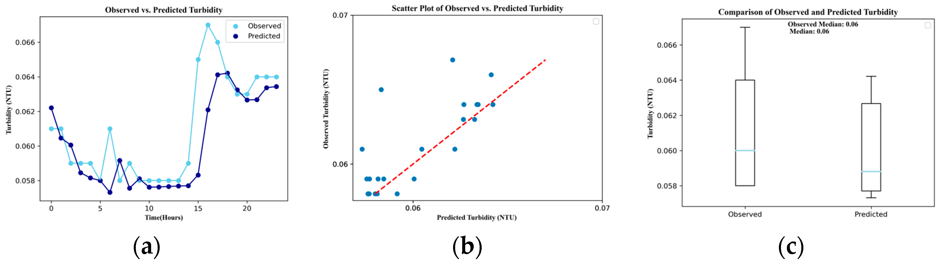
Turbidity	0.002	0.520	0.001	2.000	0.520	−1.512

. The observed versus predicted value plots provide a visual representation of the model’s performance in predicting various quality parameters, pressure, and discharge. The closer the data points lie to the diagonal line, the better the predictions align with the actual values in Figure 7b, Figure 8b, Figure 9b, Figure 10b, Figure 11b, Figure 12b and Figure 13b.

Discharge predictions stand out with exceptional accuracy, as evidenced by the close clustering of data points around the diagonal. This precision is further corroborated by low root mean square error (RMSE) and high R-squared (R²) values, indicating a robust linear relationship between predicted and observed discharge values. The MAPE of 13.103% suggests that, on average, predictions deviate from actual values by about 13%. Similarly, residual chlorine predictions showcase a strong alignment between the model’s predictions and actual values, reflected in low RMSE and high R² values, indicating a strong fit, while a MAPE of 3.728% reflects an excellent prediction accuracy with only a small average percentage error. The model also demonstrates exceptional accuracy in predicting conductivity. Data points closely align along the diagonal line, with remarkably low RMSE and high R² values underscoring its proficiency in capturing variations in ion concentrations within water. The MAPE for conductivity is notably low at 0.067%, indicating very precise predictions.

Pressure and temperature predictions, while not as precise as discharge, exhibit reasonable performance. The data points show a recognizable trend, albeit with some scattering, suggesting variability in predictions. The moderate R² value implies a moderate correlation between predicted and observed pressure. The MAPE for pressure is 2.734% and 0.199% for temperature. In contrast, turbidity and pH predictions present noticeable challenges. The scattered data points around the diagonal line and the low R² values collectively highlight the difficulty in accurately predicting these parameters. The MAPE for turbidity is 2.000%, while pH shows a MAPE of 0.041%.

The results for pH and discharge raise interesting points about interpreting statistical metrics in model evaluation. For pH, an R² value of 0.178 indicates a weak linear relationship between predicted and observed values, suggesting that the model does not capture important variability in pH measurements well. Although MAPE is low at 0.041%, indicating that individual predictions may be relatively close to observed values in percentage terms, this does not imply reliability or consistent trends across all observations.

In contrast, discharge has an R² value of 0.857, indicating a strong linear relationship where the model effectively captures trends in discharge data. However, a MAPE of 13.103% suggests that there are still instances where predictions significantly deviate from actual values on average.

To complement the visual assessment, a thorough statistical comparison of the observed and predicted data was conducted. A summary of these measures, including mean, median, and standard deviation, is presented in

Table 4. Statistical measures of the observed and predicted data.

Metric		Discharge	Pressure	Residual Chlorine	Conductivity	Temperature	pH	Turbidity
Mean	Obs.1	105.88	2.84	0.69	170.89	21.64	7.33	0.06
	Pred.2	105.05	2.82	0.69	170.88	21.64	7.34	0.06
Median	Obs.	110.00	2.80	0.69	170.90	21.65	7.33	0.06
	Pred.	109.22	2.82	0.69	170.98	21.64	7.33	0.06
Standard deviation	Obs.	42.95	0.86	0.02	0.79	0.02	0.09	0.08
	Pred.	40.90	0.14	0.02	0.77	0.02	0.09	0.07

Notes: ¹ Obs.: observed, ² Pred.: predicted.

.

The mean values, whether observed or predicted, exhibit a notable proximity. This close alignment indicates that the model capably captures the central tendencies of the data. It essentially means that the model is proficient in generating predictions that faithfully reflect the prevailing trends within the dataset. Similarly, the median values uncover a striking symmetry between the observed and predicted datasets. This symmetry underscores the absence of significant bias in the model’s predictions. Notably, the standard deviation, a measure of data variability, reveals an intriguing pattern. The standard deviation of predicted data consistently tends to be lower than that of the observed data. This divergence signifies that our model provides predictions with reduced variability, indicating a higher degree of prediction consistency.

In summation, the findings gleaned from this table underscore the model’s prowess in accurately capturing data trends, maintaining impartiality in its predictions, and delivering predictions with commendable consistency.

These findings align with those of previous studies, such as Kuhnert et al. [17], who demonstrated the superior accuracy of LSTM networks in predicting water demand for optimal pump control, and Liu et al. [18], who showed the effectiveness of LSTM models in analyzing and predicting water quality in an IoT environment. Additionally, Mu et al. [33] highlighted the robustness of LSTM models in accurately predicting both hourly and daily urban water demand.

Our study builds on this foundation by specifically focusing on the prediction accuracy of both hydraulic and water quality parameters using LSTM models. The consistency of our results with past research further validates the reliability of LSTM in this domain. The key contribution of our research lies in comparing the prediction accuracy of different water supply parameters, providing valuable insights for improving water resource management practices. This comparative analysis not only reinforces the applicability of LSTM models in complex data environments but also offers a detailed evaluation of their performance across various water-related factors, which is critical for informed decision-making in water management.

Furthermore, the results underline the necessity of optimizing LSTM parameters specific to each water quality and hydraulic factor. By refining these parameters, future research can achieve more accurate and timely predictions, thus significantly enhancing the model’s utility for real-time water management systems. This commitment to optimizing LSTM models will not only improve prediction accuracy but also enhance the operational efficiency of water resource management, as demonstrated by our comparative analysis of various water supply parameters.

4. Conclusions

In this study, we analyzed the accuracy of data prediction for future periods using the LSTM technique based on real-time monitoring data within the water supply network. LSTM has been widely applied across various fields, demonstrating high accuracy in predicting hydraulic and water quality data. In our study, it effectively predicted both hydraulic and water quality factors concerning daily pattern variations, and no outliers causing pattern changes were detected.

The results of our analysis showed that conductivity, discharge, and residual chlorine exhibited the highest accuracy, with R² values above 0.8. This high accuracy indicates significant advantages of applying the LSTM technique in water supply data prediction. Accurate predictions of these factors are crucial for monitoring water quality, ensuring compliance with standards, and safeguarding environmental sustainability. Specifically, changes in discharge can help predict leakage incidents, while residual chlorine and conductivity are key for predicting water quality incidents.

However, while overall predictions were successful, it was observed that when the magnitude of the data values is small, such as with turbidity and pH, the accuracy is compromised. This highlights the complexities involved in predicting these parameters and underscores the need for continued research to address these challenges. pH, influenced by intricate chemical reactions, remains a subject of interest and challenge within the field.

Additionally, our study relied on data collected during the summer months of August and September. For future research, we recommend exploring how water quality parameters fluctuate throughout the year to consider the influence of seasonal variations on data patterns. Expanding data collection to encompass multiple seasons will yield a more comprehensive understanding of temporal trends and facilitate the improvement of predictive models.

Furthermore, we acknowledge the need for parameter-specific optimization of LSTM learning parameters, as the use of a generalized model parameter set may have contributed to the observed delays in prediction results. Future studies will focus on identifying and applying optimal LSTM configurations for each specific water quality and hydraulic parameter, which is anticipated to enhance prediction accuracy and reduce potential delays.

In conclusion, our study provides valuable insights into water quality prediction, reflecting both successful outcomes and persistent challenges. The diverse performance of our predictive model across different water quality parameters offers valuable insights into the complexities of water quality prediction and highlights areas for improvement. These findings underscore the importance of data quality and model refinement. Future research endeavors will play a pivotal role in advancing our understanding of water quality and ensuring its sustained management and protection.

References

- Kavya, M.; Mathew, A.; Shekar, P.R.; Sarwesh, P. Short Term Water Demand Forecast Modelling Using Artificial Intelligence for Smart Water Management. Sustain. Cities Soc. 2023, 95, 104610. [Google Scholar] [CrossRef]
- Haghiabi, A.H.; Nasrolahi, A.H.; Parsaie, A. Water Quality Prediction Using Machine Learning Methods. Water Qual. Res. J. 2018, 53, 3–13. [Google Scholar] [CrossRef]
- Barzegar, R.; Asghari Moghaddam, A.; Adamowski, J.; Fijani, E. Comparison of Machine Learning Models for Predicting Fluoride Contamination in Groundwater. Stoch. Environ. Res. Risk Assess 2017, 31, 2705–2718. [Google Scholar] [CrossRef]
- Guo, G.; Liu, S.; Wu, Y.; Li, J.; Zhou, R.; Zhu, X. Short-Term Water Demand Forecast Based on Deep Learning Method. J. Water Resour. Plan. Manag. 2018, 144, 04018076. [Google Scholar] [CrossRef]
- Antunes, A.; Andrade-Campos, A.; Sardinha-Lourenço, A.; Oliveira, M.S. Short-Term Water Demand Forecasting Using Machine Learning Techniques. J. Hydroinform. 2018, 20, 1343–1366. [Google Scholar] [CrossRef]
- Bougadis, J.; Adamowski, K.; Diduch, R. Short-Term Municipal Water Demand Forecasting. Hydrol. Process. 2005, 19, 137–148. [Google Scholar] [CrossRef]
- Zhou, S.L.; McMahon, T.A.; Walton, A.; Lewis, J. Forecasting Daily Urban Water Demand: A Case Study of Melbourne. J. Hydrol. 2000, 236, 153–164. [Google Scholar] [CrossRef]
- Braun, M.; Bernard, T.; Piller, O.; Sedehizade, F. 24-Hours Demand Forecasting Based on SARIMA and Support Vector Machines. Procedia Eng. 2014, 89, 926–933. [Google Scholar] [CrossRef]
- Aissaoui, O.E.; El madani, Y.E.A.; Oughdir, L.; Allioui, Y.E. Combining Supervised and Unsupervised Machine Learning Algorithms to Predict the Learners’ Learning Styles. Procedia Comput. Sci. 2019, 148, 87–96. [Google Scholar] [CrossRef]
- Botvinick, M.; Ritter, S.; Wang, J.X.; Kurth-Nelson, Z.; Blundell, C.; Hassabis, D. Reinforcement Learning, Fast and Slow. Trends Cogn. Sci. 2019, 23, 408–422. [Google Scholar] [CrossRef]
- Taye, M.M. Understanding of Machine Learning with Deep Learning: Architectures, Workflow, Applications and Future Directions. Computers 2023, 12, 91. [Google Scholar] [CrossRef]
- Ahmed, S.F.; Alam, S.B.; Hassan, M.; Rozbu, M.R.; Ishtiak, T.; Rafa, N.; Mofijur, M.; Shawkat Ali, A.B.M.; Gandomi, A.H. Deep Learning Modelling Techniques: Current Progress, Applications, Advantages, and Challenges. Artif. Intell. Rev. 2023, 56, 13521–13617. [Google Scholar] [CrossRef]
- Najafabadi, M.M.; Villanustre, F.; Khoshgoftaar, T.M.; Seliya, N.; Wald, R.; Muharemagic, E. Deep Learning Applications and Challenges in Big Data Analytics. J. Big Data 2015, 2, 1. [Google Scholar] [CrossRef]
- Lecun, Y.; Bottou, L.; Bengio, Y.; Haffner, P. Gradient-Based Learning Applied to Document Recognition. Proc. IEEE 1998, 86, 2278–2324. [Google Scholar] [CrossRef]
- Mandic, D.; Chambers, J. Recurrent Neural Networks for Prediction: Learning Algorithms, Architectures and Stability; Wiley: Chichester, UK, 2001; ISBN 978-0-471-49517-8. [Google Scholar]
- Cho, K.; van Merrienboer, B.; Gulcehre, C.; Bahdanau, D.; Bougares, F.; Schwenk, H.; Bengio, Y. Learning Phrase Representations Using RNN Encoder-Decoder for Statistical Machine Translation. arXiv 2014, arXiv:1406.1078. [Google Scholar]
- Kuhnert, C.; Gonuguntla, N.; Krieg, H.; Nowak, D.; Thomas, J. Application of LSTM Networks for Water Demand Prediction in Optimal Pump Control. Water 2021, 13, 644. [Google Scholar] [CrossRef]
- Liu, P.; Wang, J.; Sangaiah, A.K.; Xie, Y.; Yin, X. Analysis and Prediction of Water Quality Using LSTM Deep Neural Networks in IoT Environment. Sustainability 2019, 11, 2058. [Google Scholar] [CrossRef]
- Nasser, A.; Rashad, M.; Hussein, S. A Two-Layer Water Demand Prediction System in Urban Areas Based on Micro-Services and LSTM Neural Networks. IEEE Access 2020, 8, 147647–147661. [Google Scholar] [CrossRef]
- Xu, Z.; Ying, Z.; Li, Y.; He, B.; Chen, Y. Pressure Prediction and Abnormal Working Conditions Detection of Water Supply Network Based on LSTM. Water Supply 2020, 20, 963–974. [Google Scholar] [CrossRef]
- Zanfei, A.; Brentan, B.; Menapace, A.; Righetti, M. A Short-Term Water Demand Forecasting Model Using Multivariate Long Short-Term Memory with Meteorological Data. J. Hydroinform. 2022, 24, 1053–1065. [Google Scholar] [CrossRef]
- Hochreiter, S.; Schmidhuber, J. Long Short-Term Memory. Neural Comput. 1997, 9, 1735–1780. [Google Scholar] [CrossRef] [PubMed]
- Purba, M.R.; Akter, M.; Ferdows, R.; Ahmed, F. A Hybrid Convolutional Long Short-Term Memory (CNN-LSTM) Based Natural Language Processing (NLP) Model for Sentiment Analysis of Customer Product Reviews in Bangla. J. Discret. Math. Sci. Cryptogr. 2022, 25, 2111–2120. [Google Scholar] [CrossRef]
- Lin, Y.; Lin, Z.; Liao, Y.; Li, Y.; Xu, J.; Yan, Y. Forecasting the Realized Volatility of Stock Price Index: A Hybrid Model Integrating CEEMDAN and LSTM. Expert Syst. Appl. 2022, 206, 117736. [Google Scholar] [CrossRef]
- Ghadekar, P.; Bongulwar, A.; Jadhav, A.; Ahire, R.; Dumbre, A.; Ali, S. Bi-LSTM Based Interdependent Prediction of Physiological Signals. In Proceedings of the 2023 International Conference on Emerging Smart Computing and Informatics (ESCI), Pune, India, 1–3 March 2023; pp. 1–6. [Google Scholar]
- Munagala, N.V.L.M.K.; Langoju, L.R.R.; Rani, A.D.; Reddy, D.V.R.K. A Smart IoT-Enabled Heart Disease Monitoring System Using Meta-Heuristic-Based Fuzzy-LSTM Model. Biocybern. Biomed. Eng. 2022, 42, 1183–1204. [Google Scholar] [CrossRef]
- Neog, H.; Dutta, P.E.; Medhi, N. Health Condition Prediction and Covid Risk Detection Using Healthcare 4.0 Techniques. Smart Health 2022, 26, 100322. [Google Scholar] [CrossRef]
- Oruh, J.; Viriri, S.; Adegun, A. Long Short-Term Memory Recurrent Neural Network for Automatic Speech Recognition. IEEE Access 2022, 10, 30069–30079. [Google Scholar] [CrossRef]
- Zhang, X.; Shi, J.; Yang, M.; Huang, X.; Usmani, A.S.; Chen, G.; Fu, J.; Huang, J.; Li, J. Real-Time Pipeline Leak Detection and Localization Using an Attention-Based LSTM Approach. Process Saf. Environ. Prot. 2023, 174, 460–472. [Google Scholar] [CrossRef]
- Kratzert, F.; Klotz, D.; Brenner, C.; Schulz, K.; Herrnegger, M. Rainfall–Runoff Modelling Using Long Short-Term Memory (LSTM) Networks. Hydrol. Earth Syst. Sci. 2018, 22, 6005–6022. [Google Scholar] [CrossRef]
- Zhang, J.; Zhu, Y.; Zhang, X.; Ye, M.; Yang, J. Developing a Long Short-Term Memory (LSTM) Based Model for Predicting Water Table Depth in Agricultural Areas. J. Hydrol. 2018, 561, 918–929. [Google Scholar] [CrossRef]
- Kammoun, M.; Kammoun, A.; Abid, M. LSTM-AE-WLDL: Unsupervised LSTM Auto-Encoders for Leak Detection and Location in Water Distribution Networks. Water Resour Manag. 2023, 37, 731–746. [Google Scholar] [CrossRef]
- Mu, L.; Zheng, F.; Tao, R.; Zhang, Q.; Kapelan, Z. Hourly and Daily Urban Water Demand Predictions Using a Long Short-Term Memory Based Model. J. Water Resour. Plan. Manag. 2020, 146, 05020017. [Google Scholar] [CrossRef]
- Olah, C. Understanding LSTM Networks. Available online: https://colah.github.io/posts/2015-08-Understanding-LSTMs/ (accessed on 26 September 2024).
- Patro, S.G.K.; Sahu, K.K. Normalization: A Preprocessing Stage. arXiv 2015, arXiv:1503.06462. [Google Scholar] [CrossRef]
- Team, K. Keras Documentation: LSTM Layer. Available online: https://keras.io/api/layers/recurrent_layers/lstm/#lstm-layer (accessed on 9 September 2023).
- Tf.Keras.Layers.LSTM|TensorFlow v2.13.0. Available online: https://www.tensorflow.org/api_docs/python/tf/keras/layers/LSTM (accessed on 9 September 2023).
- Chen, Z.C.; Zhang, Y.; Chen, W. Effective Adam-Optimized LSTM Neural Network for Electricity Price Forecasting | EndNote Click. Available online: https://click.endnote.com/viewer?doi=10.1109%2Ficsess.2018.8663710&token=WzM5OTg5MDksIjEwLjExMDkvaWNzZXNzLjIwMTguODY2MzcxMCJd.Gi79-GZTnwTfEjmlGD7s1Mah4nI (accessed on 23 October 2023).
- Chai, T.; Draxler, R. Root Mean Square Error (RMSE) or Mean Absolute Error (MAE)? Geosci. Model Dev. 2014, 7, 1525–1534. [Google Scholar] [CrossRef]
- Gupta, H.V.; Kling, H. On Typical Range, Sensitivity, and Normalization of Mean Squared Error and Nash-Sutcliffe Efficiency Type Metrics. Available online: https://agupubs.onlinelibrary.wiley.com/doi/10.1029/2011WR010962 (accessed on 22 November 2023).
- Madsen, T.; Franz, K.; Hogue, T. Evaluation of a Distributed Streamflow Forecast Model at Multiple Watershed Scales. Water 2020, 12, 1279. [Google Scholar] [CrossRef]
- Colin Cameron, A.; Windmeijer, F.A.G. An R-Squared Measure of Goodness of Fit for Some Common Nonlinear Regression Models. J. Econom. 1997, 77, 329–342. [Google Scholar] [CrossRef]