Article

Combining SWAT with Machine Learning to Identify Primary Controlling Factors and Their Impacts on Non-Point Source Pollution

1
School of Civil & Environmental Engineering and Geography Science, Ningbo University, Ningbo 315211, China
2
Ningbo City Reservoir Management Center, Ningbo 315020, China
3
Zhejiang Ningbo Ecological and Environmental Monitoring Center, Ningbo 315012, China
*
Authors to whom correspondence should be addressed.
Water 2024, 16(21), 3026; https://doi.org/10.3390/w16213026
Submission received: 30 September 2024 / Revised: 19 October 2024 / Accepted: 21 October 2024 / Published: 22 October 2024
(This article belongs to the Section Water Quality and Contamination)

Abstract

:
Non-point source (NPS) pollution has a complex formation mechanism, and identifying its primary controlling factors is crucial for effective pollution treatment. In this study, the Baixi Reservoir Watershed, characterized by low-intensity development, was selected as the study area. A new methodology combining the Soil and Water Assessment Tool (SWAT) with the Random Forest (RF) algorithm was proposed to comprehensively identify the primary controlling factors of NPS pollution and analyze the interaction between factors. The results of the validated SWAT model showed that the annual intensity of total nitrogen (TN) load range was 0.677–11.014 kg ha−1 yr−1, and the total phosphorus (TP) load per unit area range was 0.020–0.110 kg ha−1 yr−1. Loads of sediment, TP, and TN exhibited significant seasonal variations, particularly in the Baixi basin, where sediment yield had the highest absolute change rate, with a value of up to 232.26. Random Forest models for TN and TP displayed high accuracy (R2 > 0.99) and robust generalization ability. Fertilization, sediment yield, and terrain slope were identified through RF models as the primary factors affecting TN and TP. By graphing partial dependency plots (PDPs) based on the results of the RF models to analyze the interaction between factors, the findings suggest a strong synergistic effect of two combined factors: fertilization and sediment yield. When fertilizer application exceeds 15 kg ha−1 yr−1 and sediment yield exceeds 3 kg ha−1 yr−1, there is a sharp increase in nitrogen and phosphorus load. Through the identification and analysis of the primary controlling factors of NPS pollution, this study provides a solid scientific foundation for developing effective watershed management strategies.

1. Introduction

In recent years, with effective control of industrial and urban wastewater, non-point source (NPS) pollution has become a significant threat to water quality [1]. NPS pollution not only degrades water quality but also poses significant risks to human health and aquatic ecosystems. Sources of NPS pollution, such as agricultural runoff, urban stormwater, and atmospheric deposition, often contain excessive nutrients (nitrogen and phosphorus) and harmful chemicals (e.g., pesticides). These pollutants can lead to eutrophication, resulting in harmful algal blooms that deplete oxygen levels in water bodies, creating hypoxic or “dead zones” that are detrimental to aquatic life [2,3]. The loss of biodiversity and the potential mortality of aquatic species, particularly fish, can destabilize ecosystems. Furthermore, NPS pollution can contaminate drinking water sources, leading to serious public health risks. For instance, toxins produced by cyanobacteria (harmful algae) in eutrophic waters are linked to liver damage and neurological disorders and may even increase the risk of certain cancers [4,5]. In addition to health hazards, the degradation of water quality also has economic repercussions, particularly in regions where fisheries, irrigation, and tourism rely heavily on reservoirs. The economic losses associated with NPS pollution in these sectors can be substantial [6]. NPS pollution is widely recognized as a major environmental concern due to its diffuse nature, irregular discharge patterns, and complex transport mechanisms, making it difficult to monitor and control [7,8,9]. Reservoirs, as primary water sources for society, are particularly vulnerable to NPS pollution. Their closed hydrological systems and limited water exchange capacity result in weak self-purification, increasing their vulnerability to issues like drinking water contamination and eutrophication [10,11,12]. Currently, monitoring and treatment efforts are focused primarily on reservoirs. Therefore, it is crucial to explore the main factors influencing NPS pollution from a watershed perspective and address the root causes of the issue.
There are several simplified methods to identify the primary controlling factors of NPS pollution, such as linear regression analysis, multivariate analysis of variance, and correlation analysis [13,14,15,16]. However, these traditional analytical methods are limited in their ability to comprehensively capture and analyze the interactions between various factors and their compounded effects on NPS pollution [17]. Furthermore, the scarcity of field-measured data poses additional challenges for conducting a comprehensive analysis of the causes of NPS pollution [18]. All of these factors have restricted the comprehensive understanding and evaluation of the deeper impact mechanisms of NPS pollution.
In the exploration of multi-factor interactions, machine learning (ML) provides powerful methods for analyzing complex data. Certain ML models, such as Random Forest (RF), when combined with appropriate preprocessing techniques, are particularly effective in managing challenges like multicollinearity, outliers, and noise. The RF algorithm’s strength lies in its ability to aggregate predictions from multiple decision trees, each built from random subsets of the training data, making it widely used in both classification and regression tasks [19]. In environmental research, RF has been successfully applied to analyze factors influencing heavy metal pollution [20], soil erosion [21,22], and agricultural management practices [23]. Additionally, the Soil and Water Assessment Tool (SWAT) model, an advanced hydrological simulation tool, can effectively simulate the processes of runoff, sediment, and nutrient transport within a watershed, providing robust support for research on NPS pollution [24,25,26]. The SWAT model is applicable across various domains, including land use changes [27,28] and climate change impact assessments [29], covering watersheds in many regions globally.
The combination of the SWAT model with machine learning methods has been applied in NPS pollution management [30,31]. However, these studies have primarily focused on using the model to simulate core indicators, such as runoff and nitrogen and phosphorus loads, for ecological evaluation. They have not fully utilized or integrated the comprehensive data resources provided by the SWAT model, such as land use types, terrain slope, sediment yield, and water yield. Additionally, the complexity of key influencing factors has not been sufficiently considered when using SWAT model data [32]. Therefore, a multidimensional and in-depth analysis of NPS pollution-influencing factors, particularly the exploration of how complex environmental elements interact and jointly drive the NPS pollution process, remains an area that warrants further investigation.
In this study, a new methodology was used that employed key data simulated by a validated SWAT model, in combination with the Random Forest algorithm, to comprehensively reveal the spatiotemporal distribution characteristics of NPS pollution and analyze its primary controlling factors. This research provides a robust scientific foundation for developing effective water management strategies and highlights the unique value of integrating machine learning and statistical analysis in environmental science research.

2. Data and Methods

2.1. Study Area

Baixi Reservoir, located in the eastern coastal region of China, serves as an important drinking water source for Ningbo City, with a total storage capacity of 168 million cubic meters and a watershed area of 252 square kilometers (121°04′ E to 121°18′ E and 29°11′ N to 29°22′ N) (Figure 1a). The watershed contains two main rivers—Baixi River and Dasongxi River, along with their seven tributaries. The Baixi River, extending about 100 km in length, flows through a landscape where the mountains predominantly trend northwest-to-southeast, with terrain sloping from high in the west to low in the east. The Baixi Reservoir Watershed experiences a subtropical monsoon climate, characterized by an average annual temperature of 16.1 °C and an average annual precipitation of 1838.9 mm, with 46.8% of the annual precipitation occurring between June and August. This region could be characterized as a mountainous area with agricultural vegetation, secondary forest, and productive forest [33]. The land use in the watershed is distributed as follows: 88.27% forest, 7.16% cropland, 1.89% water area, 1.32% orchard, 0.73% grassland, 0.60% construction land, and 0.03% other land, as illustrated in Figure 1b.
There is a permanent resident population of about 8000 people in the Baixi Reservoir Watershed, with no industrial facilities, and most of the domestic sewage is treated by the treatment terminal. Overall, point source pollution of the Baixi Reservoir Watershed has been treated, classifying the study area as a low-intensity development watershed. However, the upstream catchment area of the reservoir presents challenges attributed to soil erosion and concentrated cropland areas, leading to nitrogen and phosphorus pollution loads from non-point sources, which brings significant risk to the reservoir’s aquatic environment and drinking water supply safety.

2.2. SWAT Model Data Sources and Processing

To establish the SWAT model, long-term data spanning from 2008 to 2024, including the Digital Elevation Model (DEM), land use, soil types, meteorological data, water quality, and other relevant factors within the Baixi Reservoir Watershed, were collected for this study. Land use data were sourced from the Ningbo Municipal Bureau of Land and Resources and further refined through calibration using remote sensing data specific to the watershed. Meteorological data, including daily precipitation, temperature, relative humidity, solar radiation, and wind speed, were provided by the Ningbo Meteorological Bureau. Water quality data were detected and collected at the monitoring station. The locations of the meteorological, monitoring, and hydrological stations are shown in Figure 1a. Fertilization practices within the Baixi Reservoir Watershed were documented based on agricultural annual reports from the towns of Huangtan and Chalu. The types and sources of all these data are summarized in Table 1.
In this study, the SWAT model was used to divide the Baixi Reservoir Watershed into 18 sub-watersheds. Based on the two tributaries flowing into the Baixi Reservoir, the watershed was further divided into three smaller watersheds: the Dasongxi Basin, the Baixi Basin and the Reservoir Basin, as shown in Figure 1c. The SWAT model refines each sub-watershed into several hydrologic response units (HRUs) based on land use types, soil types, and slope categories. Slopes were categorized into three levels: 0−15°, 15−25°, and >25° in the Baixi Reservoir Watershed. The threshold values for land use types, soil types, and slope levels were set at 2%, 10%, and 10%, respectively. Consequently, the whole watershed was subdivided into 230 HRUs. After simplification, four types of land use, namely cropland (RICE), forest land (FRST), orchard (ORCD), and water area (WATR), were retained.
The SWAT model employs numerous parameters to depict watershed characteristics, and the accuracy of the model is influenced by spatial variations in parameters and errors incurred during their acquisition [41]. For this purpose, the SWAT model was calibrated and validated using long-term measured data of monthly average flow discharge, NH3-N, TN, and TP from January 2011 to May 2024, which were provided by the Baixi Reservoir Management Station. In the simulation process, the model’s warm-up period was from January 2008 to December 2010, its calibration period was from January 2011 to December 2020, and its validation period was from January 2021 to May 2024. The SUFI2 [42] method in SWAT-CUP (SWAT Calibration and Uncertainty Procedures) was applied for optimizing and adjusting the main parameters affecting pollutant output, followed by sensitivity analysis and model calibration adjustments.

2.3. SWAT Model Calibration

In this study, 26 key parameters were selected, involving vegetation and management, soil, nutrient transport, hydrological process, groundwater, and channel and erosion. The comprehensive sensitivity rankings and fitted values are presented in Table 2. The specific description of the parameters is shown in Table S1.
To assess the accuracy and applicability of the SWAT model, the determination coefficient (R2) and Nash–Sutcliffe Efficiency coefficient (NSE) were employed. A model is considered accurate and applicable in the study area if R2 ≥ 0.6 and NSE ≥ 0.5 [43].

2.4. Calculation of TN and TP

In this study, statistical analyses of 230 HRUs in the Baixi Reservoir Watershed were conducted on a monthly time scale, examining the relationships between various environmental factors (meteorological, spatial data, etc.) and response factors (TN and TP). TN and TP were calculated according to the relevant output data of the SWAT model:
TN = ORGN + NSURQ + NLATQ + NO3GW
TP = ORGP + SOLP + SEDP + P_GW
where ORGN represents organic nitrogen output, NSURQ is surface-flow nitrate output, NLATQ is lateral-flow nitrate output, NO3GW is groundwater nitrate output, ORGP is organic phosphorus output, SOLP is surface-flow-soluble phosphorus output, SEDP is sediment phosphorus output, and P_GW is groundwater-soluble phosphorus output.

2.5. The Coefficient of Variation (CV) and Absolute Change Rate ( α )

To reveal the intra-annual distribution unevenness of sediment yield, water yield, TP load, and TN load within the watershed, this study used the CV and α to assess the degree of dispersion in the data from different perspectives.
The formula for calculating the Coefficient of Variation (CV) is as follows:
C v = δ R ¯ = 1 n × i = 1 n ( R i R ¯ ) 2 R ¯
R ¯ = 1 n × i = 1 n R i
where R ¯ represents the annual mean value; R i is the value for the i month within the year. The value of the CV indicates the degree of deviation of each indicator’s distribution relative to the mean. A smaller CV signifies a more even distribution of the data throughout the year.
The formula for absolute change rate ( α ) is as follows:
α = R m a x R m i n
where R m a x and R m i n represent the maximum and minimum values within the year, respectively. The absolute change rate reflects the multiple relationship between extreme values, indicating the degree of unevenness. The larger the absolute change rate, the more uneven the distribution of the data throughout the year.

2.6. Random Forest Modeling

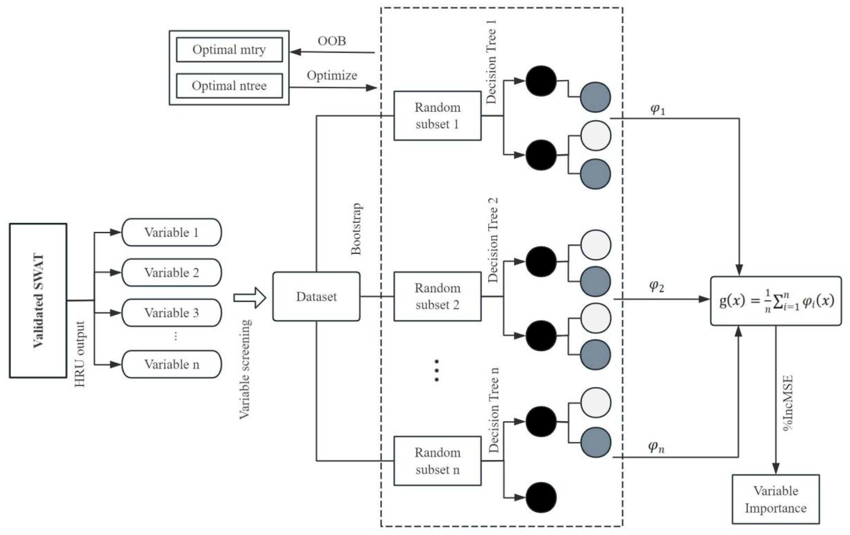
To identify the key factors influencing NPS pollution and uncover the complex relationships between these factors, we employed the Random Forest algorithm in R 4.3.2, an machine learning method introduced by Breiman in 2001 [19]. The RF modeling process includes feature selection, data preprocessing, model training, and hyperparameter optimization [44], as shown in Figure 2.
Initially, based on the HRU, SUB, and RCH output files from the SWAT model and drawing on related studies on NPS pollution [45,46,47], we pre-selected 18 parameters that significantly impact nitrogen and phosphorus. After conducting correlation analysis and multicollinearity tests, 11 key parameters were chosen for modeling. These parameters included four land use types, terrain slope, water yield, average temperature, fertilizer amount, solar radiation, initial soil moisture, and sediment yield. The dataset consisted of monthly average values from January 2011 to May 2024, calculated for 230 HRUs. This resulted in 12 monthly values for each HRU, totaling 2760 records. The monthly average values of the 11 parameters and TN/TP loads for different watersheds are shown in Table S2.
During the data preprocessing stage, missing values and obvious outliers were removed. Bootstrap sampling was then employed to create a new subset by sampling with replacement from the cleaned data set, while the unsampled portion was designated as the out-of-bag (OOB) data. A regression tree was constructed using each bootstrap sample, and this process was iterated multiple times to build several regression trees. The OOB data was utilized to determine the optimal number of trees.
The model’s key hyperparameters included ntree (the number of trees) and mtry (the number of variables considered at each split). The optimal value for mtry was determined using five-fold cross-validation, where performance metrics such as RMSE, R2, and MAE were considered. As shown in Table S3, mtry = 5 provided the best balance of performance. The generalization error of the RF model decreases as ntree increases, ensuring stability with a sufficiently large ntree. However, setting ntree too high can reduce efficiency. Based on Figure S1, ntree = 500 was chosen, while other parameters were kept at their default settings. With these determined parameters, the Random Forest models for TN and TP were constructed, and the final output was obtained by averaging the predictions from all the trees.
Finally, to evaluate the importance of each variable in the Random Forest model, we analyzed the change in mean squared error (MSE) when each variable was randomly permuted in the OOB data. This method involves shuffling the values of a single variable and measuring the resulting increase in MSE compared to the original model. A higher %IncMSE indicates that the variable is more important, as its absence significantly reduces the model’s predictive accuracy.

2.7. Partial Dependency Plot (PDP)

PDPs are a visualization tool used to interpret the feature importance and effects in machine learning models. PDPs help with understanding how the model responds to changes in a single feature or a set of features and can reveal the relationships between these features and the model predictions [48]. In this study, the vivid package [49] in R 4.3.2 software was used to generate PDPs for further analysis. Equation (6) presents the formula for a PDP.
f s x s = 1 n i = 1 n g x s , x c i
where f s x s represents the partial dependency of the model prediction on the feature subset x s , n is the number of observations, x c i denotes the remaining features not included in x s , and g ( ) is the predicted output of machine learning model.

3. Results and Discussion

3.1. SWAT Model Validation

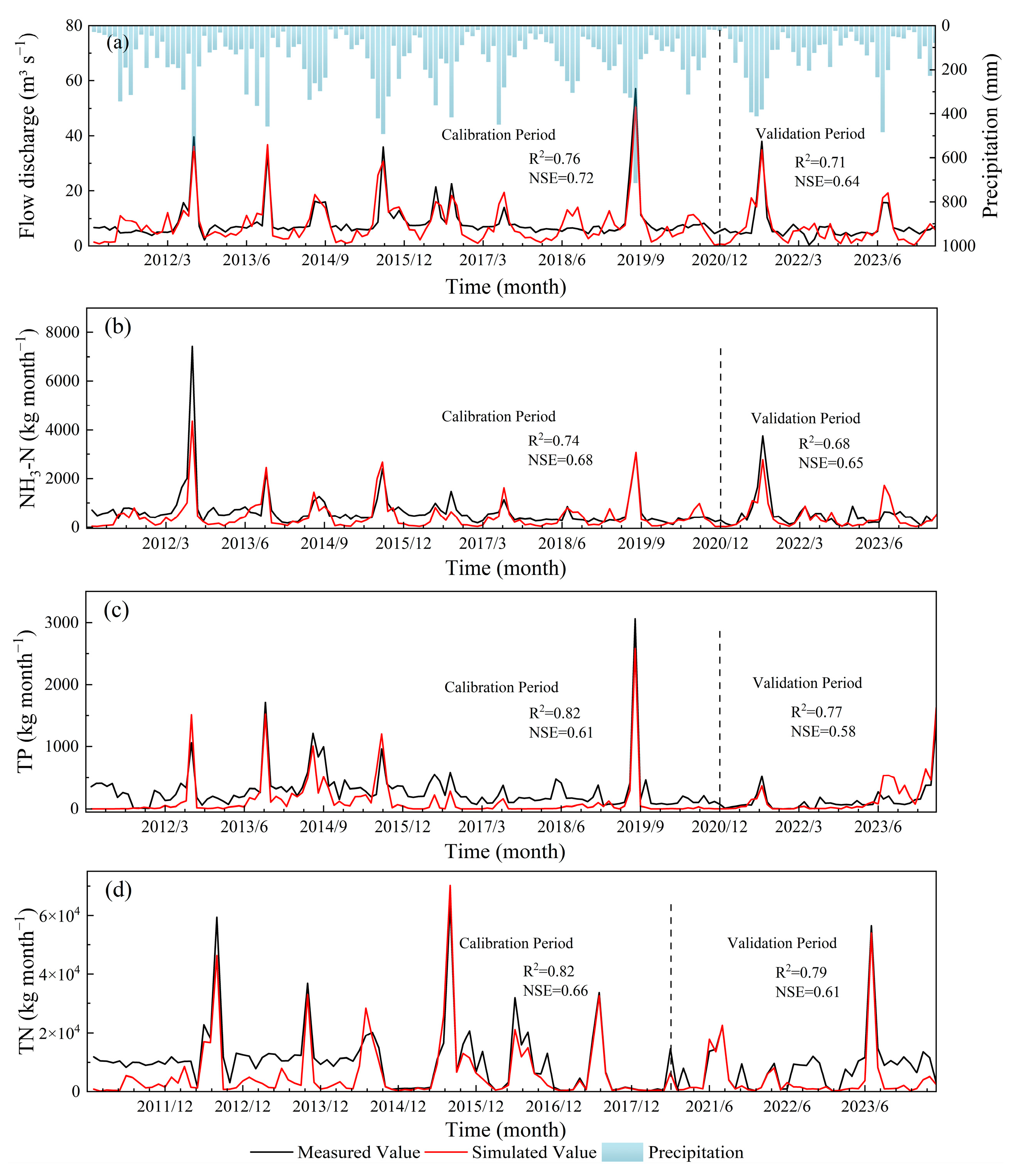
The model’s performance was evaluated during the calibration (January 2011–December 2020) and validation (January 2021–May 2024) periods, with the results summarized in Figure 3. Among them, the calibration period for TN is from January 2011 to June 2018, and the validation period is from January 2021 to May 2024.
The results show that the model exhibited satisfactory performance in simulating flow discharge, NH3-N, TP, and TN, with R2 and NSE values meeting or exceeding the defined thresholds. The R2 values during the calibration period for flow discharge, NH3-N, TP, and TN, ranged from 0.74 to 0.82, all of which exceeded the standard value of 0.6, as did the R2 values in the validation period, which ranged from 0.68 to 0.79. The NSE values in the calibration period for flow discharge, NH3-N, TP, and TN, were in the range of 0.61–0.72, which exceeded the standard value of 0.5, as did those in the validation period, which were in the range of 0.58–0.65. Consequently, from an overall perspective of flow discharge, NH3-N, TP, and TN simulations, the calibrated SWAT model was proved suitable for the simulation of NPS pollution in the Baixi Reservoir Watershed.

3.2. Spatiotemporal Distribution of NPS in the Watershed

3.2.1. Temporal Distribution of NPS

Analyzing the monthly variation is crucial for identifying pollution sources, protecting water quality, and assessing ecological impacts. Monthly simulated values for sediment yield (SYLD), water yield (WYLD), TP load, and TN load were extracted from the output results of the validated SWAT model. The seasonal variations, the coefficient of variation, and the absolute change rate are depicted in Figure 4.
The results demonstrated significant seasonal variations in sediment yield, water yield, TP load, and TN load. The trends in TP and TN loads closely mirrored those of sediment yield and water yield. An analysis of the monthly average data revealed that, in spring, especially in March, peak values of sediment, TP load, and TN load were primarily driven by meteorological conditions and spring plowing. After May, sediment yield declined significantly due to reduced soil erodibility and the recovery of vegetation [50]. Further analysis of surface runoff data supported these findings, with the average runoff in March recorded at 2.22 mm, while runoff in April and May was less than 0.7 mm, further validating the observed reduction in sediment yield. From June to August, the total outputs of sediment yield, water yield, TP load, and TN load in the Baixi Reservoir Watershed accounted for 70.19%, 50.16%, 70.08%, and 64.50% of the annual totals, respectively. Additionally, in August, peak monthly loads were observed, with sediment reaching 6845.09 tons month−1, water yield at 49,375,732.84 m3 month−1, TP load at 697.08 kg month−1, and TN load at 31,795.18 kg month−1.
Analyzing the monthly variation coefficients across different basins revealed that the CV of water yield is the lowest among these parameters, indicating that water yield exhibits the smallest fluctuation throughout the year. In contrast, the average values of CV are 1.28 for sediment yield, 1.40 for TP load, and 1.03 for TN load, suggesting greater variability compared to that of water yield. Despite similar CV values across different watersheds, the absolute change rates vary, particularly in the Baixi basin, where sediment yield has the highest absolute change rate of 232.26. This indicates a higher susceptibility to soil erosion in the Baixi basin under extreme conditions.

3.2.2. Spatial Distribution of NPS

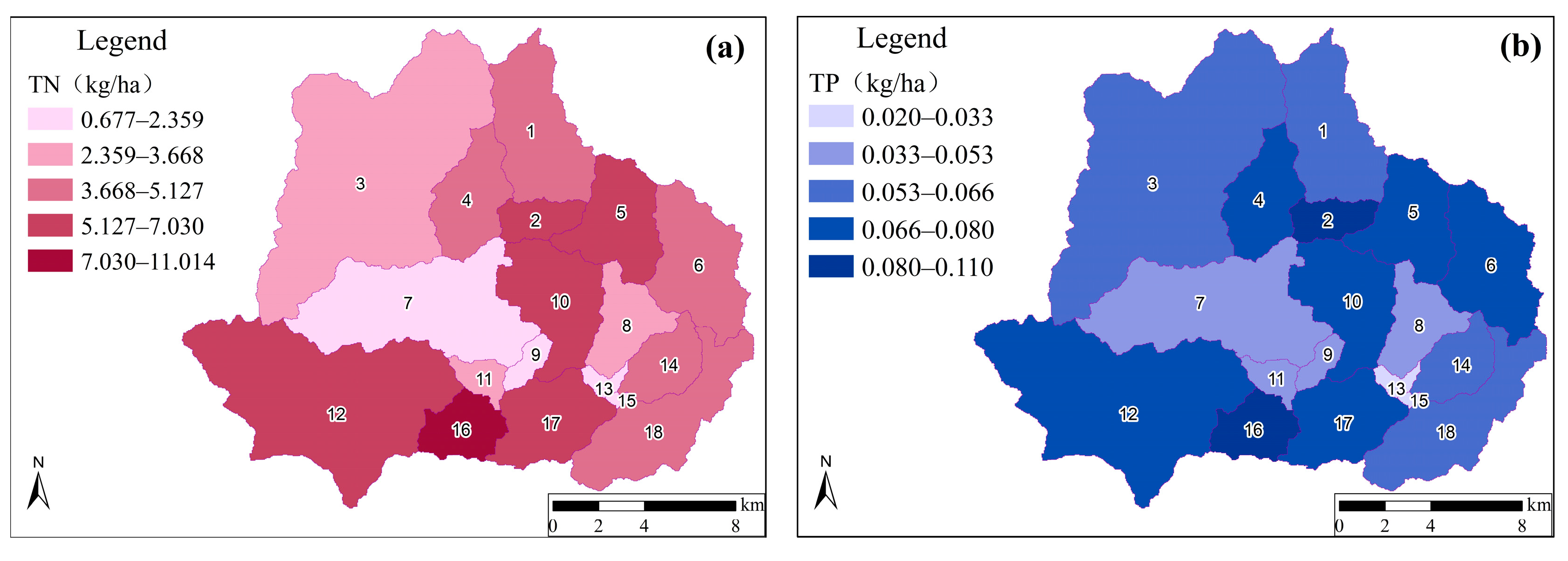
By extracting watershed output data from the validated SWAT model of the Baixi Reservoir Watershed and combining it with GIS spatial analysis functionality, the spatial distribution of nitrogen and phosphorus pollution load outputs across each sub-watershed was obtained and mapped, as shown in Figure 5.
According to the spatial statistical results of annual average pollution load, NPS pollutant load, e.g., TN and NP, exhibits strong spatial characteristics in the study area. The annual load intensities of TN in each sub-watershed ranged from 0.677 to 11.014 kg ha−1 yr−1, and those of TP ranged from 0.02 to 0.11 kg ha−1 yr−1, with mean values of 4.51 kg ha−1 yr−1 and 0.06 kg ha−1 yr−1, respectively. It is noticeable that the sub-watersheds with higher TN and TP load intensities in the Baixi Reservoir Watershed are mainly concentrated in sub-watersheds with higher proportions of cropland and orchards, such as sub-watersheds 2, 5, 10, 16, and 17. This is due to the inherent physical and chemical properties of the cropland and orchard soil. Furthermore, continuous farming activities and fertilization on cropland lead to severe soil erosion and high nitrogen and phosphorus contents [51,52,53,54]. Overall, the spatial load intensities are influenced by multiple factors, such as land use types within the watershed and slope gradients.

3.3. Correlation Analysis by Pearson

The selected 18 parameters having significant impact on nitrogen and phosphorus include topographical and hydrological parameters such as MEAN_SLOPE (average terrain slope), SURQ_GEN (surface runoff), WYLD (water yield), USLE (soil loss), SW_INIT (initial soil moisture), and SYLD (sediment yield); climate and meteorological parameters such as PRECIP (precipitation), ET (evaporation capacity), TMP_AV (average temperature), TMP_MX (daily maximum temperature), TMP_MN (daily minimum temperature), SOLAR (solar radiation), and SOL_TMP (soil average temperature); agricultural management factors such as Fertilizer (fertilization); and land use types such as rice fields (RICE), forest land (FRSST), orchards (ORCD), and water bodies (WATR).
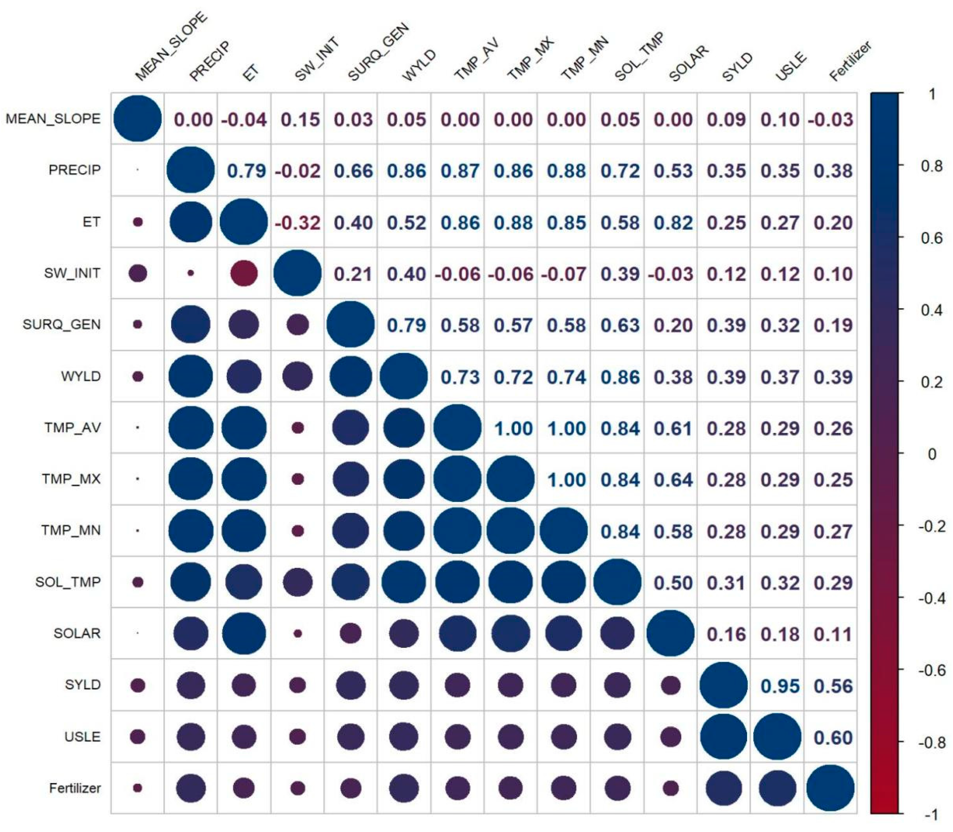
To eliminate the influence of multicollinearity [55,56,57], a correlation analysis was conducted on the pre-selected parameters, excluding the land use types since they are categorical variables. The results of the Pearson correlation analysis for the remaining 14 parameters are presented in Figure 6.
Based on the analysis of the relationships among the parameters, TN, and TP, parameters with a correlation greater than 0.75 were removed. Ultimately, 11 parameters were selected for the RF models, including four land use types, terrain slope, water yield, average temperature, fertilization, solar radiation, initial soil moisture, and sediment yield.
As land use type is a categorical variable, one-hot encoding was applied to convert it into binary variables, making them suitable for RF regression models and enhancing the model’s explanatory and predictive capabilities [58]. The Variance Inflation Factor (VIF) was then used to assess the degree of multicollinearity among these environmental factors. The results indicated that all selected parameters had VIF values below 10, confirming the absence of multicollinearity issues.

3.4. Variable Importance of the RF Model for TN and TP

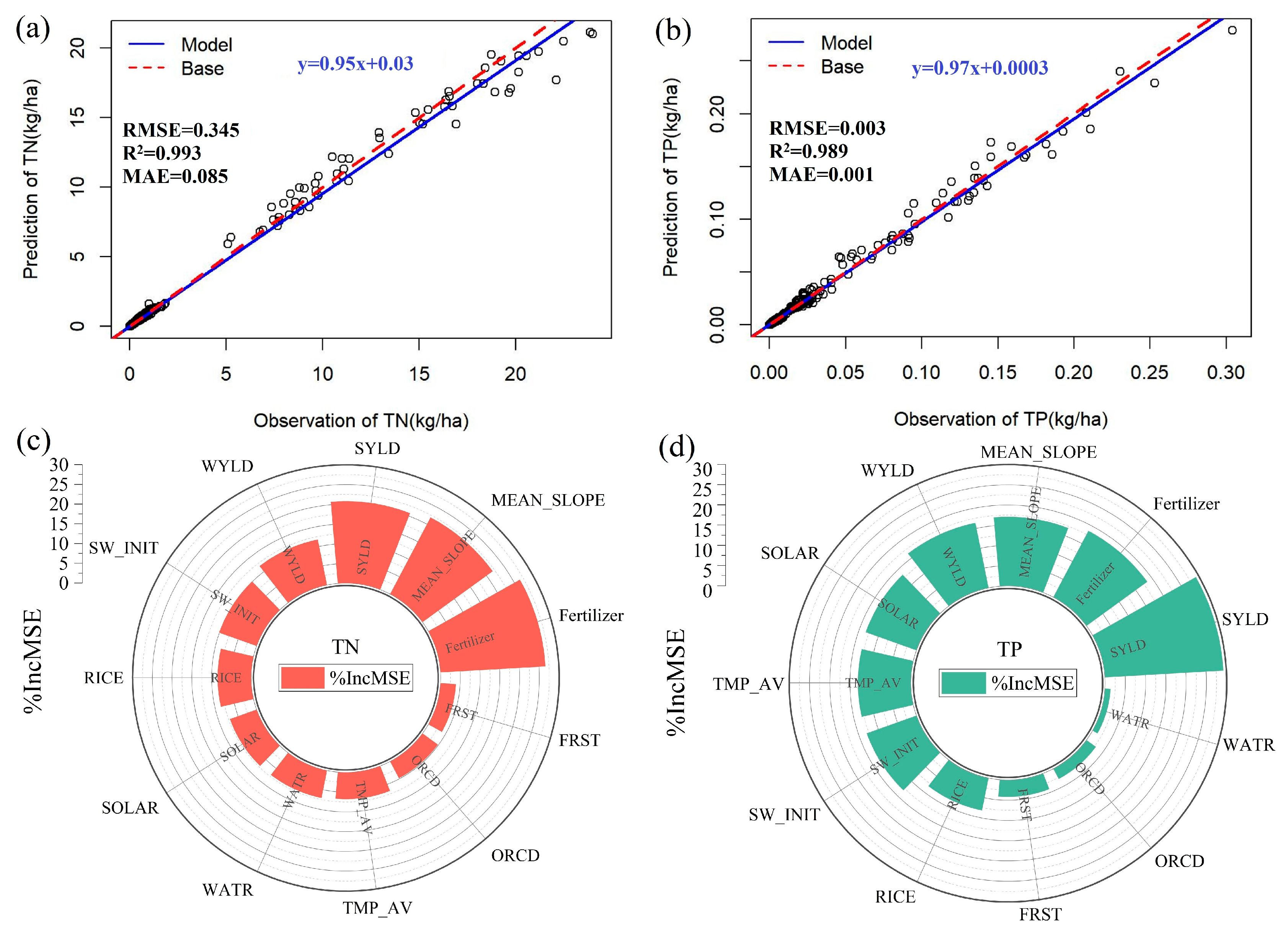
The constructed RF models for TN and TP exhibited excellent predictive accuracy and robust generalization ability. As shown in Figure 7a,b, there is a close linear relationship between the predicted and observed values. The RF model for TN achieved a root mean squared error (RMSE) of 0.345, a mean absolute error (MAE) of 0.085, and an R2 of 0.993. The RF model for TP achieved an RMSE of 0.003, an MAE of 0.001, and an R2 of 0.989. The RMSE and MAE values approaching 0 and R2 values being close to 1 indicate the strong performance of the models.
The importance of each variable was evaluated based on the change in mean squared error (MSE) of the model, with a higher percentage increase in MSE (%IncMSE) indicating a greater importance of the variable. As shown in Figure 7c, the %IncMSE were 26.57% for Fertilizer, 21.93% for MEAN_SLOPE, and 20.75% for SYLD, suggesting that fertilizer application, terrain slope, and sediment yield are key factors in nitrogen cycling and loss within each sub-watershed. For the RF model of TP (Figure 7d), the %IncMSE values were 29.26% for SYLD, 18.52% for Fertilizer, and 17.08% for MEAN_SLOPE, indicating that sediment yield is the most critical factor. The relatively lower importance of fertilization may be due to the smaller proportion of phosphorus in total fertilizers and the typically lower overall TP load.
Other factors, such as water yield, soil moisture, solar radiation, and temperature, significantly influence TN and TP loads indirectly by affecting soil conditions and erosion processes, which in turn impact the availability and transformation of nitrogen and phosphorus in the soil [59,60]. The average rainfall during June to August in the Baixi Reservoir Watershed accounts for 46.8% of the annual total. Furthermore, in this period, crops are in a rapid growth phase with peak nutrient demand, leading to maximum fertilizer application. The combination of heavy rainfall and fertilization activities causes significant changes in soil structure [61]. Under the erosive force of rainfall, freshly fertilized land becomes more prone to erosion and the soil becomes looser, greatly increasing the capacity of surface runoff to carry soil particles.
In the importance ranking of the RF models for TN and TP, cropland type emerged as the most critical factor among the different land use types, primarily due to human activities. Cropland exerts a substantial impact on TN and TP loads due to the high intensity of fertilization and frequent tillage, both of which can exacerbate soil erosion and nutrient loss [62,63]. In the Baixi Reservoir Watershed, the top 29% of HRUs that contribute the highest TN and TP loads are predominantly cropland, making these areas key sources of NPS pollution. Although cropland covers only 7.19% of the area, it accounts for 62.82% of the annual TN load and nearly half of the TP load. In contrast, forestland, which occupies 90.52% of the area, contributes 36.74% of the annual TN load and 55.32% of the annual TP load. The annual intensities of TN and TP loads are also highest in cropland; compared to forestland, the intensities of TN and TP loads in cropland are approximately 21 times and 10 times higher, respectively.

3.5. Impacts of Primary Controlling Factors on TN and TP

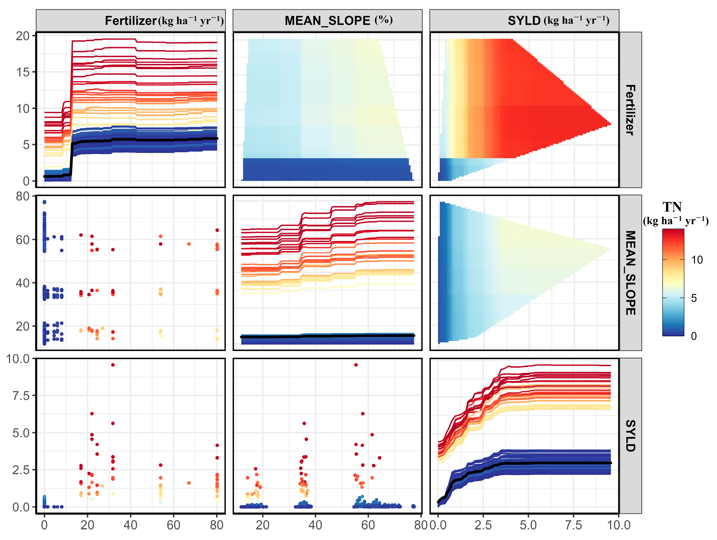
Since the %IncMSE values for fertilization, mean slope, and sediment yield exceeded 20% in the RF model for TN, and these variables were also the top three critical influencing factors in the RF model for TP, we conducted further analysis on their interactions. Partial dependency plots were generated for these factors based on the TN and TP Random Forest models to visualize and assess their combined effects.
In Figure 8 and Figure 9, the graphs on the diagonal display the univariate partial dependency plots and individual conditional expectation curves, the graphs above and to the right of this diagonal show the bivariate partial dependency plots, and the lower left presents scatter plots of the raw data for the variables. Here, high values of y are shown in dark red and low values in dark blue. Mid-range values are shown in yellow. To avoid interpreting the PDPs where there are no data (and hence potentially spurious H-statistics), extrapolated areas have been masked out by plotting the convex hull.
From the univariate partial dependency plots shown in Figure 8, fertilizer application (Fertilizer) has a significant positive effect on TN load. As fertilizer application increases, TN load per unit area also rises, with certain levels of fertilizer application exhibiting a pronounced leap effect [64]. For example, at a fertilizer application of 15 kg ha−1 yr−1, the intensity of TN load shows a substantial increase, with an approximate 400% rise. The mean slope of each hydrologic response unit is also positively correlated with TN load; as the mean slope increases, TN load per unit area correspondingly rises. Similarly, sediment yield (SYLD) is positively correlated with TN load, although the rate of increase in TN starts to decelerate once sediment yield reaches 3 kg ha−1 yr−1.
The interaction plots highlight a clear synergistic effect between sediment yield and fertilizer application on TN load. Specifically, when sediment yield exceeds 3 kg ha−1 yr−1 and fertilizer application exceeds 15 kg ha−1 yr−1, the intensity of TN load increases dramatically, surpassing 10 kg ha−1 yr−1. There are also synergistic effects observed between mean slope and fertilizer application, as well as between mean slope and sediment yield. When the slope percentage exceeds 46.63%, corresponding to slopes greater than 25°, and sediment yield exceeds 3 kg ha−1 yr−1, a significant increase in TN load per unit area is evident.
There is a positive correlation between sediment yield and TP load, without a distinct threshold (Figure 9). An increase in sediment yield indicates that more phosphorus-rich soil particles are being transported into the water, thereby raising the phosphorus concentration [65]. The mean slope is also positively correlated with TP load, as terrain slope significantly influences soil erosion, surface runoff, and pollutant transport [66,67]. Analysis of the impact of different slopes within cropland on nitrogen and phosphorus loads shows that slopes of 0–15° make up the largest proportion at 51.80%, slopes of 15–25° account for 39.26%, and slopes greater than 25° account for only 8.94%. However, from an intensity of load perspective, as the slope increases, the intensities of TN and TP loads also increase. For high-slope cropland (>25°), despite only covering 8.94% of the area, the intensities of TN and TP loads are 59.71 kg ha−1 yr−1 and 0.40 kg ha−1 yr−1, respectively, which are significantly higher than those of other slopes, aligning with the findings of the Random Forest model.
In the univariate partial dependency plots shown in Figure 9, TP load per unit area shows a sharp increase at a fertilizer application of 15 kg ha−1 yr−1 and peaks in the 30–40 kg ha−1 yr−1 range. Further analysis of the interaction between fertilizer application and sediment yield reveals that the effect of fertilizer application on TP load per unit area is particularly pronounced at sediment yields below 3 kg ha−1 yr−1. This is because lower sediment yields indicate minimal soil erosion, making fertilizer application the dominant factor. When fertilizer application reaches the range from 30 to 40 kg ha−1 yr−1, increasing sediment yield continues to transport phosphorus into the water, resulting in TP load per unit area exceeding 0.15 kg ha−1 yr−1. When fertilizer application continues to increase beyond 40 kg ha−1 yr−1, the corresponding sediment yield is below 4 kg ha−1 yr−1, so even with increased fertilizer application, phosphorus cannot be transported into the water via sediment. During June to August, the sediment across the whole watershed constitutes 70.19% of the annual total, as indicated by the temporal distribution characteristics of NPS. These soil particles contain not only organic matter but also excess fertilizer components, particularly nitrogen and phosphorus. As sediment yield increases, more nitrogen and phosphorus are washed into the water, resulting in a sharp rise in TN and TP loads per unit area [68]. Therefore, reducing fertilizer application and implementing soil and water conservation measures are essential for mitigating NPS pollution.
The interaction between slope and fertilizer application is relatively weak, mainly because fertilization practices do not take slope into account but rather focus on whether the land is used for cropland. As previously analyzed, cropland is distributed across various slopes, so the correlation between fertilizer application and slope is not significant.

4. Conclusions

This study presents a novel approach that integrates the SWAT model with the Random Forest algorithm to effectively identify the key factors influencing NPS pollution. Applied to the Baixi Reservoir Watershed, this approach enabled a comprehensive analysis of the interactions among these factors. The validation results for both the SWAT and Random Forest models demonstrate the robustness and suitability of this method for the watershed, confirming its effectiveness in accurately capturing the dynamics of NPS pollution in the region.
The results further reveal significant seasonal variations in sediment yield, water yield, TP load, and TN load by validated SWAT for the Baixi Reservoir Watershed. The average values of CV were 1.28 for sediment yield, 1.40 for TP load, and 1.03 for TN load, indicating highly uneven distribution throughout the year. Spatially, areas with high nitrogen and phosphorus loads were primarily concentrated in sub-watersheds with cropland. The Random Forest analysis of key factors indicates that fertilizer application, sediment yield, and terrain slope are the primary controlling factors for TN and TP loads. When fertilizer application and sediment yield exceed 15 kg ha−1 yr−1 and 3 kg ha−1 yr−1, respectively, their synergistic effect leads to a sharp increase in the load per unit area of nitrogen and phosphorus, with TN exceeding 10 kg ha−1 yr−1 and TP exceeding 0.15 kg ha−1 yr−1. Therefore, the Baixi Reservoir Management should prioritize reducing sediment loads within the watershed by limiting fertilizer application and adopting effective water and soil conservation practices. Particular attention should be given to sediment generation in sub-watersheds 2, 5, 10, 16, and 17 during the months of June to August, with proactive prevention and control measures implemented accordingly.
It is worth noting that the thresholds for correlation analysis and parameter selection in this study were primarily informed by previous research. Given that the input parameters are pivotal to the overall performance of the SWAT and machine learning model, further exploration and analysis of more effective parameter selection approaches are necessary. Additionally, the key factors influencing NPS pollution may vary due to the unique geographical, ecological, and socio-economic characteristics of different watersheds. Nonetheless, the analytical framework and methodology proposed in this paper exhibit a degree of general applicability. Using this approach to analyze the key factors controlling NPS pollution from a watershed perspective enables more effective implementation of management strategies.

Supplementary Materials

The following supporting information can be downloaded at: https://www.mdpi.com/article/10.3390/w16213026/s1, Table S1: Description of 26 key parameters and fitted value in SWAT-CUP.; Table S2: Monthly values of the 11 selected parameters and TN/TP loads for different watersheds; Table S3. The results of five-fold cross-validation for TP/TN RF model. Figure S1: Error & Trees for (a) TP and (b) TN RF model.

Author Contributions

Conceptualization, M.Y., Z.W. and Q.Z.; methodology, M.Y. and Z.W.; software, M.Y.; validation, M.Y., Z.W., Q.Z., Y.S. and Q.J.; formal analysis, M.Y., Q.Z. and Q.H.; investigation, Z.W., Q.Z. and Q.H.; visualization, M.Y., Z.W., Q.J. and K.W.; writing—original draft, M.Y.; data curation, Q.Z., Y.S., X.W., K.W. and J.C.; writing—review and editing, M.Y., Z.W., Q.Z., X.W. and J.C.; project administration, Z.W., Q.Z. and K.W. All authors have read and agreed to the published version of the manuscript.

Funding

This research was supported by the Joint Funds of the Zhejiang Provincial Natural Science Foundation of China under Grant No. LZJWY23E090007 and the K.C. Wong Magna Fund of Ningbo University. It was funded by Baixi Reservoir Management Bureau, grant number NBITC-202330424BX.

Data Availability Statement

The data that support the findings of this study are available from the corresponding author, upon reasonable request.

Conflicts of Interest

The authors declare no conflicts of interest.

References

  1. Bai, X.; Shen, W.; Wang, P.; Chen, X.; He, Y. Response of Non-Point Source Pollution Loads to Land Use Change under Different Precipitation Scenarios from a Future Perspective. Water Resour. Manag. 2020, 34, 3987–4002. [Google Scholar] [CrossRef]
  2. Wang, H.; Bouwman, A.F.; Van Gils, J.; Vilmin, L.; Beusen, A.H.W.; Wang, J.; Liu, X.; Yu, Z.; Ran, X. Hindcasting Harmful Algal Bloom Risk Due to Land-Based Nutrient Pollution in the Eastern Chinese Coastal Seas. Water Res. 2023, 231, 119669. [Google Scholar] [CrossRef] [PubMed]
  3. Fianko, J.R.; Korankye, M.B. Quality Characteristics of Water Used for Irrigation in Urban and Peri-Urban Agriculture in Greater Accra Region of Ghana: Health and Environmental Risk. West Afr. J. Appl. Ecol. 2020, 28, 131–143. [Google Scholar]
  4. Nielsen, M.C. The Effects of Recreational Water Exposure on Human Skin: Toxin Penetration and Microbiome Alteration. Ph.D. Thesis, University of California, Irvine, CA, USA, 2020. [Google Scholar]
  5. Mohammed, V.; Arockiaraj, J. Unveiling the Trifecta of Cyanobacterial Quorum Sensing: LuxI, LuxR and LuxS as the Intricate Machinery for Harmful Algal Bloom Formation in Freshwater Ecosystems. Sci. Total Environ. 2024, 924, 171644. [Google Scholar] [CrossRef]
  6. Li, H.; Chen, Q.; Liu, G.; Lombardi, G.V.; Su, M.; Yang, Z. Uncovering the Risk Spillover of Agricultural Water Scarcity by Simultaneously Considering Water Quality and Quantity. J. Environ. Manag. 2023, 343, 118209. [Google Scholar] [CrossRef]
  7. Zhang, J.L.; Li, Y.P.; Wang, C.X.; Huang, G.H. An Inexact Simulation-Based Stochastic Optimization Method for Identifying Effluent Trading Strategies of Agricultural Nonpoint Sources. Agric. Water Manag. 2015, 152, 72–90. [Google Scholar] [CrossRef]
  8. Fleming, P.M.; Stephenson, K.; Collick, A.S.; Easton, Z.M. Targeting for Nonpoint Source Pollution Reduction: A Synthesis of Lessons Learned, Remaining Challenges, and Emerging Opportunities. J. Environ. Manag. 2022, 308, 114649. [Google Scholar] [CrossRef]
  9. Li, Q.; Ouyang, W.; Zhu, J.; Lin, C.; He, M. Discharge Dynamics of Agricultural Diffuse Pollution under Different Rainfall Patterns in the Middle Yangtze River. J. Environ. Manag. 2023, 347, 119116. [Google Scholar] [CrossRef]
  10. Zhang, C.; Gao, X.; Wang, L.; Chen, Y. Analysis of Agricultural Pollution by Flood Flow Impact on Water Quality in a Reservoir Using a Three-Dimensional Water Quality Model. J. Hydroinform. 2013, 15, 1061–1072. [Google Scholar] [CrossRef]
  11. Sedláček, J.; Bábek, O.; Nováková, T. Sedimentary Record and Anthropogenic Pollution of a Complex, Multiple Source Fed Dam Reservoirs: An Example from the Nové Mlýny Reservoir, Czech Republic. Sci. Total Environ. 2017, 574, 1456–1471. [Google Scholar] [CrossRef]
  12. Zhao, X.; Gao, B.; Xu, D.; Gao, L.; Yin, S. Heavy Metal Pollution in Sediments of the Largest Reservoir (Three Gorges Reservoir) in China: A Review. Environ. Sci. Pollut. Res. 2017, 24, 20844–20858. [Google Scholar] [CrossRef]
  13. Xu, W.; Liu, L.; Zhu, S.; Sun, A.; Wang, H.; Ding, Z. Identifying the Critical Areas and Primary Sources for Agricultural Non-Point Source Pollution Management of an Emigrant Town within the Three Gorges Reservoir Area. Environ. Monit. Assess. 2023, 195, 602. [Google Scholar] [CrossRef] [PubMed]
  14. Zhou, J.; Liu, X.; Liu, X.; Wang, W.; Wang, L. Assessing Agricultural Non-Point Source Pollution Loads in Typical Basins of Upper Yellow River by Incorporating Critical Impacting Factors. Process Saf. Environ. Prot. 2023, 177, 17–28. [Google Scholar] [CrossRef]
  15. Ding, L.; Qi, C.; Zhang, W. Distribution Characteristics of Non-Point Source Pollution of TP and Identification of Key Source Areas in Nanyi Lake (China) Basin: Based on InVEST Model and Source List Method. Environ. Sci. Pollut. Res. 2023, 30, 117464–117484. [Google Scholar] [CrossRef] [PubMed]
  16. Ding, X.; Liu, L. Long-Term Effects of Anthropogenic Factors on Nonpoint Source Pollution in the Upper Reaches of the Yangtze River. Sustainability 2019, 11, 2246. [Google Scholar] [CrossRef]
  17. Deshmukh, D.S.; Chaube, U.C.; Ekube Hailu, A.; Aberra Gudeta, D.; Tegene Kassa, M. Estimation and Comparision of Curve Numbers Based on Dynamic Land Use Land Cover Change, Observed Rainfall-Runoff Data and Land Slope. J. Hydrol. 2013, 492, 89–101. [Google Scholar] [CrossRef]
  18. Wang, H.; Wu, Z.; Hu, C. A Comprehensive Study of the Effect of Input Data on Hydrology and Non-Point Source Pollution Modeling. Water Resour. Manag. 2015, 29, 1505–1521. [Google Scholar] [CrossRef]
  19. Breiman, L. Random Forests. Mach. Learn. 2001, 45, 5–32. [Google Scholar] [CrossRef]
  20. He, S.; Wu, J.; Wang, D.; He, X. Predictive Modeling of Groundwater Nitrate Pollution and Evaluating Its Main Impact Factors Using Random Forest. Chemosphere 2022, 290, 133388. [Google Scholar] [CrossRef]
  21. Amare, S.; Langendoen, E.; Keesstra, S.; Ploeg, M.v.d.; Gelagay, H.; Lemma, H.; van der Zee, S.E.A.T.M. Susceptibility to Gully Erosion: Applying Random Forest (RF) and Frequency Ratio (FR) Approaches to a Small Catchment in Ethiopia. Water 2021, 13, 216. [Google Scholar] [CrossRef]
  22. Avand, M.; Mohammadi, M.; Mirchooli, F.; Kavian, A.; Tiefenbacher, J.P. A New Approach for Smart Soil Erosion Modeling: Integration of Empirical and Machine-Learning Models. Environ. Model. Assess. 2023, 28, 145–160. [Google Scholar] [CrossRef]
  23. Liu, Y.; Heuvelink, G.B.M.; Bai, Z.; He, P.; Jiang, R.; Huang, S.; Xu, X. Statistical Analysis of Nitrogen Use Efficiency in Northeast China Using Multiple Linear Regression and Random Forest. J. Integr. Agric. 2022, 21, 3637–3657. [Google Scholar] [CrossRef]
  24. Krysanova, V.; White, M. Advances in Water Resources Assessment with SWAT—An Overview. Hydrol. Sci. J. 2015, 60, 771–783. [Google Scholar] [CrossRef]
  25. Hanief, A.; Laursen, A.E. Meeting Updated Phosphorus Reduction Goals by Applying Best Management Practices in the Grand River Watershed, Southern Ontario. Ecol. Eng. 2019, 130, 169–175. [Google Scholar] [CrossRef]
  26. Cao, Y.; Fu, C.; Wang, X.; Dong, L.; Yao, S.; Xue, B.; Wu, H.; Wu, H. Decoding the Dramatic Hundred-Year Water Level Variations of a Typical Great Lake in Semi-Arid Region of Northeastern Asia. Sci. Total Environ. 2021, 770, 145353. [Google Scholar] [CrossRef]
  27. Schmalz, B.; Kuemmerlen, M.; Kiesel, J.; Cai, Q.; Jähnig, S.C.; Fohrer, N. Impacts of Land Use Changes on Hydrological Components and Macroinvertebrate Distributions in the Poyang Lake Area. Ecohydrology 2015, 8, 1119–1136. [Google Scholar] [CrossRef]
  28. Xiao, H.; Ji, W. Relating Landscape Characteristics to Non-Point Source Pollution in Mine Waste-Located Watersheds Using Geospatial Techniques. J. Environ. Manag. 2007, 82, 111–119. [Google Scholar] [CrossRef]
  29. Kuemmerlen, M.; Schmalz, B.; Cai, Q.; Haase, P.; Fohrer, N.; Jähnig, S.C. An Attack on Two Fronts: Predicting How Changes in Land Use and Climate Affect the Distribution of Stream Macroinvertebrates. Freshw. Biol. 2015, 60, 1443–1458. [Google Scholar] [CrossRef]
  30. Woo, S.Y.; Jung, C.G.; Lee, J.W.; Kim, S.J. Evaluation of Watershed Scale Aquatic Ecosystem Health by SWAT Modeling and Random Forest Technique. Sustainability 2019, 11, 3397. [Google Scholar] [CrossRef]
  31. Matomela, N.; Li, T.; Zhang, P.; Ikhumhen, H.O.; Lopes, N.D.R. Role of Landscape and Land-Use Transformation on Nonpoint Source Pollution and Runoff Distribution in the Dongsheng Basin, China. Sustainability 2023, 15, 8325. [Google Scholar] [CrossRef]
  32. Shi, J.; Jin, R.; Zhu, W. Quantification of Effects of Natural Geographical Factors and Landscape Patterns on Non-Point Source Pollution in Watershed Based on Geodetector: Burhatong River Basin, Northeast China as An Example. Chin. Geogr. Sci. 2022, 32, 707–723. [Google Scholar] [CrossRef]
  33. Chen, L.; Liu, R.M.; Huang, Q.; Chen, Y.X.; Gao, S.H.; Sun, C.C.; Shen, Z.Y.; Ou, S.Z.; Chen, S.L. An Integrated Simulation-Monitoring Framework for Nitrogen Assessment: A Case Study in the Baixi Watershed, China. Procedia Environ. Sci. 2012, 13, 1076–1090. [Google Scholar] [CrossRef]
  34. Tan, M.L.; Ficklin, D.L.; Dixon, B.; Yusop, Z.; Chaplot, V. Impacts of DEM Resolution, Source, and Resampling Technique on SWAT-Simulated Streamflow. Appl. Geogr. 2015, 63, 357–368. [Google Scholar] [CrossRef]
  35. Zhang, X.; Cao, W.; Guo, Q.; Wu, S. Effects of Landuse Change on Surface Runoff and Sediment Yield at Different Watershed Scales on the Loess Plateau. Int. J. Sediment Res. 2010, 25, 283–293. [Google Scholar] [CrossRef]
  36. Soriano, M.C.H. Soil Processes and Current Trends in Quality Assessment; BoD—Books on Demand; Intechopen: London, UK, 2013; ISBN 978-953-51-1029-3. [Google Scholar]
  37. Aouissi, J.; Benabdallah, S.; Chabaâne, Z.L.; Cudennec, C. Evaluation of Potential Evapotranspiration Assessment Methods for Hydrological Modelling with SWAT—Application in Data-Scarce Rural Tunisia. Agric. Water Manag. 2016, 174, 39–51. [Google Scholar] [CrossRef]
  38. Abbaspour, K.C.; Yang, J.; Maximov, I.; Siber, R.; Bogner, K.; Mieleitner, J.; Zobrist, J.; Srinivasan, R. Modelling Hydrology and Water Quality in the Pre-Alpine/Alpine Thur Watershed Using SWAT. J. Hydrol. 2007, 333, 413–430. [Google Scholar] [CrossRef]
  39. Dong, G.; Hu, Z.; Liu, X.; Fu, Y.; Zhang, W. Spatio-Temporal Variation of Total Nitrogen and Ammonia Nitrogen in the Water Source of the Middle Route of the South-To-North Water Diversion Project. Water 2020, 12, 2615. [Google Scholar] [CrossRef]
  40. Smith, L.E.; Siciliano, G. A Comprehensive Review of Constraints to Improved Management of Fertilizers in China and Mitigation of Diffuse Water Pollution from Agriculture. Agric. Ecosyst. Environ. 2015, 209, 15–25. [Google Scholar] [CrossRef]
  41. Arnold, J.G.; Moriasi, D.N.; Gassman, P.W.; Abbaspour, K.C.; White, M.J.; Srinivasan, R.; Santhi, C.; Harmel, R.D.; Griensven, A.V.; Liew, M.W.V.; et al. SWAT: Model Use, Calibration, and Validation. Trans. ASABE 2012, 55, 1491–1508. [Google Scholar] [CrossRef]
  42. Malik, M.A.; Dar, A.Q.; Jain, M.K. Modelling Streamflow Using the SWAT Model and Multi-Site Calibration Utilizing SUFI-2 of SWAT-CUP Model for High Altitude Catchments, NW Himalaya’s. Model. Earth Syst. Environ. 2022, 8, 1203–1213. [Google Scholar] [CrossRef]
  43. Huiyong, W.; Chaopu, T.; Liangjie, W.; Lei, D.; Yongqiu, X.; Xiaoyuan, Y. Spatiotemporal Distribution Characteristics and Key Sources of Nitrogen Pollution in a Typical Agricultural Watershed Based on SWAT Model. J. Lake Sci. 2022, 34, 517–527. [Google Scholar] [CrossRef]
  44. Huang, H.; Jia, R.; Shi, X.; Liang, J.; Dang, J. Feature Selection and Hyper Parameters Optimization for Short-Term Wind Power Forecast. Appl. Intell. 2021, 51, 6752–6770. [Google Scholar] [CrossRef]
  45. Cibin, R.; Sudheer, K.P.; Chaubey, I. Sensitivity and Identifiability of Stream Flow Generation Parameters of the SWAT Model. Hydrol. Process. 2010, 24, 1133–1148. [Google Scholar] [CrossRef]
  46. Liu, R.; Xu, F.; Zhang, P.; Yu, W.; Men, C. Identifying Non-Point Source Critical Source Areas Based on Multi-Factors at a Basin Scale with SWAT. J. Hydrol. 2016, 533, 379–388. [Google Scholar] [CrossRef]
  47. Rostamian, R.; Jaleh, A.; Majid, A.; Mousavi, S.-F.; Heidarpour, M.; Jalalian, A.; Mikayilov, F. Application of a SWAT Model for Estimating Runoff and Sediment in Two Mountainous Basins in Central Iran. Hydrol. Sci. J. 2008, 53, 977–988. [Google Scholar] [CrossRef]
  48. Park, J.; Lee, W.H.; Kim, K.T.; Park, C.Y.; Lee, S.; Heo, T.-Y. Interpretation of Ensemble Learning to Predict Water Quality Using Explainable Artificial Intelligence. Sci. Total Environ. 2022, 832, 155070. [Google Scholar] [CrossRef]
  49. Inglis, A.; Parnell, A.; Hurley, C.B. Visualizing Variable Importance and Variable Interaction Effects in Machine Learning Models. J. Comput. Graph. Stat. 2022, 31, 766–778. [Google Scholar] [CrossRef]
  50. Gao, P.; Josefson, M. Temporal Variations of Suspended Sediment Transport in Oneida Creek Watershed, Central New York. J. Hydrol. 2012, 426–427, 17–27. [Google Scholar] [CrossRef]
  51. Siedt, M.; Schäffer, A.; Smith, K.E.C.; Nabel, M.; Roß-Nickoll, M.; van Dongen, J.T. Comparing Straw, Compost, and Biochar Regarding Their Suitability as Agricultural Soil Amendments to Affect Soil Structure, Nutrient Leaching, Microbial Communities, and the Fate of Pesticides. Sci. Total Environ. 2021, 751, 141607. [Google Scholar] [CrossRef]
  52. Parajuli, P.B.; Nelson, N.O.; Frees, L.D.; Mankin, K.R. Comparison of AnnAGNPS and SWAT Model Simulation Results in USDA-CEAP Agricultural Watersheds in South-Central Kansas. Hydrol. Process. 2009, 23, 748–763. [Google Scholar] [CrossRef]
  53. Ongley, E.D.; Xiaolan, Z.; Tao, Y. Current Status of Agricultural and Rural Non-Point Source Pollution Assessment in China. Environ. Pollut. 2010, 158, 1159–1168. [Google Scholar] [CrossRef] [PubMed]
  54. Nobre, R.L.; Caliman, A.; Cabral, C.R.; de Carvalho Araújo, F.; Guerin, J.; Dantas, F.D.; Quesado, L.B.; Venticinque, E.M.; Guariento, R.D.; Amado, A.M.; et al. Precipitation, Landscape Properties and Land Use Interactively Affect Water Quality of Tropical Freshwaters. Sci. Total Environ. 2020, 716, 137044. [Google Scholar] [CrossRef] [PubMed]
  55. Schroeder, M.A.; Lander, J.; Levine-Silverman, S. Diagnosing and Dealing with Multicollinearity. West. J. Nurs. Res. 1990, 12, 175–187. [Google Scholar] [CrossRef] [PubMed]
  56. Alin, A. Multicollinearity. WIREs Comput. Stat. 2010, 2, 370–374. [Google Scholar] [CrossRef]
  57. Kim, J.H. Multicollinearity and Misleading Statistical Results. Korean J. Anesthesiol. 2019, 72, 558–569. [Google Scholar] [CrossRef]
  58. Dahouda, M.K.; Joe, I. A Deep-Learned Embedding Technique for Categorical Features Encoding. IEEE Access 2021, 9, 114381–114391. [Google Scholar] [CrossRef]
  59. Tang, L.; Yang, D.; Hu, H.; Gao, B. Detecting the Effect of Land-Use Change on Streamflow, Sediment and Nutrient Losses by Distributed Hydrological Simulation. J. Hydrol. 2011, 409, 172–182. [Google Scholar] [CrossRef]
  60. Williams, M.R.; Penn, C.J.; King, K.W.; McAfee, S.J. Surface-to-Tile Drain Connectivity and Phosphorus Transport: Effect of Antecedent Soil Moisture. Hydrol. Process. 2023, 37, e14831. [Google Scholar] [CrossRef]
  61. Wang, Z.; Yue, F.; Wang, Y.; Qin, C.; Ding, H.; Xue, L.-L.; Li, S. The Effect of Heavy Rainfall Events on Nitrogen Patterns in Agricultural Surface and Underground Streams and the Implications for Karst Water Quality Protection. Agric. Water Manag. 2022, 266, 107600. [Google Scholar] [CrossRef]
  62. Su, L.; Huang, D.; Zhou, L. Differences in Sediment Provenance from Rainfall and Snowmelt Erosion in the Mollisol Region of Northeast China. Earth Surf. Process. Landf. 2024, 49, 2442–2457. [Google Scholar] [CrossRef]
  63. Wu, J.; Lu, J. Landscape Patterns Regulate Non-Point Source Nutrient Pollution in an Agricultural Watershed. Sci. Total Environ. 2019, 669, 377–388. [Google Scholar] [CrossRef] [PubMed]
  64. Xiao, M.; Li, Y.; Jia, Y.; Wang, J. Effect on Water Consumption and Non-Point Source Pollutants Loss under Different Water and Nitrogen Regulation of Paddy Field in Southern China. Pol. J. Environ. Stud. 2022, 31, 1389–1398. [Google Scholar] [CrossRef] [PubMed]
  65. Ni, J.; Wei, C.; Xie, D. GIS-Based Prediction of Nutrient Loss from a Small Watershed. ACTA Pedol. Sin. 2013, 41, 837–844. [Google Scholar]
  66. Panuska, J.C.; Moore, I.D.; Kramer, L.A. Terrain Analysis: Integration into the Agricultural Nonpoint Source (AGNPS) Pollution Model. J. Soil Water Conserv. 1991, 46, 59–64. [Google Scholar]
  67. Lowe, M.A.; McGrath, G.; Leopold, M. The Impact of Soil Water Repellency and Slope upon Runoff and Erosion. Soil Tillage Res. 2021, 205, 104756. [Google Scholar] [CrossRef]
  68. Osterholz, W.; Simpson, Z.; Williams, M.; Shedekar, V.; Penn, C.; King, K. New Phosphorus Losses via Tile Drainage Depend on Fertilizer Form, Placement, and Timing. J. Environ. Qual. 2024, 53, 241–252. [Google Scholar] [CrossRef]
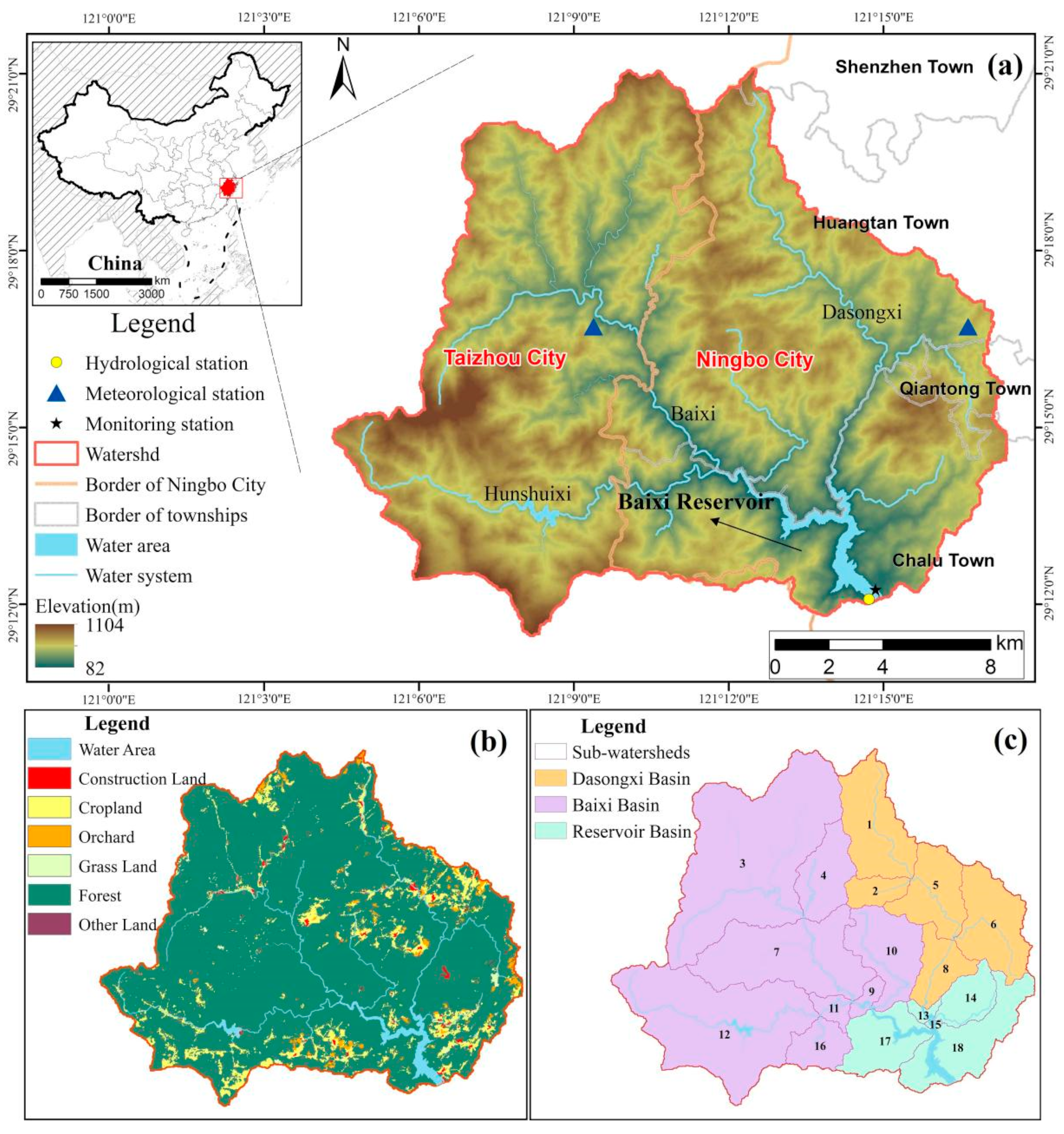
Figure 1. (a) Geographic location of Baixi Reservoir, two meteorological stations, and one hydrological station, and distribution of rivers within the watershed; (b) spatial distribution of land use types; (c) the whole watershed divided into three smaller basins, and the distribution of 18 sub-watersheds.
Water 16 03026 g001
Figure 2. Process of importance analysis for RF factors.
Water 16 03026 g002
Figure 3. Calibration and validation results of monthly (a) flow discharge, (b) NH3-N, (c) TP, and (d) TN in the Baixi Reservoir Watershed. The dashed line divides the calibration period and validation period.
Water 16 03026 g003
Figure 4. The variation of monthly (a) sediment yield, (b) water yield, (c) TP load, and (d) TN load; (e) the coefficient of variation and (f) the absolute change rate.
Water 16 03026 g004
Figure 5. Distribution of average annual intensities of (a) TN and (b) TP loads across 18 sub-watersheds in the Baixi Reservoir Watershed.
Water 16 03026 g005
Figure 6. Pearson correlation coefficients for 14 pre-selected parameters. The size of the circle represents the magnitude of the correlation.
Water 16 03026 g006
Figure 7. Comparison of the observations and predictions made by the RF model for (a) TN and (b) TP; RF variable importance of (c) TN and (d) TP.
Water 16 03026 g007
Figure 8. Generalized PDPs for the primary controlling factors of TN.
Water 16 03026 g008
Figure 9. Generalized PDPs for the primary controlling factors of TP.
Water 16 03026 g009
Table 1. SWAT Modeling Data and Sources.
Data CategoryDescriptionPrecisionSource
DEMProvides elevation and slope data, crucial for simulating runoff, flow direction, and watershed boundaries [34].90 mhttp://srtm.csi.cgiar.org/ (accessed on 8 October 2022)
Land UseDescribes land utilization (e.g., forest, agriculture), critical for estimating runoff and sediment yield [35].1:100,000Ningbo Municipal Bureau of Land and Resources
SoilIncludes texture, organic matter, and hydraulic properties, key for water retention and nutrient cycling [36].1:1,000,000Nanjing Institute of Soil Science
MeteorologyWeather data (e.g., precipitation, temperature) affects processes like runoff and evapotranspiration [37].Daily AverageNingbo Meteorological Bureau
HydrologyStreamflow and groundwater data for calibrating and validating model predictions [38].Daily AverageBaixi Reservoir Management Bureau, Ningbo
TN, TP, NH3-NThese nutrients are key indicators of water pollution, particularly in relation to agricultural runoff and waste management [39]. Monthly AverageNingbo Ecology and Environment Bureau, Ninghai Branch
FertilizerFertilizer application data are used to simulate nitrogen and phosphorus runoff, impacting water quality [40]./Ninghai Statistical Yearbook, Field Surveys
Table 2. Comprehensive Sensitivity Rankings of 26 Key Parameters and Fitted Values in SWAT-CUP.
CategoryParameter NameRangeFitted ValueSensitivity Rank
MinMax
Vegetation and ManagementFRT_SURFACE010.496
BIOMIX010.425
SoilSOL_NO3(1)010022.081
SOL_ORGN(1)018001357.253
SOL_K(1)020001158.1911
SOL_ORGP(1)0600345.9512
SOL_BD(1)0.92.51.1416
SOL_Z(1)0800385.9620
SOL_AWC(1)010.4726
Nutrient TransportPHOSKD100200198.344
NPERCO010.358
PPERCO1017.515.439
Hydrological ProcessESCO010.0214
SURLAG0.05246.8615
CN2359866.9419
GroundwaterALPHA_BF010.222
REVAPMN0500352.635
GW_DELAY050022.57
GW_REVAP0.020.20.1810
GWQMN050001310.3613
RCHRG_DP010.1318
Channel and ErosionCH_K2−0.01500235.7117
USLE_P010.3921
CH_N2−0.010.30.1622
ERORGN053.5723
ERORGP050.0324
Disclaimer/Publisher’s Note: The statements, opinions and data contained in all publications are solely those of the individual author(s) and contributor(s) and not of MDPI and/or the editor(s). MDPI and/or the editor(s) disclaim responsibility for any injury to people or property resulting from any ideas, methods, instructions or products referred to in the content.