Landslide Deformation Analysis and Prediction with a VMD-SA-LSTM Combined Model

Abstract

The evolution of landslides is influenced by the complex interplay of internal geological factors and external triggering factors, resulting in nonlinear dynamic changes. Although deep learning methods have demonstrated advantages in predicting multivariate landslide displacement, their performance is often constrained by the challenges of extracting intricate features from extended time-series data. To address this challenge, we propose a novel displacement prediction model that integrates Variational Mode Decomposition (VMD), Self-Attention (SA), and Long Short-Term Memory (LSTM) networks. The model first employs VMD to decompose cumulative landslide displacement into trend, periodic, and stochastic components, followed by an assessment of the correlation between these components and the triggering factors using grey relational analysis. Subsequently, the self-attention mechanism is incorporated into the LSTM model to enhance its ability to capture complex dependencies. Finally, each displacement component is fed into the SA-LSTM model for separate predictions, which are then reconstructed to obtain the cumulative displacement prediction. Using the Zhonghai Village tunnel entrance (ZVTE) landslide as a case study, we validated the model with displacement data from GPS point 105 and made predictions for GPS point 104 to evaluate the model’s generalization capability. The results indicated that the RMSE and MAPE for SA-LSTM, LSTM, and TCN-LSTM at GPS point 105 were 0.3251 and 1.6785, 0.6248 and 2.9130, and 1.1777 and 5.5131, respectively. These findings demonstrate that SA-LSTM outperformed the other models in terms of complex feature extraction and accuracy. Furthermore, the RMSE and MAPE at GPS point 104 were 0.4232 and 1.0387, further corroborating the model’s strong extrapolation capability and its effectiveness in landslide monitoring.

1. Introduction

Landslides are a globally prevalent natural disaster, and in recent decades, such events have occurred with increasing frequency worldwide, resulting in significant annual losses of life and property [1,2]. This risk is especially pronounced in regions with fragile geological conditions, where external triggers, such as earthquakes and heavy rainfall, heighten the likelihood of landslides, posing severe threats to the safety of local residents and infrastructure [3,4,5]. Landslide prediction and forecasting are critical strategies for mitigating landslide disasters. Accurate predictions provide timely warning signals to individuals in danger zones, thereby reducing or preventing casualties. Furthermore, effective predictions of landslides that may disrupt transportation infrastructure, such as roads, bridges, and tunnels, enable traffic management authorities to proactively inspect and maintain hazardous areas, thus averting catastrophic consequences. Additionally, precise landslide predictions furnish emergency management authorities with a scientific basis for making rescue decisions and organizing response efforts, ensuring the effectiveness and safety of rescue operations. During a landslide’s progression, displacement and deformation clearly reflect instability trends. Research focused on predicting landslide displacement aids in analyzing future trends, thereby enhancing disaster prevention and mitigation capabilities. Consequently, establishing an effective landslide deformation prediction model is essential for analyzing deformation characteristics, forecasting future trends, and minimizing the risks associated with landslides [6,7,8,9].

The evolution of landslide displacement is inherently complex, driven by the long-term interplay between internal geological and hydrological conditions and external inducing factors such as rainfall and seismic activity. This interaction results in nonlinear and dynamic changes in displacement [10,11,12]. Methods based on physical and data-driven approaches represent the two primary means of predicting landslide displacement. Physical models integrate geomechanical properties, hydraulic response mechanisms, and other relevant physical characteristics to forecast landslide behaviour. However, these models necessitate accurate parameter inputs and complex assumptions, which can result in inadequate performance when addressing the nonlinear dynamic changes associated with landslides, thereby limiting their applicability in rapidly changing environments [13,14]. In contrast, data-driven models are receiving increasing attention due to their superior accuracy, lower experimental costs, and broad applicability [15]. These models can swiftly respond to dynamically changing monitoring data, providing real-time predictions that enhance their suitability and flexibility in practical applications.

In recent years, the integration of artificial intelligence with time-series decomposition theory, which accounts for external factors influencing landslide displacement, has garnered significant attention from researchers focusing on coupled prediction models. These models utilize time-series decomposition techniques to decompose cumulative landslide displacement into distinct components with physical significance, establishing predictive models for analyzing these components across various frequencies [16]. This approach not only reduces the complexity of displacement data but also effectively enhances prediction accuracy. Traditional time-series decomposition methods include mathematical approaches [17,18,19,20], wavelet analysis [21], and Empirical Mode Decomposition (EMD) [22,23]. Techniques such as the moving average [17,18,19] and mean exponential smoothing [20,24] decompose landslide cumulative displacement into trend and periodic components. While these methods are relatively straightforward and yield components with clear physical meanings, they often overlook random variations caused by external factors, such as non-seasonal rainfall. Wavelet analysis and Empirical Mode Decomposition offer more refined approaches by partitioning landslide displacement, which exhibits nonlinear dynamics, into components with distinct characteristics. Ren et al. [21] employed wavelet analysis to decompose the surface displacement of the Shuping landslide in the Three Gorges Area into components with specific time-frequency attributes. Similarly, Shihabudheen et al. [23] utilized Empirical Mode Decomposition (EMD) to decompose landslide displacement series into intrinsic mode functions (IMFs) that capture local features, along with a residual component. However, wavelet analysis may face challenges in selecting an appropriate wavelet basis function, and Empirical Mode Decomposition is susceptible to issues such as endpoint effects and mode mixing, which can obscure the physical significance of the decomposed components. Recently, Dragomiretskiy et al. [25] introduced the adaptive and fully recursive Variational Mode Decomposition (VMD) method, which effectively addresses the modal aliasing problem inherent in EMD. This method enhances the physical clarity of the decomposed displacement components by carefully controlling convergence conditions and the number of decompositions [26,27]. In this study, the VMD method is employed to decompose the nonlinear dynamic cumulative displacement of rainfall-induced landslides. The subsequent analysis explores the relationships between the decomposed time-series components at various scales and influencing factors such as rainfall and moisture content, thereby improving the scientific rigour and accuracy of landslide displacement predictions.

Landslide displacement prediction models are primarily classified into two categories, namely static models and dynamic models. Initial models primarily relied on mathematical statistical analysis to fit displacement curves and forecast future trends [28]. These models often treated displacement changes as a static process, overlooking the dynamic responses of displacement series to external environmental factors such as rainfall and seismic events. Although these models were straightforward to implement, they frequently exhibited limited predictive accuracy [29]. With the advancement of machine learning techniques, more sophisticated methods emerged, including Support Vector Machines (SVMs) [23,27] and Extreme Learning Machines (ELMs) [30,31] and many other ML models. However, these models have generally exhibit limited capability in effectively capturing the dynamic and complex nature of landslide behaviour effectively. In contrast, Long Short-Term Memory (LSTM) networks, a specialized form of Recurrent Neural Networks (RNNs), have demonstrated greater proficiency in modelling long-term dependencies in sequential data, thanks to their unique gating mechanisms and memory cells. This has led to significant advancements in the forecasting of multivariate time series [18,26,32,33]. Nonetheless, while LSTM networks excel at capturing global dependencies across long sequences, they often fall short in accurately predicting abrupt changes within the data. To address these limitations, a self-attention (SA) mechanism was proposed to be integrated into the LSTM architecture. The self-attention mechanism enhances the model’s ability to dynamically focus on and prioritize information from different positions within the sequence during time-series data processing [34]. By refining the correlations between sequence elements through attention weights, this mechanism significantly improves the LSTM’s ability to learn and predict complex temporal patterns inherent in nonlinear landslide deformation data. As a result, this integration enables more precise identification and emphasis on critical factors driving landslide deformation, thereby enhancing the model’s overall predictive performance in capturing the intricate variations characteristic of landslide displacement.

This study examines a ditch leakage, which caused a shallow landslide in loose deposits, employing VMD to decompose the surface displacement curve into distinct components, specifically the trend, periodic, and random elements. Following this decomposition, the influence of the moisture content variations on each displacement component is evaluated using the grey relational analysis to explore their correlations. Building on these insights, a Self-Attention Long Short-Term Memory (SA-LSTM) model is developed. This model dynamically allocates weights to the input multivariate features, enabling adaptive identification and a focus on the most critical information affecting the landslide time-series data, thereby enhancing the accuracy of displacement forecasting.

2. Overview and Deformation Characteristics of the Landslide

2.1. Geological Environment

The ZVTE landslide was located in Zhonghai Village, Hanyuan County, Sichuan province, China. This landslide developed above the entrance of a bi-directional separated tunnel on the Emei-Hanyuan Expressway, with its front edge extending to the left bank of the Baiyan River and its rear edge positioned above a rural cement road. The primary sliding direction was 64° relative to the north, with slope angles varying between 25° and 40°. The terrain features a gentler incline at the top, becoming steeper toward the bottom. The landslide measured approximately 210 m in longitude, with an average width of 80 m and a thickness of 6 to 10 m, its volume estimated 134,000 m³. The upper portion of the landslide area primarily consists of Quaternary Holocene deposits, while the underlying bedrock belongs to the Triassic Xujiahe Formation, comprising siltstone, carbonaceous mudstone, and fine sandstone. Since the investigation before the road construction began in April 2019, numerous deformation signs have been observed around the tunnel and associated hazard points. Notable deformation has been recorded on the rural cement road from Guanjia Village to Zhonghai Village in the middle and rear sections of the landslide, with discontinuous tensile cracks appearing in both the road and slope beyond the left tunnel. Cracks have also been detected in the drainage channel adjacent to the cement road. The landslide may have been triggered by tunnel construction or seismic vibrations, leading to fractures and loosened cracks in the bedrock and surface. Rainwater infiltration could further aggravate these cracks, potentially worsening the rupture of the landslide body and causing deformation and damage to the cover layer in the middle and rear sections. Given the potential impact of a landslide on tunnel safety and the daily lives of local residents, surface deformation monitoring, rainfall monitoring, and moisture content analysis have been prioritized for the upper and middle deformation zones of the landslide. Figure 1 illustrates the boundaries of the landslide and the distribution of monitoring equipment.

2.2. Monitoring Data Analysis

Considering the deformation trend, the monitoring points are strategically placed in the middle and upper sections of the landslide, as illustrated in Figure 1. Among these sectors, the GPS105 (Hi-Target, Guangzhou, China) monitoring point provides a comprehensive dataset that effectively correlates with water level and rainfall measurements, making it particularly valuable for analyzing landslide deformation. Consequently, this study focuses on the cumulative landslide displacement data from GPS105, covering the period from 13 January 2020 to 17 September 2021. To assess the model’s applicability, the trained model is subsequently validated by applying it to the GPS104 (Hi-Target, Guangzhou, China) monitoring point.

Figure 2 illustrates the temporal variations in cumulative landslide displacement, daily rainfall, and moisture content during the monitoring period. While the rainfall from May to October 2020 was lower than in the same period of 2021, the moisture content curve still exhibited notable peak variations. These variations are linked to the recharge mechanisms of the landslide’s moisture content, detailed as follows: (1) The lower rainfall between May and October 2020 coincided with a significant and abrupt change in moisture content, primarily due to increased irrigation water usage by local residents. (2) The abundant rainfall between May and October 2021 was closely associated with sudden peaks in moisture content, mainly occurring during periods of heavy rainfall.

The displacement of the landslide is significantly influenced by rainfall and moisture content, with strong correlations evident among the trends in these three factors, detailed specifically as follows: (1) The curves for cumulative displacement and moisture content exhibit continuous increases during the concentrated rainfall period from May to October, whereas these increases are more gradual during periods of lower rainfall. (2) A delayed response is observed in the changes in displacement and moisture content; within 2 to 4 days following the peak in daily rainfall, both cumulative displacement and moisture content reach their peaks. Subsequently, 6 to 9 days after the rainfall begins to decline from its peak, cumulative displacement tends to stabilize, while moisture content gradually decreases and stabilizes. (3) The peak variation periods for cumulative displacement and moisture content are closely aligned, and during non-rainy seasons, both factors remain relatively stable.

Building on the previous analysis, during periods of concentrated rainfall, the gradual infiltration of rainwater into the slope leads to an incremental increase in moisture content. Prolonged rainfall amplifies this effect, causing a sustained rise in moisture content and increasing pore water pressure. This heightened pressure reduces the effective stress within the soil, ultimately intensifying the cumulative displacement of the landslide. In contrast, during non-rainy seasons, the shorter infiltration period limits the maintenance of high moisture levels, resulting in more stable trends in both moisture content and cumulative displacement. These observations underscore the critical role of moisture content in influencing the internal geological conditions and long-term stability of the landslide.

3. Methods for Predicting Landslide Displacement

3.1. Variational Mode Decomposition

VMD is an advanced signal processing technique that builds upon the foundation of EMD. Unlike EMD, VMD introduces a fully non-recursive variational framework, effectively mitigating common issues such as endpoint effects and mode mixing that often arise during the processing of complex signals. This enhancement results in more accurate and stable mode decomposition. By solving a constrained variational optimization problem, VMD decomposes the original signal f(t) into K IMFs.

$$\underset{\left\{{\mathrm{u}}_k\right\},\left\{{\omega }_k\right\}}{{\displaystyle min}}\left\{{\displaystyle \sum _{k=1}^k{‖{𝜕}_i\left[\left(\sigma (t)+\frac{j}{\pi t}\right)u_k(t)\right]e^{-j\omega t}‖}_2^2}\right\}$$

(1)

$$s.t.{\displaystyle \sum _{k=1}^k{u}_k}=f(t)$$

(2)

In this equation, $\left[\sigma (t)+j/\pi t\right]u_k(t)$ represents the analytic signal of the mode component, while $\left\{u_k\right\}$ and $\left\{{\omega }_k\right\}$ denote the decomposed mode components and the corresponding central frequencies of the mode components, respectively.

Cumulative landslide displacement is governed by a complex interplay of factors, including rainfall, moisture content, and geological structure. It can be understood as the sum of a non-stationary time-series shaped by these influences. VMD provides a powerful method for analyzing this displacement by automatically adjusting the frequency range of each mode. This capability allows the mode functions to capture specific frequency components within the original displacement signal, facilitating the decomposition of the components closely associated with geological or external influencing factors. The decomposition can be systematically divided into three parts:

$$X(t)=d(t)+s(t)+r(t)$$

(3)

A trend component d(t), governed by internal factors and geological conditions such as topography and geological structure; a periodic component s(t), influenced by external factors like seasonal rainfall and changes in moisture content; and a random component r(t), corresponding to factors such as non-seasonal rainfall, irrigation, road construction, and some other unpredictable disturbances.

3.2. Correlation Analysis

Grey relational analysis (GRA) is a method used to assess the degree of association between different factors within a data sequence by employing the concept of the grey relational degree. It calculates the similarity between sequences, quantified as the grey relational coefficient, and determines the closeness of their relationship. To achieve this, the input time series undergoes dimensionless processing. At each time point k, the grey relational coefficient ${\xi }_k^j$ between the reference sequence x₀(k) and the j-th comparison sequence x_j(k) is computed as follows:

$${\xi }_k^j={\displaystyle \frac{{\min }_{i,j}\left\{\left|x_i\left(k\right)-x_j\left(k\right)\right|\right\}+\rho {\max }_{i,j}\left\{\left|x_i\left(k\right)-x_j\left(k\right)\right|\right\}}{\left|x_0\left(k\right)-x_j\left(k\right)\right|+\rho {\max }_{i,j}\left\{\left|x_i\left(k\right)-x_j\left(k\right)\right|\right\}}}$$

(4)

Here, ρ represents the resolution coefficient, which controls the level of distinction and is typically set to 0.5. By averaging the grey relational coefficients across all time points, the grey relational degree ${\gamma }_j$ between the j-th comparison sequence and the reference sequence is obtained.

$${\gamma }_j={\displaystyle \frac{1}{n}}{\displaystyle \sum _{k=1}^n{\xi }_k^j}$$

(5)

The value of ${\gamma }_j$ ranges from 0 to 1, with higher values indicating a greater degree of consistency in the variation trends between the two sequences.

3.3. SA-LSTM Model Construction

3.3.1. Self-Attention Mechanism

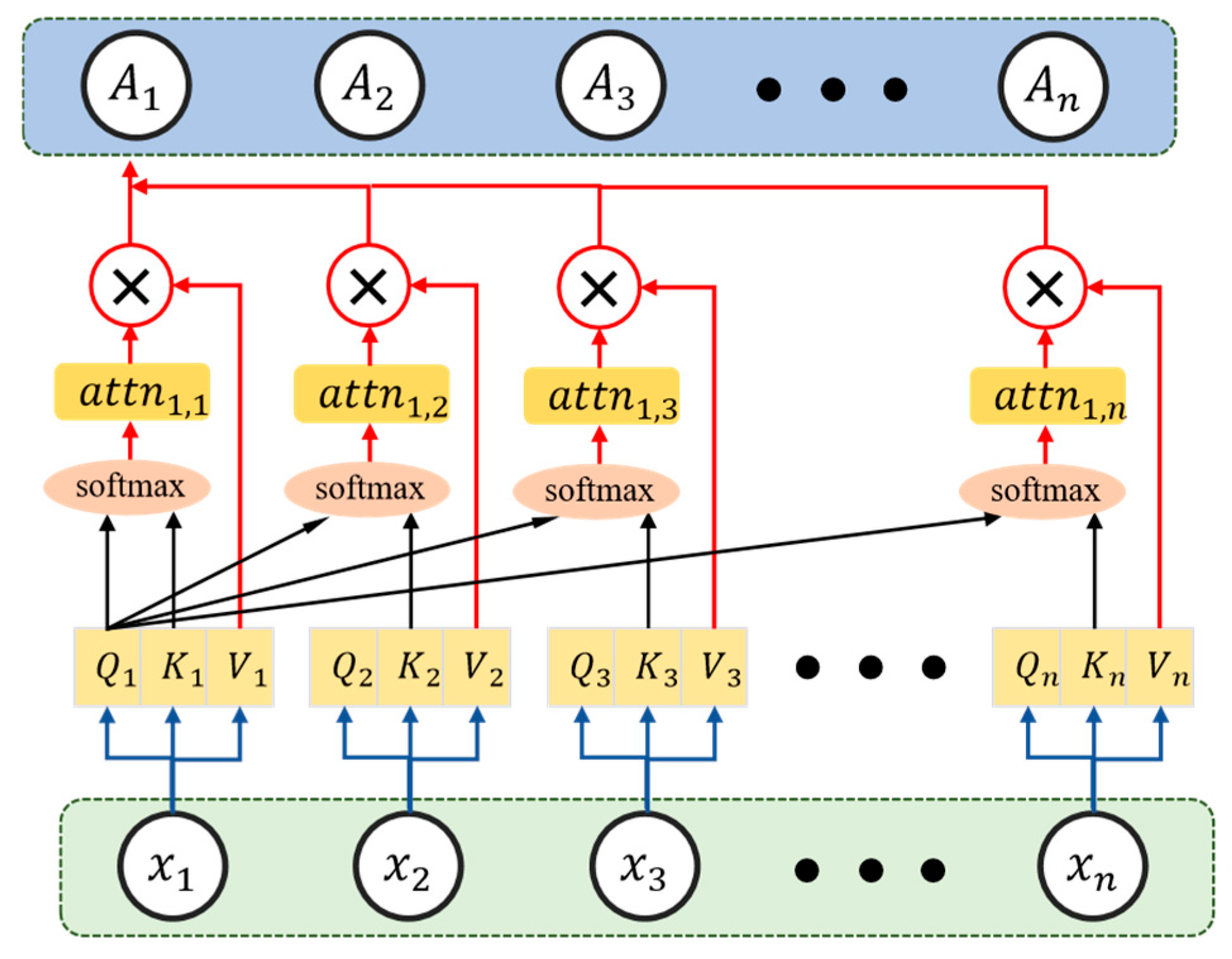
The principle can be summarized as follows: First, attention weights are computed by taking the dot product of the query vector (Q) and the key vector (K). Then, these weights are applied to the value vector (V), yielding a weighted sum of the value vectors across all positions in the sequence. This process produces the output for each time step, as detailed in Equations (6)–(10). The working mechanism of self-attention is illustrated in Figure 3.

$$Q_i=W^q\times x_i$$

(6)

$$K_i=W^k\times x_i$$

(7)

$$V_i=W^v\times x_i$$

(8)

$${\mathrm{attn}}_{i,j}=soft\max \left[Q_i\times {\left(K_j\right)}^T/\sqrt{(d_K)}\right],j=1,2,\dots ,n$$

(9)

$${\mathrm{A}}_i={\displaystyle \sum _{j=1}^n\left(att{n}_{i,j}\times V_j\right)},j=1,2,\dots ,n$$

(10)

Here, $x_i$ represents the feature vector at position iii in the input sequence, $W^q$, $W^k$, and $W^v$ are the weight matrices used to generate Q, K, and V, respectively, $d_k$ denotes the dimension of the key vector, ${attn}_{i,j}$ is the attention weight of position i with respect to position j, and $A_i$ is the final output at position i.

3.3.2. Long Short-Term Memory Network

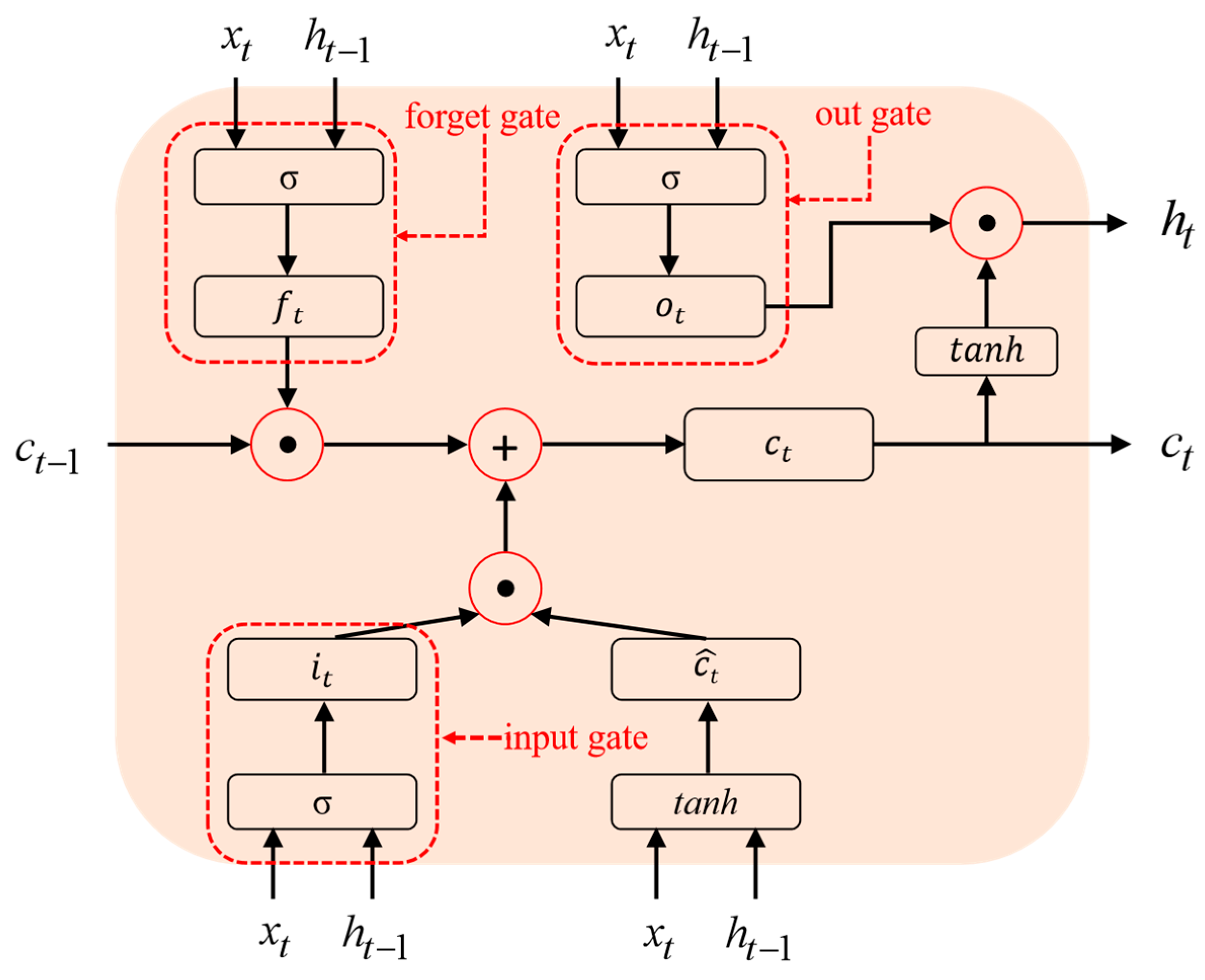
The LSTM utilizes a memory cell that incorporates a gating mechanism to store and update state information from previous time steps. The structure of this gating mechanism is illustrated in Figure 4.

The gated units depicted in the figure encompass the following components: the forget gate $f_t$, which is responsible for discarding irrelevant information from the cell state; the input gate $i_t$, which selectively updates the cell state with new information; and the output gate $o_t$, which governs the output of information [35]. In this context, $x_t$ denotes the input sequence at the current time step, $c_{t-1}$ and $c_t$ represent the memory cell states at the previous and current time steps, respectively, while $h_{t-1}$ and $h_t$ correspond to the hidden states at these two time steps. Additionally, ${\tilde{c}}_t$ signifies the candidate memory cell state at the current time step, with $\sigma$ and tanh serving as the activation functions. The computational process of the memory cell is detailed in Equations (11)–(16).

$$f_t=\sigma \left(W_f\left[h_{t-1},x_t\right]+b_f\right)$$

(11)

$$i_t=\sigma \left(W_i\left[h_{t-1},x_t\right]+b_i\right)$$

(12)

$$o_t=\sigma \left(W_o\left[h_{t-1},x_t\right]+b_o\right)$$

(13)

$${\tilde{c}}_t=\tanh \left(W_c\left[h_{t-1},x_t\right]+b_c\right)$$

(14)

$$c_t=f_t\odot c_{t-1}+i_t\odot {\tilde{c}}_t$$

(15)

$$h_t=o_t\odot \tanh \left(c_t\right)$$

(16)

The terms $W_f$, $W_i$, $W_o$, $W_c$ and $W_c$ represent the weight matrices for different gates and the candidate cell state; $b_f$, $b_i$, $b_o$ and $b_c$ correspond to the respective bias terms; $⨀$ denotes element-wise multiplication.

3.3.3. SA-LSTM Model

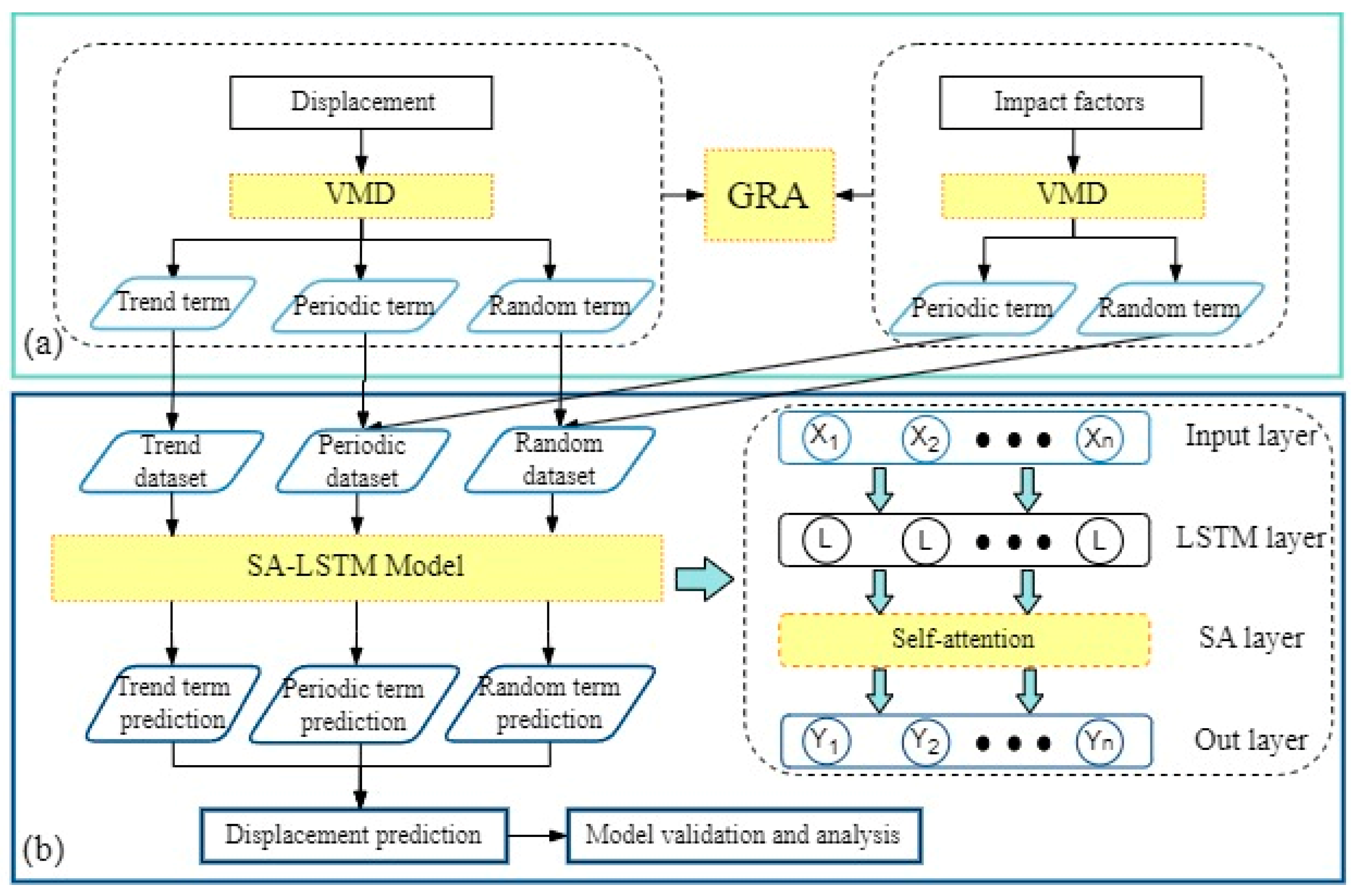
The SA-LSTM prediction model developed in this paper consists of an input layer, an LSTM layer, a self-attention (SA) layer, and a fully connected layer. The basic architecture is illustrated in Figure 5.

The analysis steps are as follows:

• Process the sequential data by the LSTM layer, capturing dependencies between time steps and generating a sequence of hidden states.
• Introduce a self-attention mechanism to further refine the hidden state sequence produced by the LSTM layer,
• Obtain the final prediction result by the fully connected layer (FC layer).

3.4. VMD-SA-LSTM Model

Based on the displacement-time-series theory, VMD theory, and GRA, and incorporating the SA mechanism into the LSTM machine learning algorithm, a dynamic deformation prediction model for the ZVTE landslide has been established. The training process is outlined as follows (Figure 6):

(1)

Extraction of monitoring data

Displacement, rainfall, and other relevant data from the study area were collected. Time periods with significant variation were identified as study intervals, and the types of influencing factors were determined.

(2)

Temporal decomposition

The displacement data and influencing factor data for the target period were decomposed using VMD, followed by a GRA. Suitable displacement and influencing factor components were then selected as input sequences for the model.

(3)

Dataset integration

The displacement trend components were combined with the monitoring time to form the trend dataset. The displacement periodic and random components were, respectively, paired with the corresponding periodic and random components of the influencing factors to create the periodic and random datasets. These datasets were then divided into training and testing sets.

(4)

Model training

The training datasets were separately input into the SA-LSTM model for training, with model parameters adjusted accordingly. The predicted results were then compared and evaluated against the actual data.

(5)

Model validation and analysis

The predicted displacement components were summed to obtain the cumulative landslide displacement predictions, which were then validated and analyzed against the actual cumulative displacement data.

4. Rainfall-Induced Landslide Displacement Prediction

4.1. Landslide Monitoring Data Acquisition and Evaluation Metrics

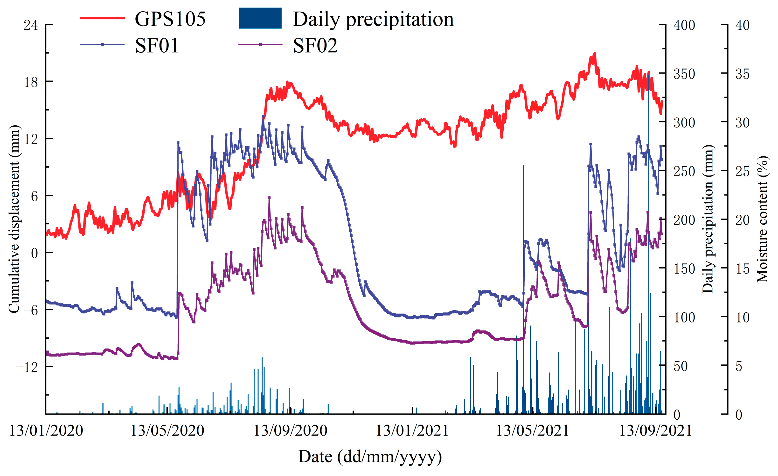
The study collected displacement, rainfall, and soil moisture content data from the GPS105 monitoring point at the ZVTE landslide over a 614-day period, spanning from January 2020 to September 2021. The data from 13 January 2020 to 24 August 2020 were used as the training set, while data from 25 August 2020 to 17 September 2020 were designated as the test set. To evaluate predictive performance, both LSTM and TCN-LSTM models were applied, with the latter combining Temporal Convolutional Networks (TCNs) with LSTM. The inclusion of convolutional layers in the TCN-LSTM model enhances its ability to capture the abrupt deformation features characteristic of landslides [36,37].

To evaluate the predictive performance of each model, the Root Mean Square Error (RMSE), R-squared (R²), and Mean Absolute Percentage Error (MAPE) were selected as metrics. The definitions of these metrics are as follows:

$$\mathrm{MAPE}={\displaystyle \frac{1}{n}}{\displaystyle \sum _{i=1}^n\left|\frac{{\tilde{y}}_i-y_i}{y_i}\right|\times 100\%}$$

(17)

$${\mathrm{R}}^2=1-{\displaystyle \frac{{\displaystyle \sum _{i=1}^n{\left({\tilde{y}}_i-y_i\right)}^2}}{{\displaystyle \sum _{i=1}^n{\left({\overline{y}}_i-y_i\right)}^2}}}$$

(18)

$$\mathrm{RMSE}=\sqrt{{\displaystyle \frac{1}{n}}{\displaystyle \sum _{i=1}^n{\left({\tilde{y}}_i-y_i\right)}^2}}$$

(19)

In these equations, ${\mathrm{y}}_i$ represents the actual observed values, ${\overline{y}}_i$ is the arithmetic mean of the observed values, ${\tilde{y}}_i$ represents the model’s predicted values, and n is the total number of predictions. A smaller RMSE and MAPE, along with an ${\mathrm{R}}^2$ value closer to 1, indicate better model predictive performance.

The study implemented the models using the PyTorch 2.3.0 framework, with the code written in Python 3.9. To facilitate a comparative analysis of model performance, the Adam optimizer was employed during model training to adjust inter-layer weights, with the learning rate set at 0.001. The Mean Squared Error (MSE) was chosen as the loss function, and the LSTM model was configured with 2 layers and 64 hidden units. To prevent overfitting during training, a dropout rate of 0.05 was applied to certain layers.

4.2. Time-Series Decomposition

(1)

Cumulative displacement decomposition

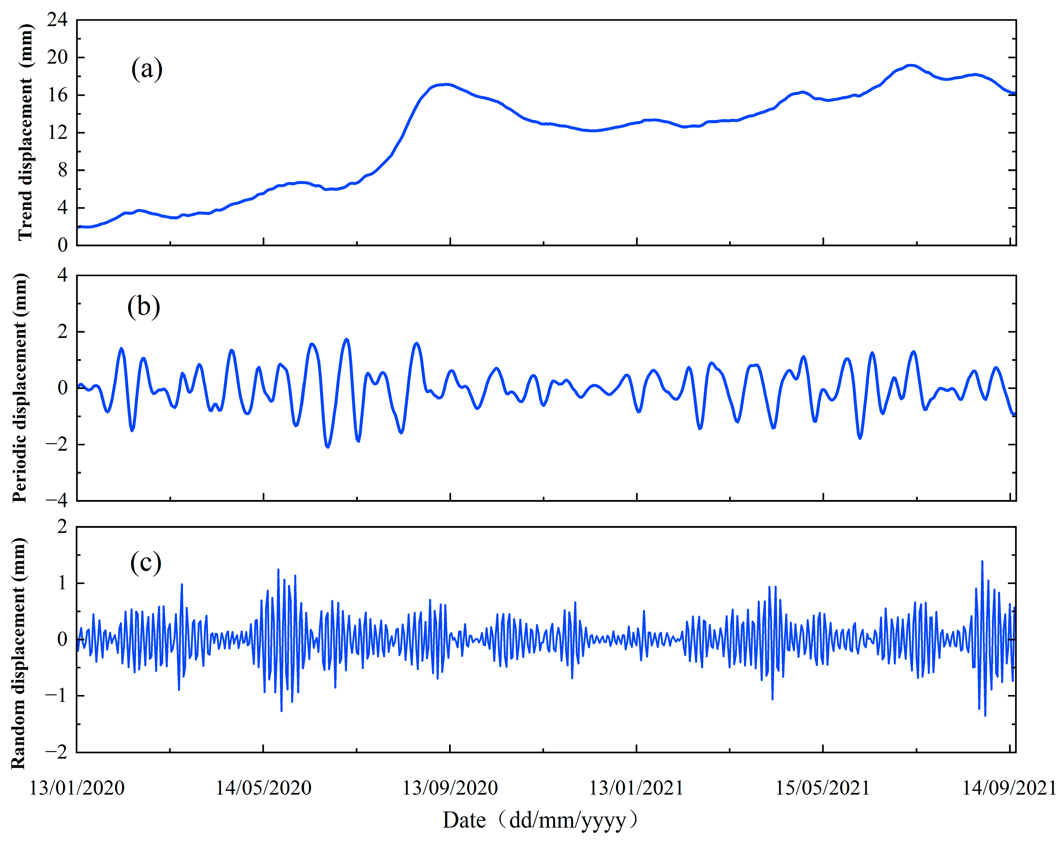
To accurately decompose displacement data and avoid issues of under- or over-decomposition, it is essential to predefine the number of modes. Given the nonlinear dynamic characteristics of landslide displacement, the number of decomposition modes K was set to 3 when applying VMD to the cumulative landslide displacement data. Each mode corresponds to the influence of distinct factors as follows:

-

Trend displacement—the deformation resulting from internal geological conditions.

-

Periodic displacement—the deformation influenced by periodic rainfall.

-

Random displacement—the deformation caused by random external factors, such as non-seasonal rainfall and human activities.

The decomposition results for the cumulative displacement at the GPS105 landslide monitoring point are presented in Figure 7.

(2)

Influencing factor decomposition

Rainfall is a primary factor in inducing shallow landslides, with changes in soil moisture content serving as a direct indicator of the soil’s response to rainfall infiltration. Continuous rainfall increases the soil moisture content on the slope, which softens the soil and disrupts the gravitational balance of the landslide. This process leads to an increase in downslope forces and a reduction in slope stability, resulting in surface displacement and deformation of the landslide body [38,39,40]. Rainwater infiltration into unsaturated soil further raises water content, decreasing matric suction and reducing soil shear strength, which accelerates slope deformation and failure [41]. Therefore, the development of landslides is closely linked to variations in rainfall and soil moisture content. In this study, daily rainfall and soil moisture content are identified as key influencing factors of deformation. When conducting VMD on daily rainfall and water content data, the number of modes was set to K = 2, as the selected influencing factors show no significant trends and are primarily characterized by periodic variations. The decomposed low-frequency component represents the periodic variations of the influencing factors, while the high-frequency component reflects random fluctuations [42,43,44].

4.3. Displacement Component Correlation Analysis

To validate the appropriateness of the selected influencing factors, a correlation analysis between the cumulative landslide displacement components and the influencing factors was conducted [17,45,46]. GRA theory was applied to compare the correlations between different sequences, with the distinguishing coefficient set to ξ = 0.5. A correlation value closer to 1 indicates a higher degree of association between the input variables. The correlation results for each component are presented in

Table 1. Analysis of the correlation between displacement components and influencing factors.

Displacement Component	Influencing Factors
	Daily Rainfall	Moisture Content W1	Moisture Content W2
Trend term	0.5334	0.6281	0.6403
Periodic term	0.5650	0.5888	0.6188
Random term	0.5641	0.5821	0.6124
Cumulative displacement	0.7017	0.6631	0.6778

Note: W₁, W₂ correspond to measurement points SF01 and SF02, respectively.

.

The correlation analysis results reveal that the correlation values between all influencing factors and displacement components exceed 0.5, indicating a strong relationship between the selected factors and displacement components. Specifically, the high correlation values between daily rainfall and both the periodic and random displacement components suggest that seasonal periodic rainfall and non-seasonal random rainfall exert varying degrees of influence on these components. Furthermore, the correlation values between soil moisture content at measurement points $W_1$ and $W_2$ and the displacement components are generally higher than those between daily rainfall and the displacement components. This suggests that changes in soil moisture content have a more direct impact on landslide displacement than rainfall. The correlation between soil moisture content at different measurement points and the periodic and random components of cumulative displacement varies, with measurement point $W_2$ showing higher correlation values with each displacement component. This implies that localized soil moisture conditions have differing effects on the changes in the periodic and random components of displacement.

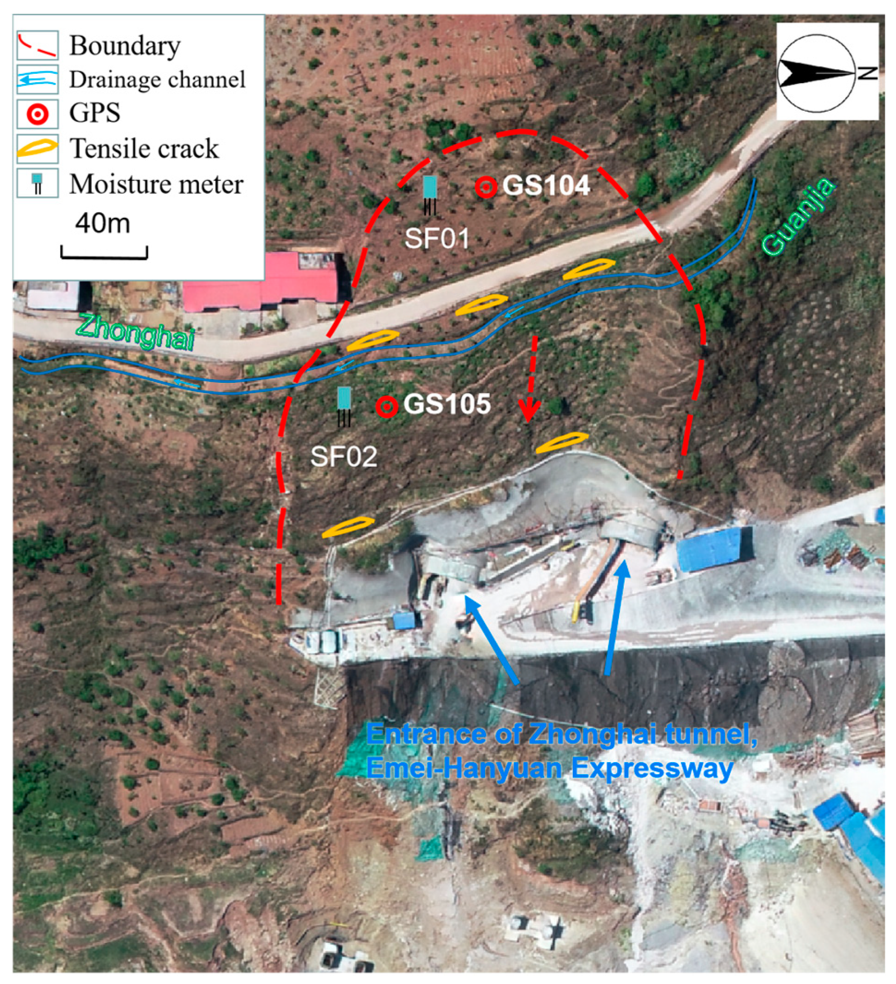
Given that the landslide is of the traction type, excavation at the slope toe for tunnel construction initiated slope body deformation, which was further aggravated by construction vibrations and rainfall. Additionally, leakage from the drainage channel facilitated the formation of the slip surface and accelerated surface instability and downslope movement. Consequently, changes at the landslide’s front edge became more pronounced, and the correlation between water content and displacement was stronger in regions close to the front edge.

4.4. Displacement Prediction

(1)

Trend component displacement prediction

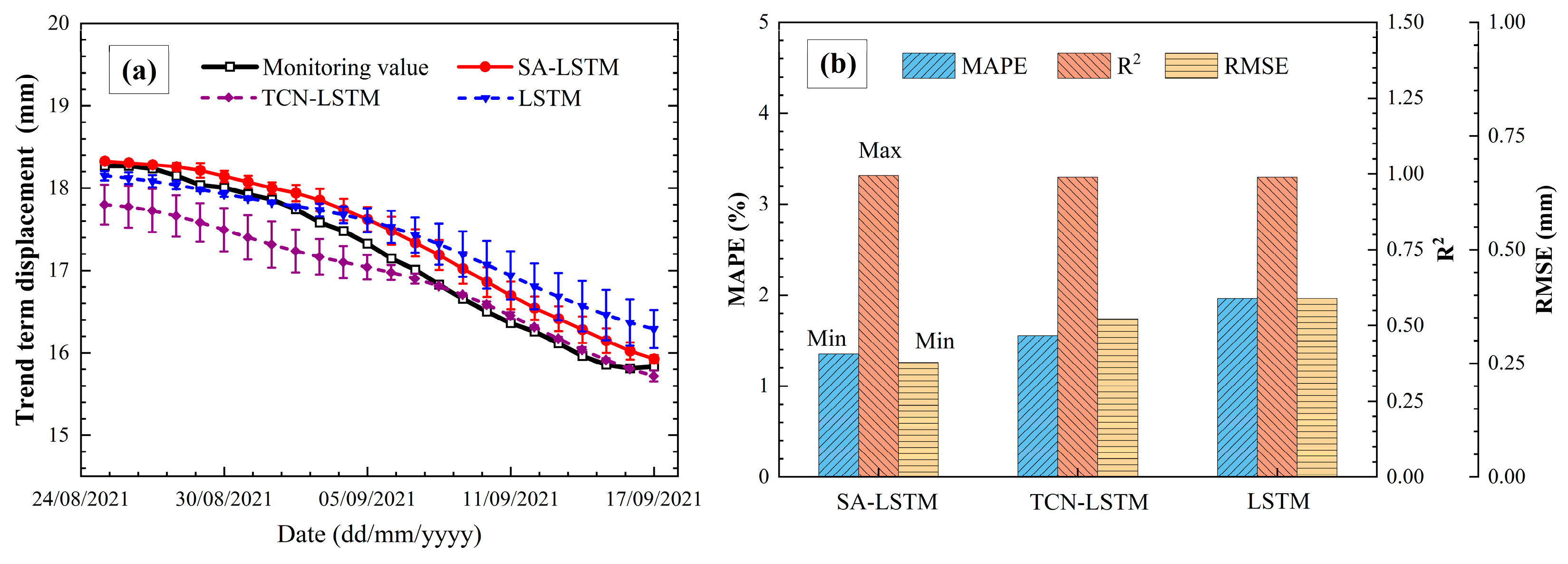
The trend component of displacement, primarily influenced by internal geological factors, was predicted using the SA-LSTM model. The performance of this model was then compared to traditional LSTM and TCN-LSTM models, with the results presented in Figure 8. As illustrated in Figure 8a, t the displacement changes in the trend component remain stable, and all models generate predictions that closely match the observed values. Although the LSTM model shows accurate predictions in the initial phase, it significantly deviates in the later stages. Furthermore, as shown in Figure 8b, incorporating the self-attention mechanism into the LSTM model enhances its ability to capture long-term dependencies in the landslide displacement sequence, outperforming the traditional LSTM and yielding better predictions than the TCN-LSTM model.

(2)

Periodic component displacement prediction

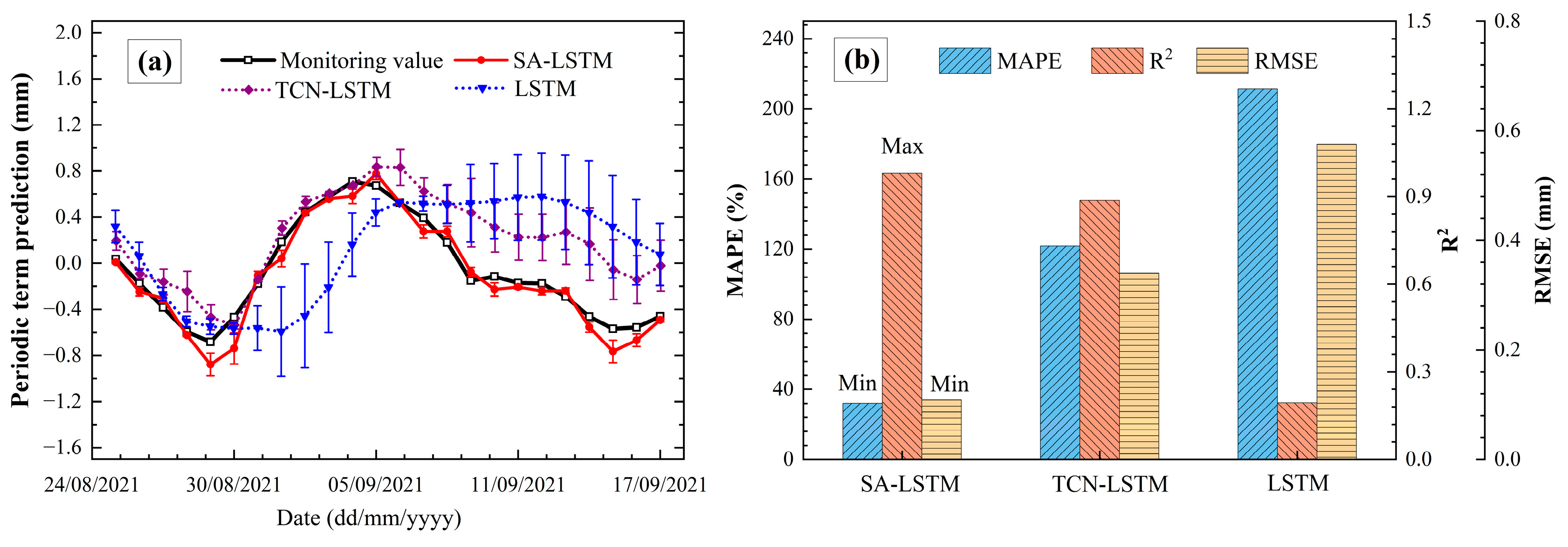
The periodic component of displacement is closely linked to cyclical rainfall and the resulting changes in soil moisture content due to infiltration. The positive feedback loop between these two factors plays a crucial role in driving landslide deformation. To predict the periodic displacement, the dataset for the periodic component was input into various models, with the predictive performance of each model presented in Figure 9.

As illustrated in Figure 9a, the periodic component exhibits significant fluctuations, leading to larger prediction errors with the traditional LSTM algorithm. This suggests that a standard LSTM model struggles to effectively learn when confronted with complex input features. The TCN-LSTM, which processes data through a series of convolutional layers, effectively extracts local features due to its multi-layer convolutional structure. However, it has limitations in capturing the global dependencies between periodic displacement and the periodic components of influencing factors. In contrast, the SA-LSTM model, which incorporates a SA mechanism, assigns weights to all input features and identifies key time points within the sequence. This enables the SA-LSTM to better learn the intricate relationships between periodic changes in rainfall and moisture content and the periodic component of cumulative displacement.

As shown in Figure 9b, the SA-LSTM model achieves better predictive performance, with significantly improved accuracy compared to the LSTM. The SA-LSTM’s prediction results exhibit lower MAPE and RMSE values than both the TCN-LSTM and LSTM models, indicating its superior ability to learn complex deformation mechanisms.

(3)

Random component displacement prediction

The random component of displacement is primarily influenced by external random factors such as non-seasonal rainfall and drainage channel. This random component dataset was input into various models, and their predictive performance was evaluated, as shown in Figure 10.

As shown in Figure 10a, the random component exhibits high-frequency fluctuations, resulting in poor predictive performance by the LSTM and TCN-LSTM models. These models have limited capacity to learn the complex multivariable patterns inherent in the data. In contrast, the SA-LSTM model demonstrates superior performance in capturing these intricate patterns. Figure 10b further illustrates that the SA-LSTM model achieves the lowest RMSE and MAPE values, indicating the highest accuracy among the models.

(4)

Cumulative component displacement prediction

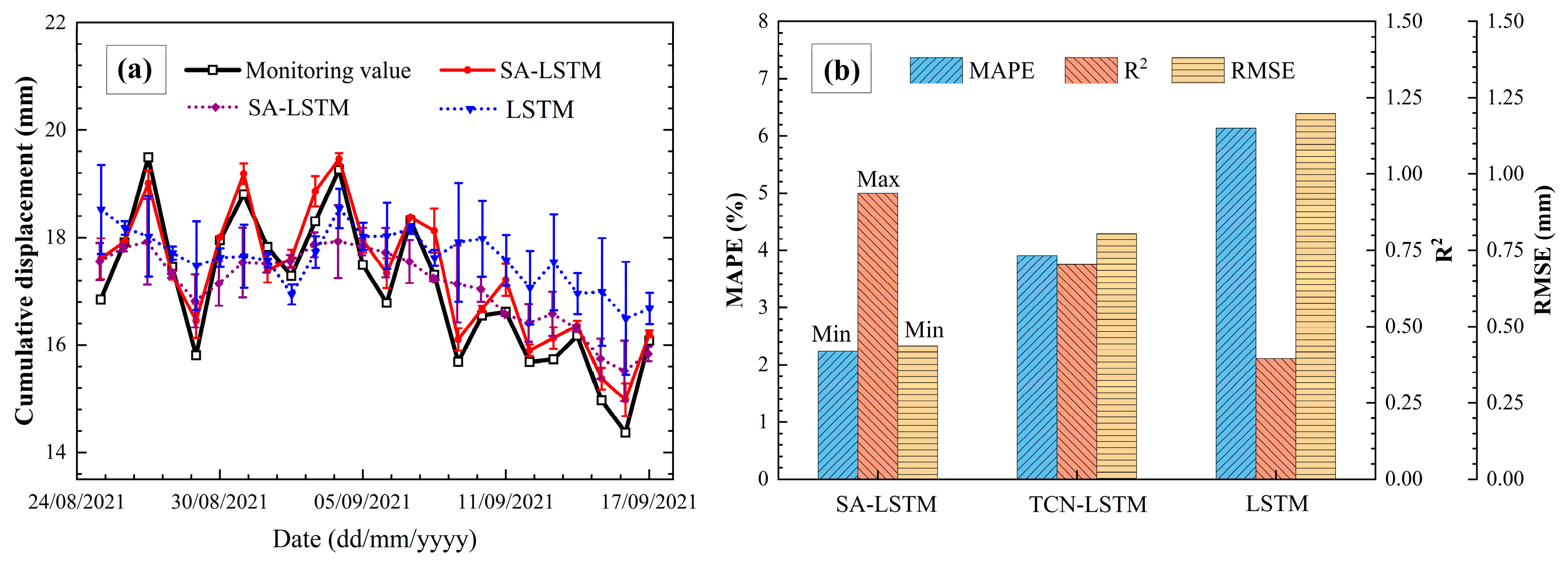
The cumulative displacement of the landslide is calculated by summing the predicted displacement components, with the results for each model illustrated in Figure 11. When external factors introduce complex variations in the landslide deformation curve, the traditional LSTM model faces difficulties in effectively capturing the input features across the entire time series. In contrast, LSTM models enhanced with TCN or SA mechanisms improve the extraction of input features and increase attention to key factors influencing displacement, such as rainfall and soil moisture content. This enhancement leads to varying degrees of improvement in the accuracy of displacement trend predictions. Specifically, the SA-LSTM model, leveraging its SA mechanism, excels at capturing long-term dependencies and global information from historical displacements, resulting in superior predictive performance.

4.5. Discussion

(1)

An evaluation of the displacement prediction results

Table 2. Prediction accuracy and error of landslide displacement models.

Displacement Component	RMSE (mm)			R2			MAPE (%)
	SA-LSTM	TCN-LSTM	LSTM	SA-LSTM	TCN-LSTM	LSTM	SA-LSTM	TCN-LSTM	LSTM
Trend term	0.2520	0.3475	0.3931	0.9944	0.9890	0.9891	1.3541	1.5540	1.9623
Periodic term	0.1090	0.3405	0.5757	0.9799	0.8866	0.1946	32.1264	121.8948	211.4241
Random term	0.3190	0.6596	0.7300	0.8664	0.6903	0.2300	58.9588	84.8986	112.2769
Cumulative displacement	0.4372	0.8048	1.1982	0.9377	0.7035	0.3950	2.2320	3.9094	6.1306

presents the predictive performance metrics for each algorithm model concerning the displacement components. The SA-LSTM model consistently outperforms the others, achieving the lowest RMSE and MAPE values and the highest R², indicating superior accuracy across all displacement components. Specifically, for the final cumulative displacement prediction, the SA-LSTM model records RMSE and MAPE values of 0.4372 and 2.2320, respectively. These values reflect reductions of 45.676% and 42.907% compared to the TCN-LSTM model, and 63.512% and 63.592% compared to the traditional LSTM model. This significant improvement in accuracy highlights the SA-LSTM model’s superior predictive performance.

The traditional LSTM model, with its unique internal gating mechanism, memorizes and adaptively extracts historical information from input landslide features. However, due to the inherent randomness in its gating mechanism during training, LSTM models face challenges in predicting rapidly changing displacement components, resulting in substantial prediction errors. This limitation reduces the model’s ability to capture short-term, sharp fluctuations. In contrast, both TCN-LSTM and SA-LSTM models exhibit superior performance in feature extraction from complex time-series data. While TCN is adept at capturing local variations, SA-LSTM excels in managing long-term dependencies. The self-attention mechanism in SA-LSTM enhances global learning and assigns weights to all historical state features extracted by the LSTM, with particular emphasis on the time steps associated with external factors. This approach significantly improves the model’s ability to detect changes in soil conditions and mechanical properties caused by increased rainfall and moisture content. By adaptively adjusting the weights of critical influencing factors, SA-LSTM enhances the accuracy of landslide displacement predictions.

(2)

Model applicability

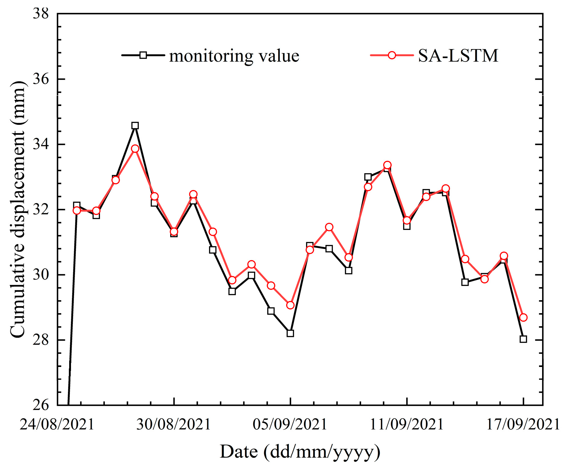
The proposed SA-LSTM model was applied to predict the displacement at an additional monitoring point, GPS104, located at the tunnel entrance of the ZVET landslide. Since GPS104 is situated on the same landslide as the previous measurement points, the same influencing factors were used for this analysis. The displacement components of GPS104, together with the influencing factors, were combined to create datasets for the trend, periodic, and random components, which were then utilized for displacement prediction. The resulting cumulative displacement predictions are shown in Figure 12 and

Table 3. Prediction accuracy and error of cumulative displacement at GPS104.

Measurement Point	RMSE (mm)	R2	MAPE (%)
GPS104	0.4232	0.9727	1.0387

. The proposed model achieved high accuracy in predicting displacement at monitoring point 104, with RMSE of 0.4232 and MAPE of 1.0387. These results demonstrate the SA-LSTM model’s effectiveness in learning and predicting deformation trends across multiple monitoring points within the same landslide, confirming its generalization capability and robustness in multi-point prediction.

5. Conclusions

To address the challenge of the insufficient extraction of complex features from long time series in deep learning methods for multivariable landslide displacement prediction, this study develops a deep learning time-series prediction model based on Variational Mode Decomposition (VMD) and Self-Attention LSTM (SA-LSTM). This model enhances the capacity to retain historical information by integrating a self-attention mechanism into the traditional LSTM framework, effectively capturing the nonlinear characteristics of landslide changes and thereby achieving short-term dynamic predictions of rainfall-induced shallow landslides at the entrance of the Zhonghai Village tunnel. The key findings of this study are as follows:

(1)

The model utilizes Variational Mode Decomposition (VMD) to decompose the cumulative landslide displacement series, effectively addressing the over- and under-decomposition issues often observed in traditional time-series decomposition techniques such as moving average, wavelet analysis, and Empirical Mode Decomposition (EMD). In addition, grey relational analysis (GRA) is employed to evaluate the correlation between the decomposed displacement components and external triggering factors, ensuring the validity of the selected variables. This method not only more accurately captures the influence of external factors on landslide deformation but also enhances the model’s physical interpretability.

(2)

The model utilized soil moisture content and rainfall as influencing factors in a multivariate time-series prediction of displacement. The results demonstrate that incorporating a self-attention mechanism into the SA-LSTM model effectively captures changes in abrupt multivariate data, significantly enhancing LSTM’s predictive performance for both displacement periodic and random components.

(3)

Using the Zhonghai Village tunnel entrance (ZVTE) landslide as a case study, this research employs the SA-LSTM model to predict displacement time series at the GPS105 and GPS104 measurement points. The results indicate strong predictive performance, with RMSE values of 0.4372 and 0.4232 for cumulative displacement, and MAPE values of 2.232 and 1.0387, respectively. These outcomes emphasize the model’s robust generalization ability and prediction stability across multiple measurement points, demonstrating its substantial potential for broader application in time-series analysis and prediction of non-reservoir-type landslides.

While the SA-LSTM model demonstrates excellent predictive accuracy, its reliance on extensive matrix multiplication within the self-attention mechanism significantly increases computational complexity as the input sequence length and feature dimensionality expand. To address this issue and improve training efficiency, future research will explore the use of local attention mechanisms to mitigate computational demands. Moreover, although the model has exhibited strong generalization and predictive stability within a single landslide area, its performance across diverse landslide types remains to be thoroughly validated. Future work will aim to apply the model in various scenarios, such as soil- and earthquake-induced landslides, while flexibly adjusting the model structure to suit different geological conditions and data characteristics. Through these ongoing efforts, the model’s effectiveness in landslide prediction is expected to improve, providing more precise and efficient technical support for early warning systems and disaster prevention in the context of geological hazards.