Article

Predictions of Peak Discharge of Dam Failures Based on the Combined GA and BP Neural Networks

1
College of Hydraulic & Environmental Engineering, China Three Gorges University, Yichang 443000, China
2
China Renewable Energy Engineering Institute, Beijing 100120, China
3
College of Electronic Engineering, Chengdu University of Information Technology, Chengdu 610225, China
4
CMA, Key Laboratory of Atmospheric Sounding, Chengdu University of Information Technology, Chengdu 610225, China
5
School of Mechanical Engineering, Sichuan University of Science & Engineering, Yibin 617000, China
*
Authors to whom correspondence should be addressed.
Water 2024, 16(20), 2946; https://doi.org/10.3390/w16202946
Submission received: 24 September 2024 / Revised: 12 October 2024 / Accepted: 14 October 2024 / Published: 16 October 2024
(This article belongs to the Special Issue Water Engineering Safety and Management)

Abstract

:
In this paper, the Artificial Neural Network (ANN) was utilized to predict the peak discharge of dam failures, which was based on the combined Genetic Algorithm (GA) and Back Propagation (BP) neural network. The dataset comprises 40 samples from self-conducted experiments and available literature. To compare the efficiency of the suggested approach, three evaluation metrics, including the coefficient of determination (R2), the root mean square error (RMSE) and the mean absolute error (MAE), were analyzed for both the BP neural network and the GA-BP neural network. The findings suggest that (1) The prediction accuracy of the GA-BP was better than that of the BP; and (2) Compared to BP, GA-BP demonstrated a 9.07% average improvement in R2, a 57.36% average reduction in MAE, and a 57.53% average reduction in RMSE. In addition, the results of GA-BP and semi-empirical formulas were compared and the effect of three parameters on the peak discharge was analyzed. The results showed that the GA-BP model could effectively predict the peak discharge of dam failures.

1. Introduction

Landslide dams are natural earth and rock dams that can eventually evolve into dammed lakes. As a result, most dammed lakes experience uncontrolled overtopping, which can even lead to dam failures [1]. Dam-break flows pose significant risks to the lives and properties of downstream residents. Due to the complex nature of dam-failure processes, accurately predicting the peak discharge in advance remains challenging [2]. Even calculating/measuring the timely discharge at the dam site is extremely difficult [3,4]. Therefore, developing an effective methodology to accurately predict the peak discharge of dam failures is crucial for disaster forecasting and mitigation downstream [5].
The prediction of peak discharge currently relies on two primary methods: numerical simulation and physical model test [6,7]. Numerical simulation involves modeling rainfall-runoff and river flow processes to estimate peak discharge [8,9]. Wang et al. (2022) developed a model called the Weather Research and Forecasting Model with the Storm Water Management Model (WRF-SWMM) by combining WRF Model with SWMM to forecast urban flood processes, which significantly improved the timeliness of predictions [10]. Takayama et al. (2021) introduced a numerical model for progressive failures, which could effectively predict flood hydrographs [11]. Akazawa et al. (2014) developed a numerical model to simulate landslide dam erosion due to overtopping flow [12]. However, these models are computationally inefficient and not applicable for real-time estimations [13,14].
On the other hand, experimental model testing is another popular method for studying dam-break problems, and a series of empirical formulas have been established [15,16,17]. Walder et al. (2015) found that peak discharge increased linearly with dam height in most cases [15]. Al-Riffai (2014) conducted experiments to analyze breach characteristics and erosion of noncohesive embankments [16]. Peak discharge based on large-scale particle image velocimetry (LS-PIV) was proposed by estimating surface velocities and the breach, supporting its reliability in discharge estimation and dam-failure analysis [17]. It should be noted that these empirical formulas are based on individual experimental data and certain assumptions, such as breach width, initial water depth, and water depth in the breach, leading to the absence of a universal formula up to now.
Given these limitations, establishing innovative methods to improve the prediction accuracy of peak discharge is a necessity. Neural networks, recognized for their nonlinear mapping and self-learning capabilities, have been extensively applied in hydrological forecasting. Guo et al. (2021) implemented an urban flood prediction based on the deep convolutional neural network (CNN) [18]. Simon et al. (2019) proposed a model based on ANNs to predict the maximum water level during flash floods [19]. The results suggested that ANNs could aid real-time flood forecasting. BP neural network excelled at handling complex nonlinear relationships and could be trained to predict the water level or sand volume downstream of the flood [20,21,22]. Ye and Kong (2022) developed a BP model for predicting downstream river flood levels [21]. The Decision Group Back Propagation Network (DGBPN) model proposed by Chen et al. (2010) demonstrated strong adaptability and achieved accurate flood hydrograph predictions in the Wu-Shi watershed in Taiwan [22]. However, BP is prone to fail in local optimal solutions [23,24]. In contrast, the Genetic Algorithm (GA) can offer strong global search capabilities, thus effectively addressing this limitation [25,26,27]. Liu et al. (2024) [28] employed a GA-BP neural network to forecast the seepage volume of shale reservoirs, and the relative error was within 6%. Zhang et al. (2023) [29] studied the energy consumption of office buildings in cold regions based on BP and GA-BP, and GA-BP outperformed BP by 38.89% in RMSE. GA was used to optimize the ANFIS model and reliability was improved compared to the ANFIS model [30,31,32]. Thus, integrating GA with other methods is a promising way to enhance the global search ability and prediction accuracy [33].
This paper proposes an ANN method that integrates GA with BP to predict the peak discharge of dam failures. Although GA-BP has been widely used in other fields, its effectiveness in predicting the peak discharge of dam failures has not been reported so far. In this method, the traditional backpropagation process in BP is replaced by GA operations, including selection, crossover, and mutation. Each signal is utilized as input data to construct a GA-BP model. The ultimate peak discharge is obtained by integrating the predicted data from each signal. Additionally, this study compares the performances of the BP and GA-BP models by using various performance metrics. The paper is organized as follows: Section 2 outlines the self-conducted experiments and gives all samples; Section 3 introduces the GA-BP neural network; conclusions are presented in Section 4.

2. Problem Descriptions and Database

Physical modeling experiments were conducted to investigate the dam-failure process, and all tests were taken as the samples in the below ANN-based prediction. Due to the scale effects of the physical model, additional samples were sourced from the literature. These combined data will serve as the total samples. Prior to the ANN-based prediction of the peak discharge, the experimental setup and measured data were exampled and discussed.

2.1. Experimental Setups and Results

2.1.1. Experimental Setups

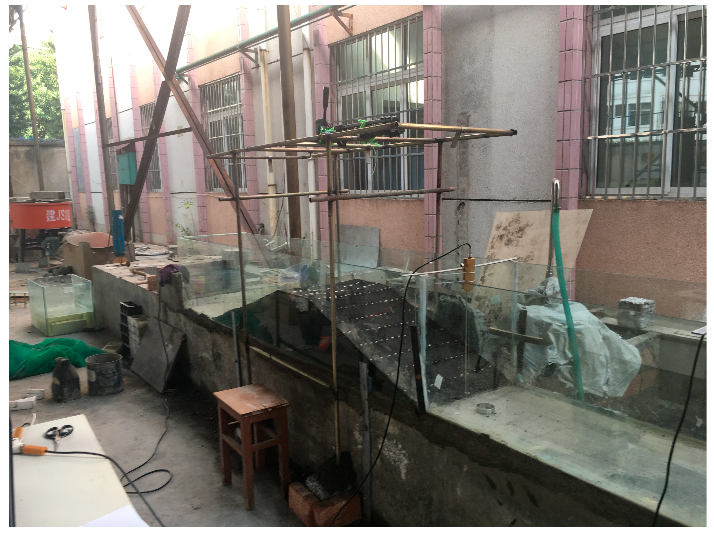
The experimental facilities consisted of an L-shaped glass flume with dimensions of 8.8 m in length, 0.4 m in width, and 0.75 m in height, one wave gauge, and two digital cameras (Chengdu Xinda Shengtong Technology Co., Ltd., Chengdu, China). The flume was divided into two parts: a test section with a length of 7.0 m and a sedimentation tank with a length of 1.8 m, as shown in Figure 1. The wave gauge LG1 was positioned along the centerline of the flume at 2.0 m upstream of the dam. Two digital cameras (Dv1 and Dv2) were placed, respectively, above and on the side of the dam. A right-angle triangular weir was installed in the downstream sedimentation tank. This study considered the effects of dam material, dam slope (upslope and downslope), dam configuration, presence of slotting, and reservoir capacity on dam-failure discharge. To maintain consistency, all materials had the same gradation. The slopes were formed using molds, and during the filling process, the material was compacted every 0.1 m using a wooden tamper. The compacted height was approximately 0.02 m above the design height. Finally, we used a weight of 20.0 kg to statically compress the dam for one hour. The degree of compaction was classified as “high”, “medium”, and “low” by AI-RIffai (2014) [16], with the present dam being categorized as “medium”. The experimental site layout is displayed in Figure 2. All instruments were calibrated and were synchronously activated when the water depth reached a level of 2.0 cm below the dam crest. When the water reached the dam top and the overflow starts, the inflow was simultaneously closed.

2.1.2. Summary of Experimental Tests

We conducted fourteen tests, and their details are presented in Table 1. From this table, the dam height (Hd) varied from 0.15 m to 0.30 m, the storage capacity (Sc) was between 0.282 m3 and 0.564 m3; the median diameter (D50) and porosity (P) were constant, equaling to 2.500 mm and 0.512 mm, respectively. Ld represents the width of the dam in the width direction perpendicular to the water flow. We also studied dams with and without slotting, with additional parameters summarized in Table 1.
Tests 1 to 3 evaluated the repeatability of the experimental model, while tests 4 and onwards gradually altered various parameters to examine their effects on the peak discharge. Test 4 showed that slotting can mitigate the peak discharge. In tests 5 to 7, peak discharge increased as the dam crest and base widths were reduced. Additionally, tests 9 to 12 indicated that an increase in dam height had little effect on the peak discharge. Tests 13 and 14 demonstrated that a reduction in storage capacity for the same dam configuration decreased the peak discharge.
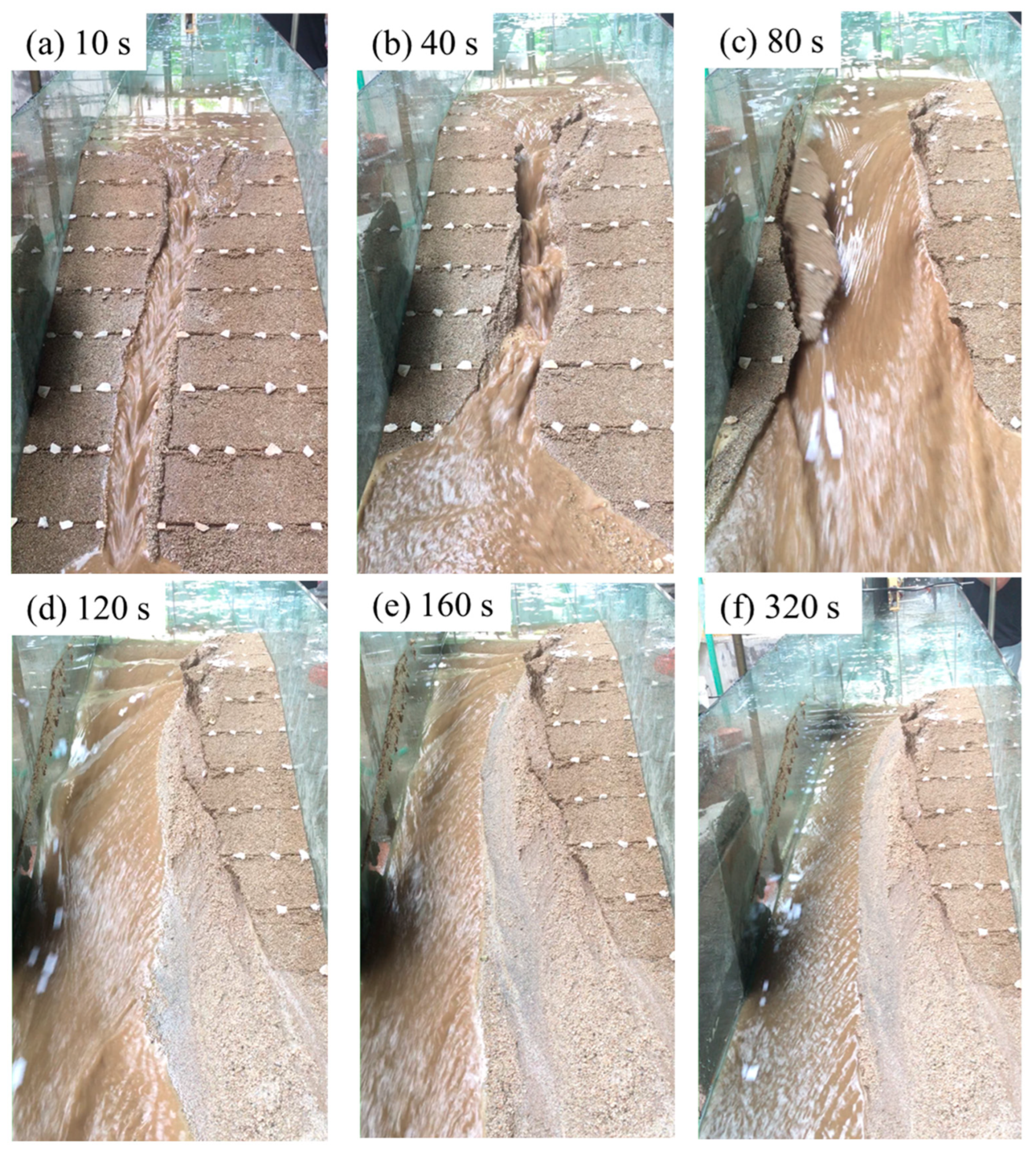
For a demonstration, the experimental snapshots of test 1 at various instants are displayed in Figure 3. An initial breach was formed on the downslope after water flows over the dam crest (see Figure 3a). Then, the flow around the breach moved slowly, and meantime, along with a larger downstream velocity, it moved over that of the transverse (see Figure 3b). As the erosion grew, the flow discharge increased, leading to a quick expansion of the breach with intermittent slope collapses (see Figure 3c). Additionally, because of the absence of the inflow upstream, the dam was not completely eroded. After that, the breach gradually came to a steady state (see Figure 3d–f).

2.2. Summary of Available Data

Table 2 lists some experimental data in literature [15,16,17]. From this table, the dam height ranges from 0.10 m to 1.02 m. The crest width covers a range from 0.011 m to 1.785 m. Three dam widths, namely 1.5 m, 2.0 m and 4 m, are included. It is noted that a higher dam always yields a larger peak discharge [15], while narrower dams lead to a larger peak discharge [16]. The D50 also influences the peak discharge, and a smaller D50 generally but not exactly results in a lower peak discharge. Eventually, a total of 40 samples were obtained from both autonomous experiments and literature, including 9 parameters.

3. Details of the Neural Network

3.1. GA Network

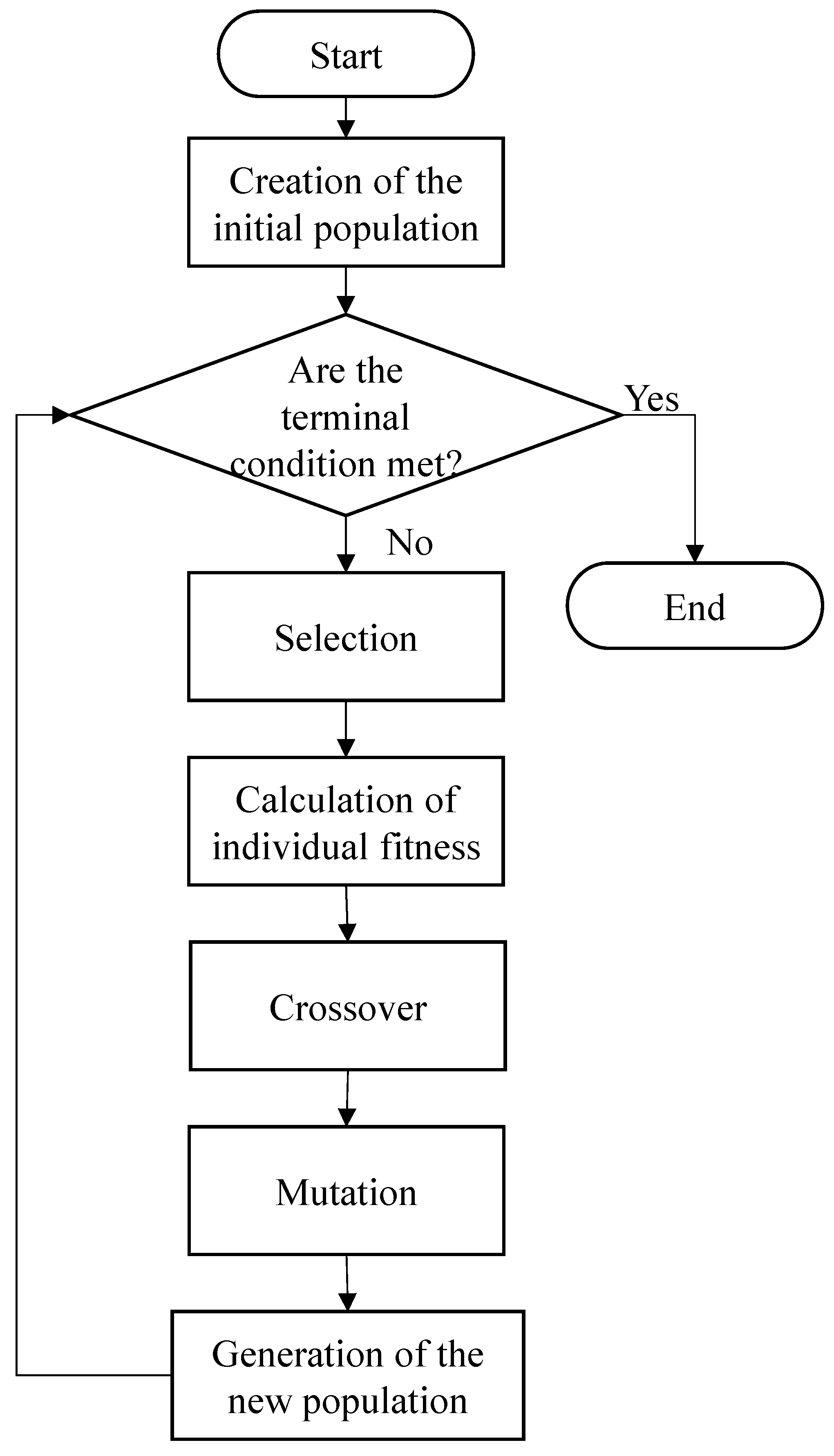
The GA network is an evolutionary algorithm designed to seek globally optimal solutions by using selection, crossover, and mutation to avoid getting stuck in locally optimal solutions. Each chromosome represents a feasible solution to the problem. The fitness function is used to determine if an individual within the current population of chromosomes meets specific properties. If it satisfies the requirements and is deemed the optimal solution, the process concludes. Otherwise, the current population of chromosomes will evolve into a new population through crossover and mutation operations, continuing until individuals that meet specific termination criteria appear in some generation of the population. The flow chart of the GA is illustrated in Figure 4. It iteratively searches for the globally optimal solution until the specified condition is met. However, GA depends on the stochastic search and an evolutionary process, which have the deficiencies of convergence inefficiency and uncertainty of fitness.

3.2. BP Model

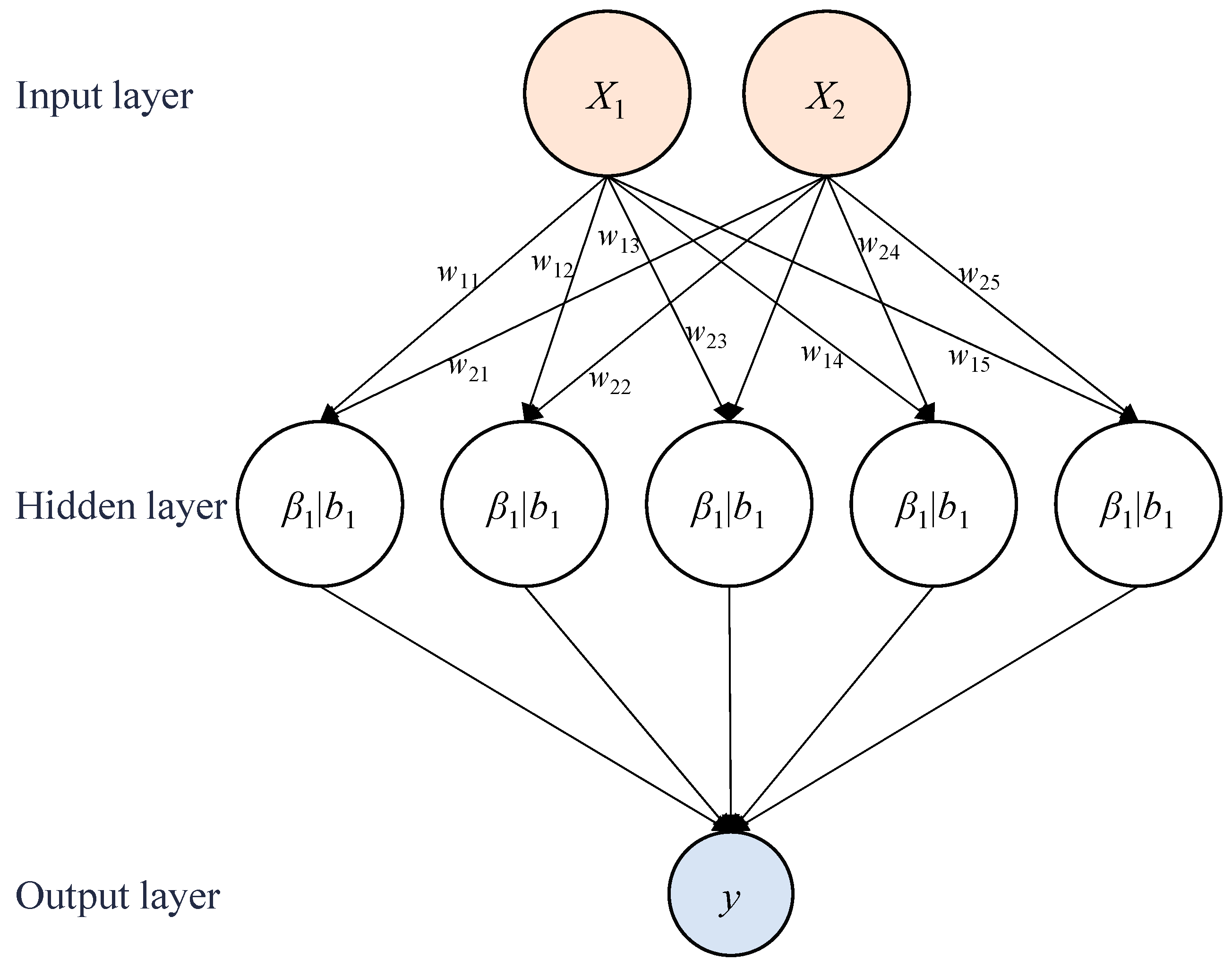
BP is a multilayer feedforward network trained by the backpropagation algorithm. The core of BP is to transmit data through forward propagation and reduce errors through backward propagation. The network consists of multiple neurons, and each neuron processes the input by using an activation function, which will then be passed on to the next neuron. The structure of BP is composed of input, hidden, and output layers (see Figure 5). The data in the input layer are transmitted to the hidden layer with the associated weights (Wij), and the output layer gives the final solution.
1. Xi: input data; 2. Wij: weight; 3. βi: bias.
The logsig formula is chosen as the activation function [34], as follows:
f ( x ) = 1 1 + e x
Data in the hidden layer are expressed as the below formula:
l o g s i g ( X i W i j + X i + 1 W i j + 1 + β i )
The result is determined by Equation (3), as follows:
y = m = 0 m < 5 l o g s i g ( W m i = 0 i < 2 j = 0 j < 5 W i j X i + β j + β y )
To adjust weights and calculate the mean squared error (MSE) function, the gradient descent method is used in BP [34], which can be described in Equation (4):
E ( W , b ) = 1 m i = 1 m 1 k j = 1 k ( y i j ^ y i j ) 2
where m is the number of training samples, k is the number of outputs, y i j ^ is the predicted value of the k-th output of the i-th sample, and yij is the real value of the k-th output of the i-th sample. The output reaches the appropriate value when the expectation is met. The iterative process of weight is shown in Figure 6.

3.3. Developed the GA-BP Neural Network

The BP relies on gradient information, and it may struggle to find the globally optimal solution when the initial weight is not appropriate, or the training data are noisy. In contrast, the GA excels at global search. Combining GA and BP can enhance the performance of the backpropagation process by integrating their advantages in optimizing the initial weight and reducing error. The flow chart of GA-BP is illustrated in Figure 7. Unlike the original BP, the present backpropagation process is fulfilled by three steps: selection, crossover and mutation (see the red box in Figure 7). The optimization process involves three key aspects, as follows:
  • A set of combinations of weight and bias is considered as an individual.
  • The error between the output and the real value is taken as the fitness function of GA.
  • Through finite iterations, the individual with the highest fitness is considered the optimal value of the network.
In this study, the number of input layers, hidden layers, and output layers of GA-BP neural network were constant and equal to 1. The number of input units was equivalent to the number of parameters. The number of units in the hidden layer was set as 5. Through multiple experimentations, the results showed that these parameters yield favorable performance on both the training and test sets. Furthermore, increasing the number of hidden layers or units did not significantly enhance the performance of network, which could instead result in an increase in the training time.

3.4. Performance Evaluation of the Neural Network

To evaluate the performance of BP and GA-BP, three metrics are commonly used, including R2, RMSE and MAE [35], which are calculated by Equations ((5)–(7)), as follows:
R 2 = ( T S S R S S ) / T S S
RMSE = i = 1 n ( y i y i ^ ) 2 / n
MAE = i = 1 n y i y i ^ / n
where TSS is the total sum of squares, equaling to T S S = i = 1 n ( y i y ¯ ) 2 ; RSS is the residual sum of squares, defined as R S S = i = 1 n ( y i y i ^ ) 2 . yi represents the i-th real value, y ¯ represents the mean of real values, y i ^ represents the i-th predicted value, and n denotes the number of samples.
Cross-validation is a technique employed to assess the performance of two networks on unseen data and to prevent overfitting. In this case, we utilized a five-fold cross-validation approach to partition and assess the dataset. The dataset samples were randomly divided into training and test sets in an 80:20 ratio. The training set was used to train the network, and the test set was used to evaluate its performance through five individual runs. The average of the five runs was then taken as the final performance metric.

4. Results and Discussion

The peak discharge of dam failures is predicted by the BP and the GA-BP in this section. The performance evaluation metrics of the two neural networks are analyzed, and the advantages of the improved neural network are discussed. The performance is evaluated based on both accuracy metrics and the incidence of overfitting.

4.1. Prediction of Peak Discharge Based on BP

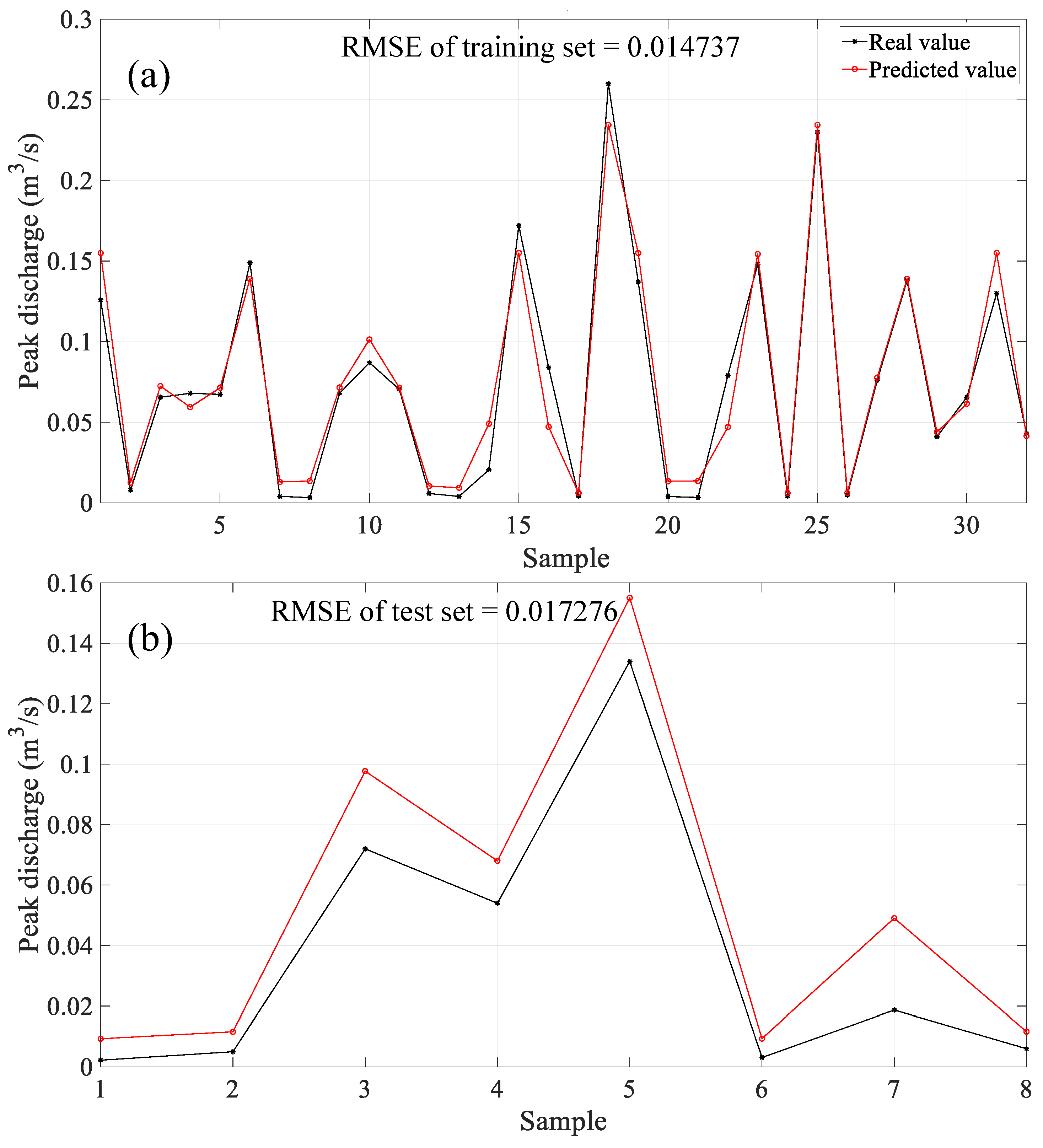
According to the previous statement, the dataset consists of 32 training samples and 8 test samples. Figure 8 gives the comparisons of the predicted peak discharge (red line) with the experimental data (black line) and the RMSE value in one run. The x-axis of the figure represents the predicted sample, while the y-axis represents the peak discharge. From this figure, the RMSEs for the training set and the training set are 0.014737 and 0.017276, respectively, suggesting a strong correlation between the predicted and real values for most samples. However, there are several cases with significant errors. For example, for sample 7 corresponding to case 22 in Table 2, the predicted value is more than twice the real value, potentially due to the weak adaptability of BP to unseen data [23]. The cases with large peak discharges (e.g., case 9, case 10, case 13 in Table 2) pose greater destructive power and are therefore of greater concern. The relative errors of BP prediction for these cases range from 15.60% to 35.07%, within an acceptable range.
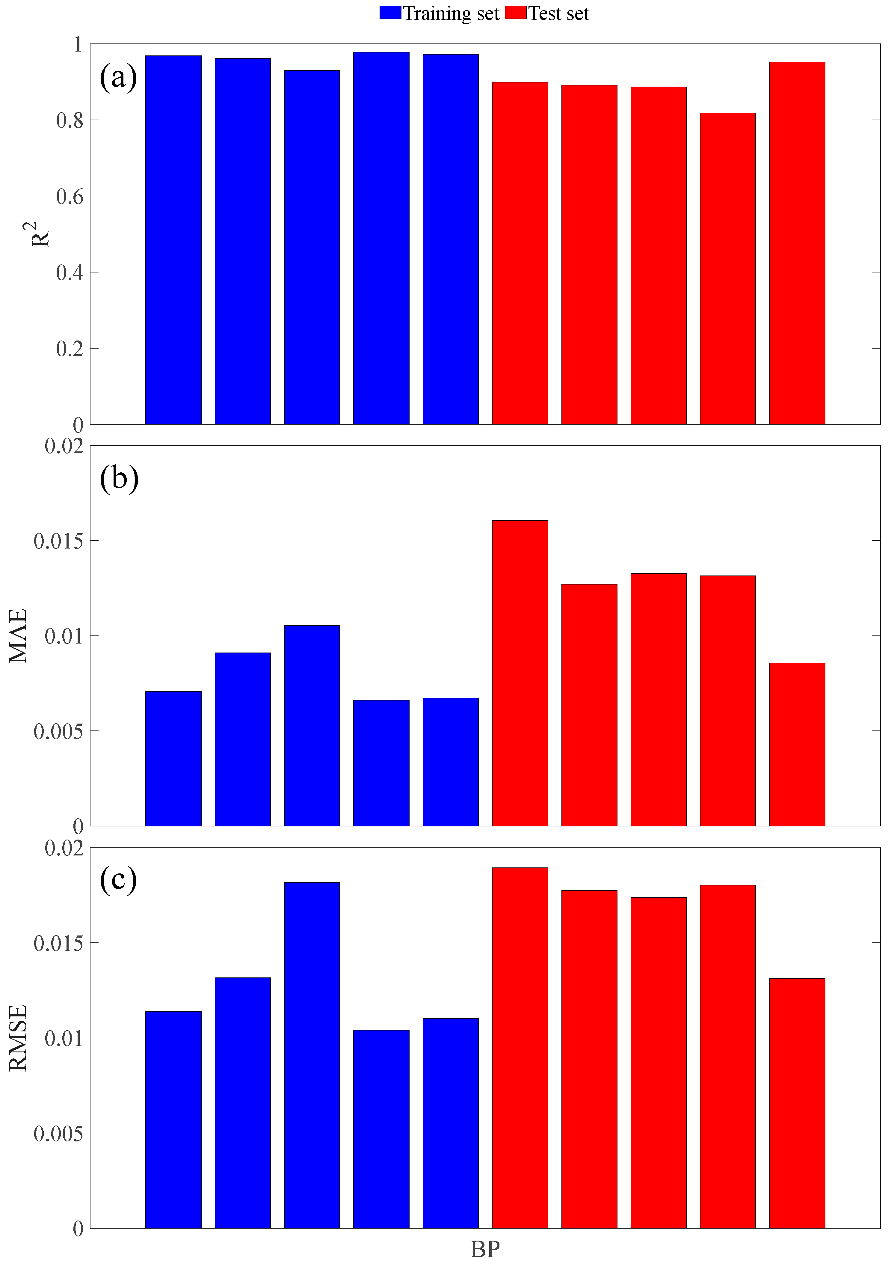
Figure 9 presents the performance evaluation metrics for BP by using the five-fold cross-validation. The larger R2 of the training set indicates that BP can effectively reproduce the training data. However, the R2 of the test set is relatively low, particularly in the fourth run, which is significantly lower than four other runs (see Figure 9a). This suggests that overfitting may have occurred during the training process. In addition, the MAE of the training set is lower than that of the test set, especially in the first run (see Figure 9b), indicating poor performance of the network on unseen data. Although the RMSE slightly increases in the first run, the overall performance of BP for unseen data is considered acceptable.

4.2. Prediction of Peak Discharge Based on GA-BP

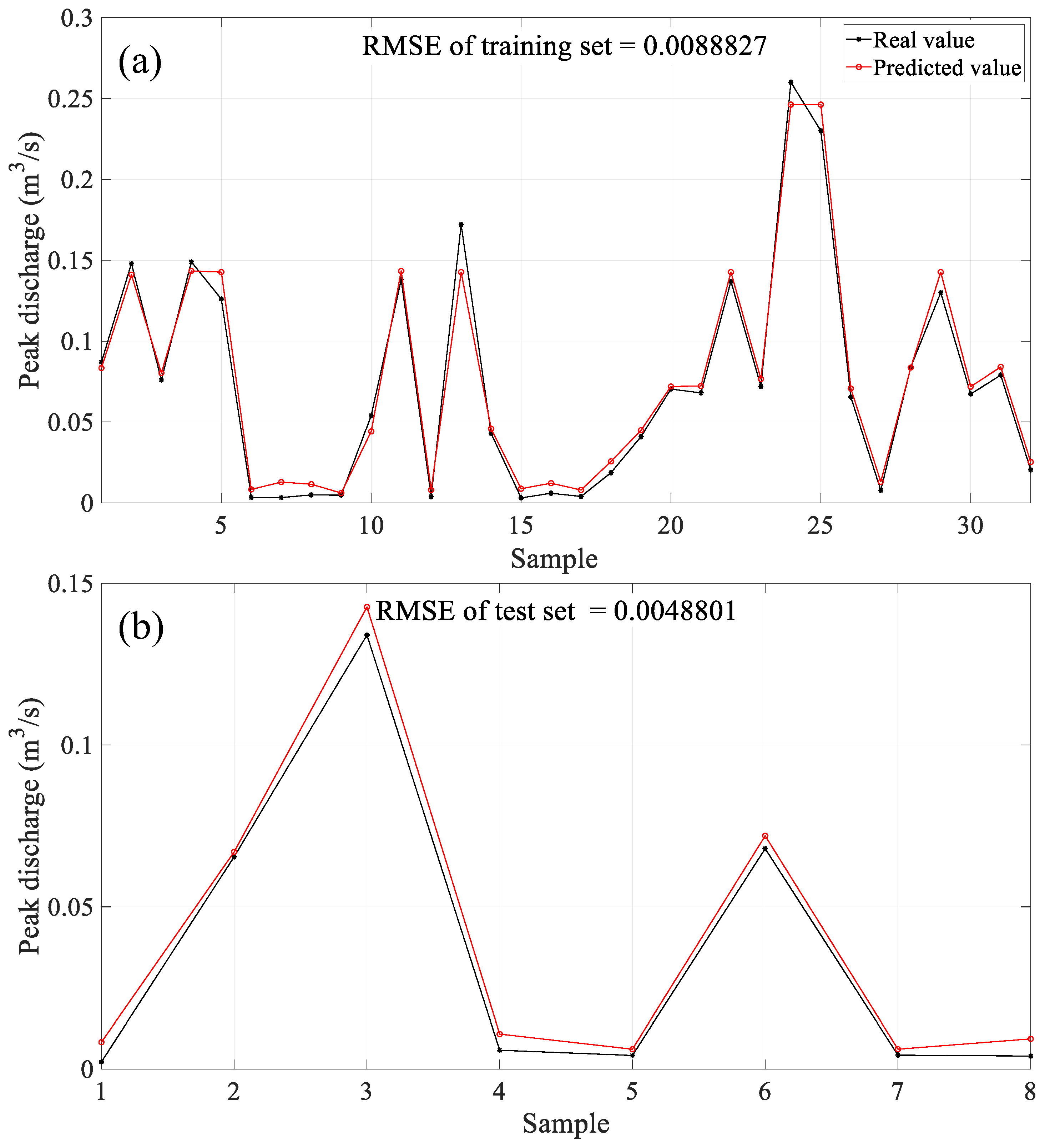
The initial randomness of weights and biases in the network can sometime cause instability of BP, resulting in convergence to a local optimum. To address this issue, the authors introduced a GA [25] into the backpropagation process, enhancing the prediction accuracy. Figure 10 gives the comparisons of the predicted peak discharge and the actual peak discharge, as well as the RMSE. Compared to Figure 8, it is evident that GA-BP exhibits better prediction accuracy qualitatively over BP. The RMSE of the training set and the test set are 0.0088827 and 0.0048801, respectively. For cases with large peak discharges (e.g., case 14, case 18, case 3 in Table 2), the relative errors of GA-BP range from 2.90% to 6.83%, which are one fifth of that produced by BP.
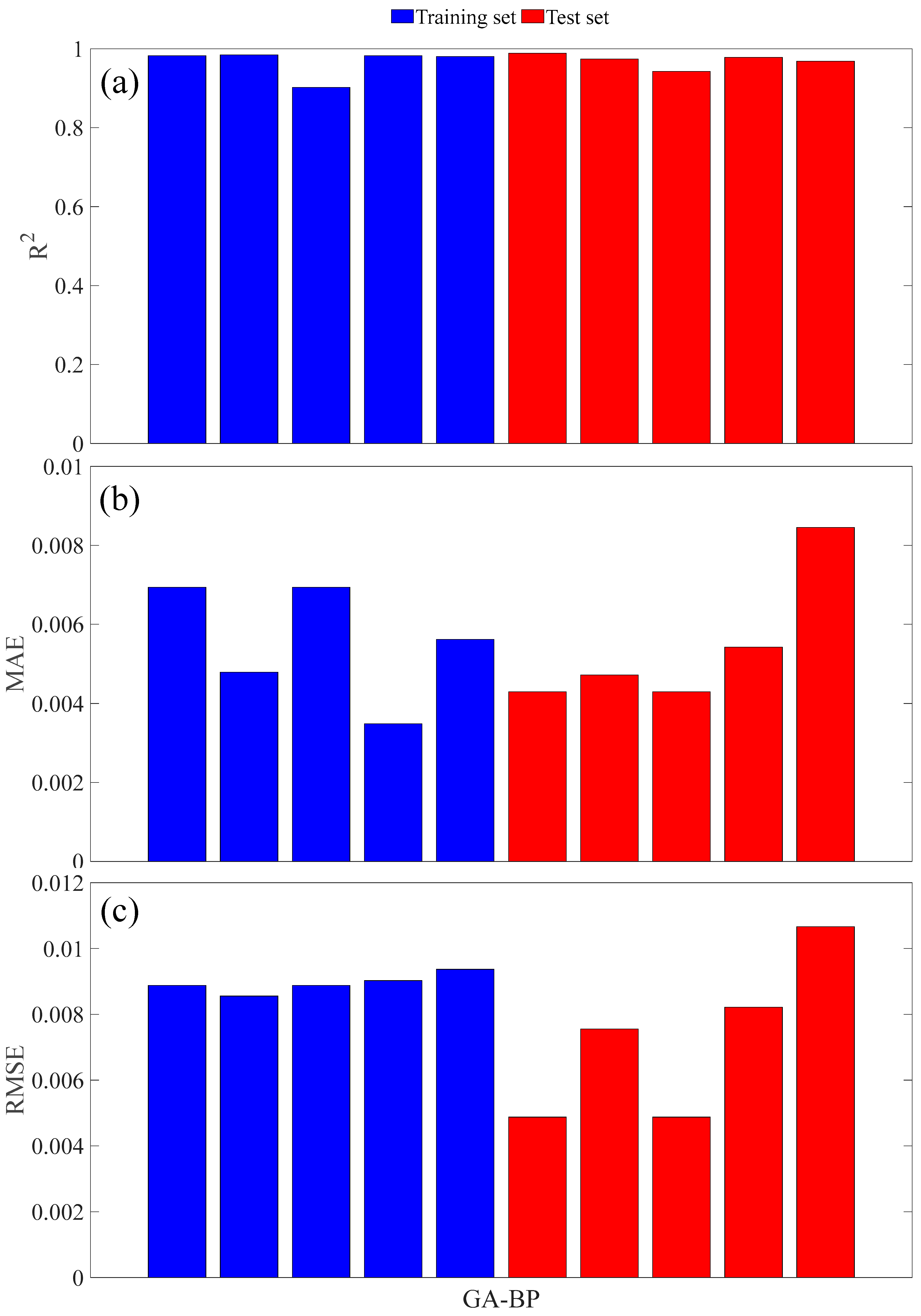
Figure 11 presents the performance evaluation metrics for GA-BP by the five-fold cross-validation. GA-BP performed well across all three metrics, with R2 of the test set exceeding 0.90, indicating that the network exhibited good fitting performance. Additionally, MAE and RMSE were small for all samples. Specifically, the MAE for the test set was lower than that for the training set during the first and third runs, indicating that the network performed efficiently on unseen data. Thus, GA-BP possesses strong generalization capability and good fitting performance.

4.3. Comparison of Peak Discharge between BP and GA-BP

The average performance evaluation metrics for the two networks are given in Table 3, and the optimal results are highlighted in bold. It is worth noting that the R2 of GA-BP is larger, while MAE and RMSE are smaller than that of BP, and these differences are more pronounced on the test set. Compared to BP, the GA-BP shows an average increase of 9.07% in R2, and an average reduction of 57.36% and 57.53% in MAE and RMSE, respectively.
It is essential to be vigilant for overfitting, which occurs when a network performs well on training data but poorly on unseen data. A common approach to detecting overfitting is to compare the performance of the training and test sets using cross-validation results. In this instance, compared to the training set, the R2 of BP for the test set decreases by 7.52%, while GA-BP exhibits an increase of 0.43%. These findings suggest that GA-BP is less susceptible to overfitting and can effectively tackle the challenge of peak discharge prediction.

4.4. Sensitivity Analysis

In this study, the dataset containing nine parameters was created. Nevertheless, these parameters do not have the same contribution to the peak discharge; some of them have minimal influence. Therefore, it is necessary to conduct a sensitivity analysis to quantify the influence of some parameters on the peak discharge.
As suggested by Marangoz et al. [36], Hd, Sc, and P are three dominant parameters on the peak discharge. Three datasets are generated by fixing each dominant parameter. The details of each dataset are listed in Table 4.
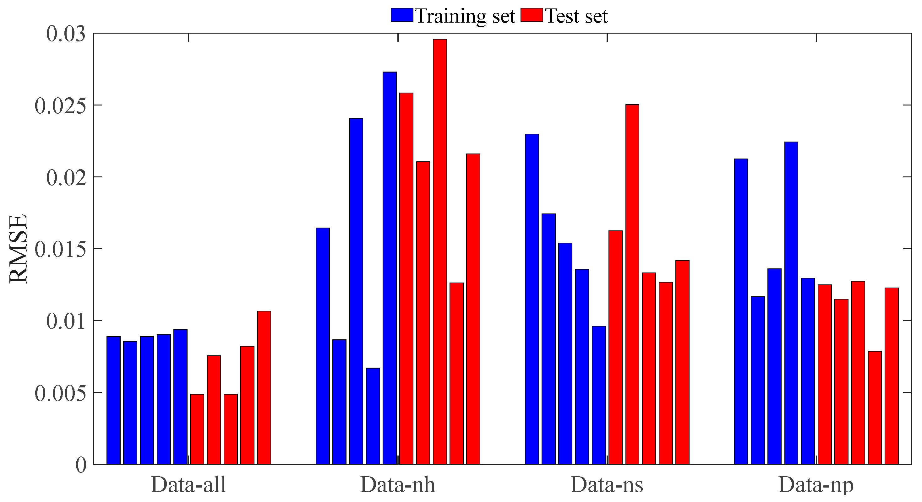
To investigate the effects of three parameters on the prediction of peak discharge, the prediction results obtained from GA-BP on different data sets are compared, as shown in Table 5. The samples in Data-nh keep a constant dam height of 0.46 m. Obviously, the distribution characteristics of the data learned by GA-BP are incomplete as the effects of the dam height are avoided. Because of this, the RMSE is significantly higher on the test set, which represents a real application, with an error improved by 205.81% over Data-all on the test set. The storage capacity of the samples in Data-ns is an invariant (7.38 m3), and the RMSE on the test set is improved by 124.69% compared to that of Data-all. In addition, the RMSE of Data-np (with a constant porosity of 0.5) increases by 57.04%.
The RMSE for each dataset is shown in Figure 12. It is observed in the figure that neglecting the influence of either parameter leads to a greater variability between each prediction and a decrease of the stability, especially in the test set. Considering the accuracy and stability of the prediction models, the dam height has the greatest influence on the peak discharge. The influence of storage capacity and porosity on the peak discharge is not negligible. The sensitivity analyses demonstrate the different effects of each parameter on the peak discharge, which provide a reference for further optimization (e.g., dimensionality reduction) of the prediction model.

5. Discussions

In the previous section, the accuracy of GA-BP in predicting the peak discharge of dam failures was verified. Here, the effectiveness of GA-BP is further discussed by comparing it to some semi-theoretical formulas.
The peak discharge is determined by the shape of the breach-crest cross section, which is strongly associated with the dam configuration [15]. Coleman et al. (2002) proposed a simple estimation of peak discharge based on their experimental data, as Equation (8) [37]:
Q = 3.87 h 3
where h is the water depth in the breach. Walder (2015) also introduced a formula by the combined dimensionless and regression analyses, as Equation (9) [15]:
Q = 5.58 g 0.5 h 2.5
where g is the gravitational acceleration.
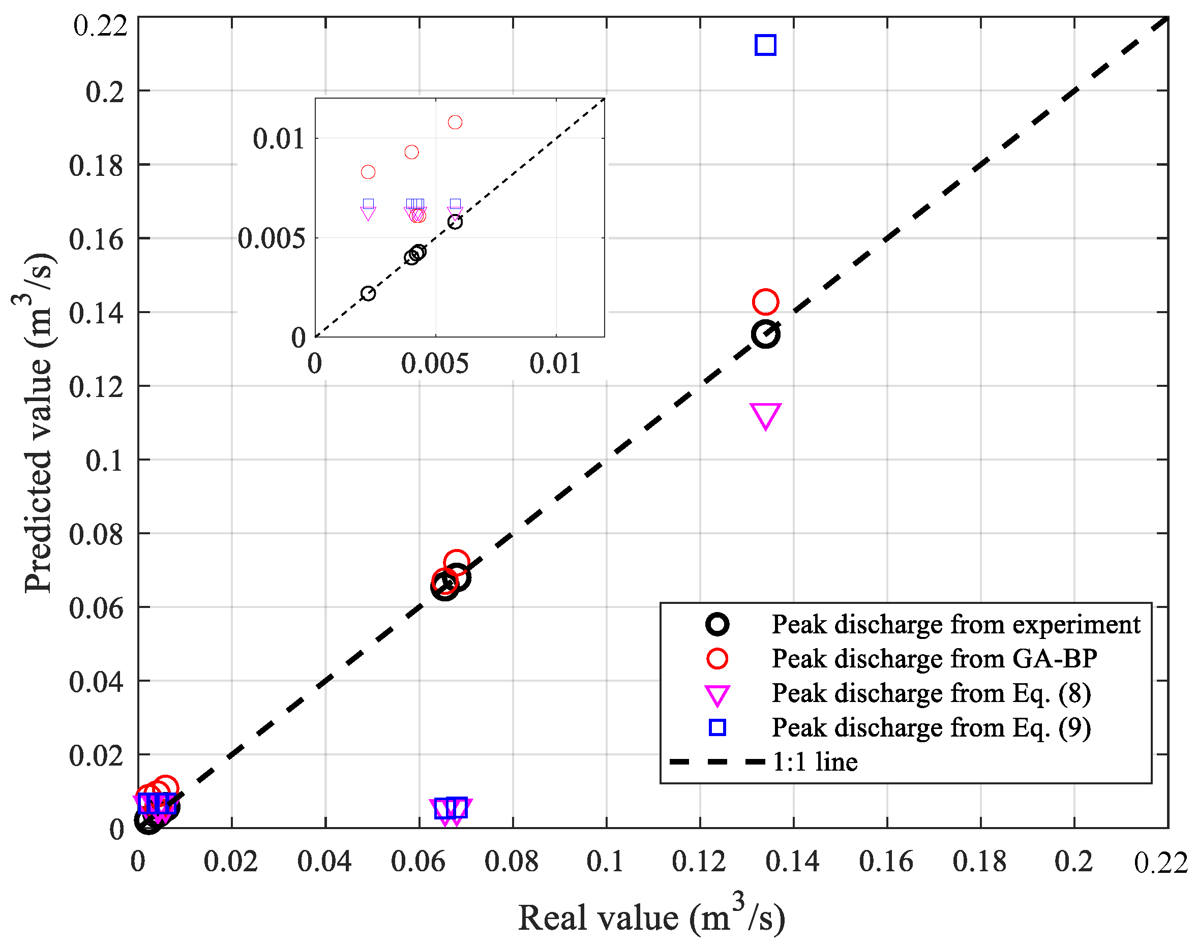
As suggested by Liu et al. [17], h, difficult to estimate accurately, can be assumed to be proportional to H. Then, h in Equation (8) is assumed to be 0.14H, and h in Equation (9) is chosen as 0.4H. The experimental results and that from GA-BP are summarized in Table 6, along with the corresponding results estimated from Equations ((8) and (9)). From this table, that from GA-BP are closer to the experimental results compared to that estimated from Equations ((8) and (9)), particularly when H are 0.2820 m and 0.2788 m. From this figure, the R2, MAE, RMSE of GA-BP are 0.9885, 0.0043, 0.0049, respectively; the R2, MAE, RMSE of Equation (8) are 0.5162, 0.0194, 0.0317, respectively; and that corresponding to Equation (9) are 0.1748, 0.0267, 0.0414, respectively. By comparisons, GA-BP can yield statistically better results than the two semi-theoretical formulas.
The accuracy of GA-BP can also be visualized in the scatter plot as in Figure 13, with each point in this figure representing a predicted value. The black dashed line is a 1:1 line. Therefore, the closer the data points are to this line, the better the prediction. From this figure, the dispersion of data points of GA-BP is much lower than that of Equations ((8) and (9)). In other words, the prediction results of GA-BP are more accurate.

6. Conclusions and Perspective

In this paper, the GA-BP neural network was utilized to predict the peak discharge of dam failures. The GA-BP replaced the traditional backpropagation process in BP with GA operations, including selection, crossover, and mutation. Two networks (BP and GA-BP) were then used to predict the peak discharge. A total of 40 experimental data (14 groups of self-conducted experiments and 26 groups of experiments in literature) were utilized as the samples.
Our results showed that GA-BP outperformed BP in several aspects for the considered dataset: (1) it exhibited an average increase of 9.07% in R2, a 57.36% average reduction in MAE, and a 57.53% average reduction in RMSE; (2) GA-BP demonstrated more accurate results in training and test sets using the five-fold cross-validation method. Overall, the findings indicated that GA-BP was more effective than BP and showed good stability in predicting the peak discharge. Finally, the comparisons between GA-BP and semi-theoretical formulas revealed that GA-BP demonstrates higher accuracy. Sensitivity analysis indicated that dam height (Hd) significantly influences peak discharge.
However, our study has certain limitations. Future research could focus on parameterizing complex dams in practical engineering applications, incorporating additional parameters into the network, and determining the optimal hyper parameters using GA.

Author Contributions

L.R.: Conceptualization, methodology, investigation, writing draft, writing—review and editing; Y.T.: writing draft, writing—review and editing, data curation; J.L.: data curation, investigation; X.J.: writing draft, writing—review and editing; C.F.: writing—review and editing, investigation; X.D.: investigation, writing—review and editing, supervision; H.W.: writing—review and editing, supervision. All authors have read and agreed to the published version of the manuscript.

Funding

This research was funded by the National Natural Science Foundation of China (Grant No. U2342216), the Key R&D Program of the Science & Technology Department of Sichuan Province (Grant No. 2024YFHZ0173), the Ministry of Education Collaborative Education (Grant No. 230806521252005 and 231006521163646), and the second Tibetan Plateau Scientific Expedition by Ministry of Science and Technology (Grant No. 2019QZKK0104).

Data Availability Statement

Data available on request due to restrictions privacy or ethical. The data presented in this study are available on request from the corresponding author.

Acknowledgments

The work was supported, in part, by the Key R&D program of Science & Technology Department of Sichuan Province (Grant No. 2024YFHZ0173), Ministry of Education Collaborative Education (Grant No. 230806521252005), and the second Tibetan Plateau Scientific Expedition by Ministry of Science and Technology (Grant No. 2019QZKK0104).

Conflicts of Interest

We declare that we have no financial or personal relationships with other people or organizations that can inappropriately influence our work. The authors declare that they have no known competing financial interests or personal relationships that could have appeared to influence the work reported in this paper.

Correction Statement

This article has been republished with a minor correction to the Funding statement. This change does not affect the scientific content of the article.

References

  1. Andre, S.; Boillat, J.L.; Schleiss, A. Ecoulements aérés sur évacuateurs en marches d’escalier équipées de macro-rugosités-Partie I: Caractéristiques hydrauliques. La Houille Blanche 2008, 94, 91–100. [Google Scholar] [CrossRef]
  2. Maranzoni, A.; Tomirotti, M. Three-dimensional numerical modelling of real-field dam-break flows: Review and recent advances. Water 2023, 15, 3130. [Google Scholar] [CrossRef]
  3. Selvi, T.; RS, S.S. IoT-Enabled Flood Monitoring System for Enhanced Dam Surveillance and Risk Mitigation. Int. Res. J. Multidiscip. Technovation 2024, 6, 144–153. [Google Scholar]
  4. Tolentino, L.K.S.; Baron, R.E.; Blacer, C.A.C. Real time flood detection, alarm and monitoring system using image processing and multiple linear regression. J. Comput. Innov. Eng. Appl. 2022, 7. [Google Scholar] [CrossRef]
  5. Venkanna, M.P. Floodguard: An IoT-Powered real-time flash flood monitoring and forecasting system. Int. J. Res. Appl. Sci. Eng. Technol. 2024. [Google Scholar] [CrossRef]
  6. Hapuarachchi, H.A.P.; Wang, Q.J.; Pagano, T.C. A review of advances in flash flood forecasting. Hydrol. Process. 2011, 25, 2771–2784. [Google Scholar]
  7. Chang, M.J.; Huang, I.H.; Hsu, C.T.; Wu, S.J.; Lai, J.S.; Lin, G.F. Long-Term Flooding Maps Forecasting System Using Series Machine Learning and Numerical Weather Prediction System. Water 2022, 14, 3346. [Google Scholar] [CrossRef]
  8. Ming, X.; Liang, Q.; Xia, X.; Li, D.; Fowler, H.J. Real-time flood forecasting based on a high-performance 2-D hydrodynamic model and numerical weather predictions. Water Resour. Res. 2020, 56, e2019WR025583. [Google Scholar] [CrossRef]
  9. Antwi-Agyakwa, K.T.; Afenyo, M.K.; Angnuureng, D.B. Know to predict, forecast to warn: A review of flood risk prediction tools. Water 2023, 15, 427. [Google Scholar] [CrossRef]
  10. Wang, H.; Hu, Y.; Guo, Y.; Wu, Z.; Yan, D. Urban flood forecasting based on the coupling of numerical weather model and stormwater model: A case study of Zhengzhou city. J. Hydrol. Reg. Stud. 2022, 39, 100985. [Google Scholar] [CrossRef]
  11. Takayama, S.; Miyata, S.; Fujimoto, M.; Satofuka, Y. Numerical simulation method for predicting a flood hydrograph due to progressive failure of a landslide dam. Landslides 2021, 18, 3655–3670. [Google Scholar] [CrossRef]
  12. Akazawa, F.; Ikeda, A.; Hayami, S.; Harada, N.; Satofuka, Y.; Miyata, S.; Tsutsumi, D. Numerical simulation of landslide dam deformation by overtopping flow. Int. J. Eros. Control Eng. 2014, 7, 85–91. [Google Scholar] [CrossRef]
  13. Hakimzadeh, H.; Nourani, V.; Amini, A.B. Genetic programming simulation of dam breach hydrograph and peak outflow discharge. J. Hydrol. Eng. 2014, 19, 757–768. [Google Scholar] [CrossRef]
  14. Hussain, F.; Wu, R.S.; Wang, J.X. Comparative study of very short-term flood forecasting using physics-based numerical model and data-driven prediction model. Nat. Hazards 2021, 107, 249–284. [Google Scholar] [CrossRef]
  15. Walder, J.S.; Iverson, R.M.; Godt, J.W.; Logan, M.; Solovitz, S.A. Controls on the breach geometry and flood hydrograph during overtopping of noncohesive earthen dams. Water Resour. Res. 2015, 51, 6701–6724. [Google Scholar] [CrossRef]
  16. Al-Riffai, M. Experimental Study of Breach Mechanics in Overtopped Noncohesive Earthen Embankments. Ph.D. Thesis, University of Ottawa, Ottawa, ON, Canada, 2014. [Google Scholar]
  17. Liu, J.; Zhou, C.X.; Chen, W.; Hong, X. Breach discharge estimates and surface velocity measurements for an Earth dam failure process due to overtopping based on the LS-PIV method. Arab. J. Sci. Eng. 2019, 44, 329–339. [Google Scholar] [CrossRef]
  18. Guo, Z.; Leitao, J.P.; Simões, N.E.; Moosavi, V. Data-driven flood emulation: Speeding up urban flood predictions by deep convolutional neural networks. J. Flood Risk Manag. 2021, 14, e12684. [Google Scholar] [CrossRef]
  19. Berkhahn, S.; Fuchs, L.; Neuweiler, I. An ensemble neural network model for real-time prediction of urban floods. J. Hydrol. 2019, 575, 743–754. [Google Scholar] [CrossRef]
  20. Bi, H. Flood and sediment prediction based on BP neural network. South-to-North Water Transfers and Water Science & Technology. South–North Water Transf. Water Sci. Technol. 2015, 13, 406–416. [Google Scholar]
  21. Ye, F.; Kong, X. Prediction of flood level in downstream of the Yellow River based on BP neural network. Open J. Soil Water Conserv. 2022, 10, 41–46. [Google Scholar]
  22. Chen, C.S.; Chen, B.P.T.; Chou, F.N.F.; Yang, C.C. Development and application of a decision group Back-Propagation Neural Network for flood forecasting. J. Hydrol. 2010, 385, 173–182. [Google Scholar] [CrossRef]
  23. He, Y.; Jin, B.; Lv, Q.; Yang, S. Improving BP neural network for the recognition of face direction. In Proceedings of the 2011 International Symposium on Computer Science and Society, Kota Kinabalu, Malaysia, 16–17 July 2011; IEEE: New York, NY, USA; pp. 79–82. [Google Scholar]
  24. Liu, B. Review of swarm intelligence algorithm optimization of BP neural network. Acad. J. Comput. Inf. Sci. 2023, 6, 151–155. [Google Scholar]
  25. Zhang, A.; Sun, G.; Wang, Z.; Yao, Y. A hybrid genetic algorithm and gravitational search algorithm for global optimization. Neural Netw. World 2015, 25, 53–73. [Google Scholar] [CrossRef]
  26. Chak, C.K.; Feng, G. Accelerated genetic algorithms: Combined with local search techniques for fast and accurate global search. In Proceedings of the 1995 IEEE International Conference on Evolutionary Computation, Perth, WA, Australia, 29 November–1 December 1995; IEEE: New York, NY, USA; Volume 1, p. 378. [Google Scholar]
  27. Yu, Q.; Yu, X. An adaptive genetic algorithm based on simulated annealing strategy. In Proceedings of the Third International Conference on Electronic Information Engineering, Big Data, and Computer Technology (EIBDCT 2024), Changchun, China, 22–24 September 2023; SPIE: Bellingham, WA, USA, 2024; Volume 13181, pp. 1221–1227. [Google Scholar]
  28. Liu, J.; He, X.; Huang, H.; Yang, J.; Dai, J.; Shi, X.; Xue, F.; Rabczuk, T. Predicting gas flow rate in fractured shale reservoirs using discrete fracture model and GA-BP neural network method. Eng. Anal. Bound. Elem. 2024, 159, 315–330. [Google Scholar] [CrossRef]
  29. Zhang, L.; Zhang, J.; Ren, P.; Ding, L.; Hao, W.; An, C.; Xu, A. Analysis of energy consumption prediction for office buildings based on GA-BP and BP algorithm. Case Stud. Therm. Eng. 2023, 50, 103445. [Google Scholar] [CrossRef]
  30. Moayedi, H.; Raftari, M.; Sharifi, A.; Jusoh, W.A.W.; Rashid, A.S.A. Optimization of ANFIS with GA and PSO estimating α ratio in driven piles. Eng. Comput. 2020, 36, 227–238. [Google Scholar] [CrossRef]
  31. Rezakazemi, M.; Dashti, A.; Asghari, M.; Shirazian, S. H2-selective mixed matrix membranes modeling using ANFIS, PSO-ANFIS, GA-ANFIS. Int. J. Hydrogen Energy 2017, 42, 15211–15225. [Google Scholar] [CrossRef]
  32. Zhou, J.; Li, C.; Arslan, C.A.; Hasanipanah, M.; Bakhshandeh Amnieh, H. Performance evaluation of hybrid FFA-ANFIS and GA-ANFIS models to predict particle size distribution of a muck-pile after blasting. Eng. Comput. 2021, 37, 265–274. [Google Scholar] [CrossRef]
  33. Li, L.; Gu, Q.; Liu, L. Research on path planning algorithm for multi-UAV maritime targets search based on genetic algorithm. In Proceedings of the 2020 IEEE International Conference on Information Technology Big Data and Artificial Intelligence (ICIBA), Chongqing, China, 6–8 November 2020; IEEE: New York, NY, USA, 2020; Volume 1, pp. 840–843. [Google Scholar]
  34. Zheng, D.; Qian, Z.D.; Liu, Y.; Liu, C.B. Prediction and sensitivity analysis of long-term skid resistance of epoxy asphalt mixture based on GA-BP neural network. Constr. Build. Mater. 2018, 158, 614–623. [Google Scholar] [CrossRef]
  35. Peng, Y.; Xiang, W. Short-term traffic volume prediction using GA-BP based on wavelet denoising and phase space reconstruction. Phys. A Stat. Mech. Its Appl. 2020, 549, 123913. [Google Scholar] [CrossRef]
  36. Marangoz, H.O.; Anılan, T.; Karasu, S. Investigating the non-linear effects of breach parameters on a dam break study. Water Resour. Manag. 2024, 38, 1773–1790. [Google Scholar] [CrossRef]
  37. Coleman, S.E.; Andrews, D.P.; Webby, M.G. Overtopping breaching of noncohesive homogeneous embankments. J. Hydraul. Eng. 2002, 128, 829–838. [Google Scholar] [CrossRef]
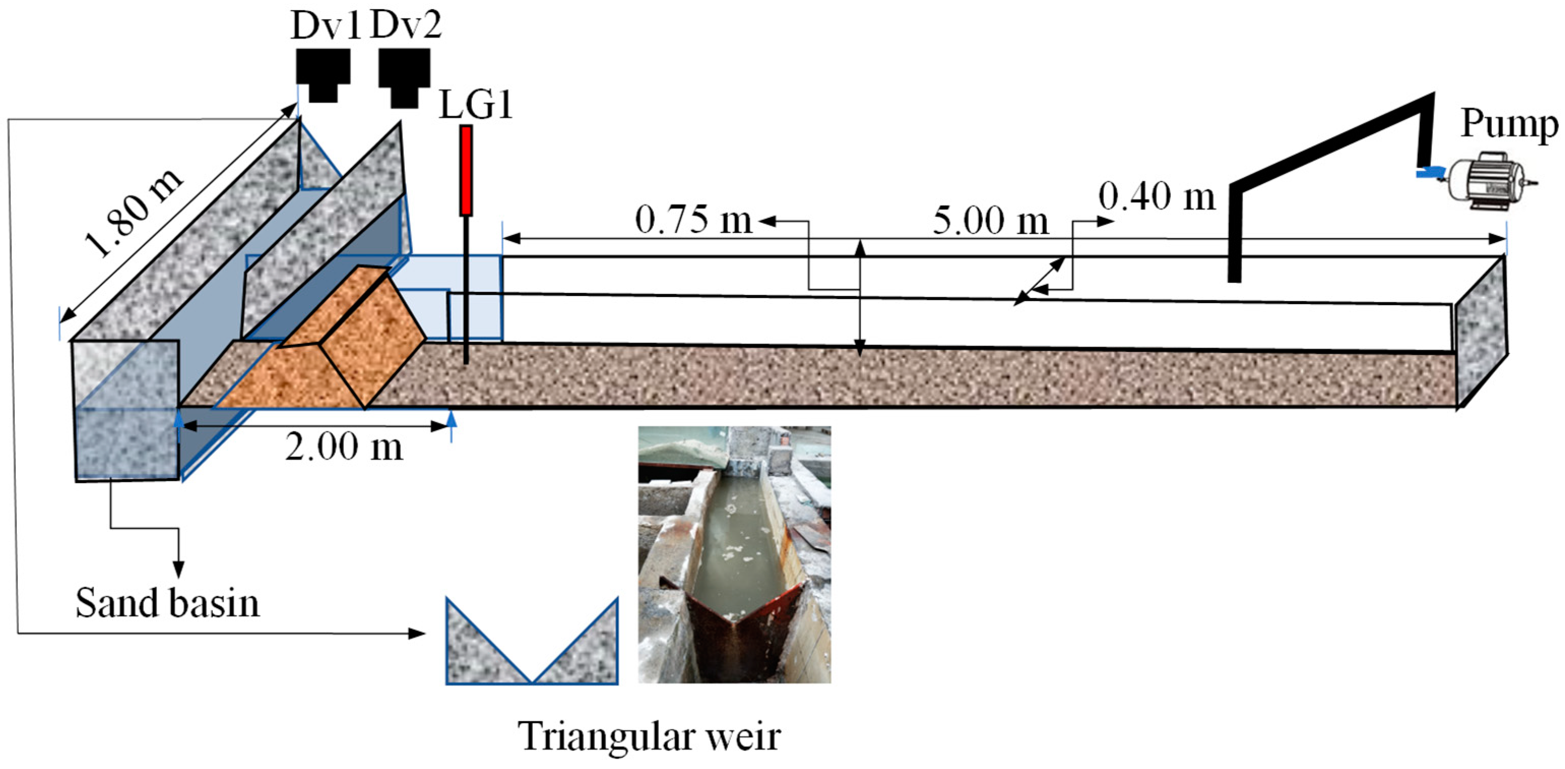
Figure 1. Schematic diagram of dam-failure model and instrument deployment.
Water 16 02946 g001
Figure 2. Experimental site layout.
Water 16 02946 g002
Figure 3. The dam-failure snapshots of test 1 at various instants: (ac) three developing stages of an initial breach at t = 10 s, an expand breach at t = 40 s and a rapid expansion of the breach with collapses at t = 80 s; (df) three decreasing stages of slowing down expansion at t = 120 s, the quasi-steady breach at t = 160 s, and the steady breach at t = 320 s (the ultimate stage).
Water 16 02946 g003
Figure 4. The flow chart of GA.
Water 16 02946 g004
Figure 5. The structure of BP.
Water 16 02946 g005
Figure 6. The iteration flow of weight.
Water 16 02946 g006
Figure 7. The flow chart of GA-BP.
Water 16 02946 g007
Figure 8. Comparisons of the peak discharges between the experimental data and the predicted by BP: (a) training set; (b) test set.
Water 16 02946 g008
Figure 9. The performance evaluation metrics of BP by the five-fold cross-validation: (a) R2; (b) MAE; (c) RMSE.
Water 16 02946 g009
Figure 10. Comparisons of the peak discharges between the experimental data and the predicted by GA-BP: (a) training set; (b) test set.
Water 16 02946 g010
Figure 11. The performance evaluation metrics of GA-BP by the five-fold cross-validation: (a) R2; (b) MAE; (c) RMSE.
Water 16 02946 g011
Figure 12. The performance evaluation metrics for each dataset in five replicate tests.
Water 16 02946 g012
Figure 13. The comparisons of the peak discharges estimated form GA-BP and Equations ((8) and (9)).
Water 16 02946 g013
Table 1. Summary of self-conducted experiment results.
TestDam Height, Hd (m)Crest Width, Lc (m)Base Width, Lb (m)Dam Width, Ld (m)Initial Water Depth, H (m)Median Diameter, D50 (mm)Slotting or NotStorage Capacity, Sc (m3)Porosity, PPeak Discharge, Q (m3/s)
10.300.3001.900.40.302.5No0.56400.5120.0042
20.300.3001.900.40.302.5No0.56400.5120.0043
30.300.3001.900.40.302.5No0.56400.5120.0048
40.300.3001.900.40.302.5Yes0.56400.5120.0040
50.300.2501.750.40.302.5Yes0.56400.5120.0058
60.300.2251.580.40.302.5Yes0.56400.5120.0060
70.300.2251.450.40.302.5Yes0.56400.5120.0078
80.300.2501.600.40.302.5Yes0.56400.5120.0050
90.150.1500.900.40.152.5Yes0.28200.5120.0033
100.200.2001.270.40.202.5Yes0.37600.5120.0034
110.220.2201.390.40.222.5Yes0.41360.5120.0039
120.240.2401.510.40.242.5Yes0.45120.5120.0040
130.300.3001.900.40.302.5Yes0.44400.5120.0031
140.300.3001.900.40.302.5Yes0.32400.5120.0022
Table 2. Available data of dam failures in literatures.
CaseHd (m)Lc (m)Lb (m)Ld (m)H (m)D50 (mm)Slotting or NotSc (m3)PQ (m3/s)Researchers
11.000.3503.5002.00.95000.210Yes12.740.4300.1260Walder (2015) [15]
21.000.3503.5002.00.95000.210Yes12.740.4300.1300
31.000.3503.5002.00.95000.210Yes12.740.4300.1370
41.000.3503.5002.00.95000.210Yes12.740.4300.1720
51.020.3153.5002.00.97000.210Yes12.950.4300.1480
60.761.1553.5002.00.71000.210Yes7.820.4300.0870
70.581.7503.5002.00.53000.210Yes4.600.4300.0410
80.571.7853.5002.00.52000.210Yes4.420.4300.0430
91.000.3503.5002.00.95000.210Yes12.740.4300.1340
100.751.1903.5002.00.70000.210Yes7.620.4300.0720
110.870.7353.5002.00.82000.210Yes10.330.4300.1380
120.870.7353.5002.00.82000.210Yes10.330.4300.1490
130.661.4703.5002.00.61000.210Yes6.080.4300.0540
140.300.1001.7501.50.28720.075Yes11.030.5160.0655Al-Riffai (2014) [16]
150.300.1001.7501.50.28380.075Yes10.860.6060.0680
160.300.1001.7501.50.28190.075Yes10.850.6060.0704
170.300.1001.7501.50.28660.075Yes11.000.7400.0760
180.300.1001.7501.50.28220.075Yes10.840.6060.0673
190.300.0500.8751.50.27880.075Yes5.340.6060.0655
200.300.0330.5831.50.28200.075Yes3.590.6060.0680
210.150.0500.8751.50.14550.075Yes2.750.6060.0205
220.150.0500.8751.50.14280.075Yes2.740.6060.0187
230.100.0110.1941.50.09740.075Yes1.230.6060.0840
240.100.0110.1941.50.09540.075Yes1.220.6060.0790
250.500.5002.5004.00.47000.880Yes44.650.4350.2300Liu et al.
(2019) [17]
260.500.5002.5004.00.47000.880Yes44.650.4350.2600
Table 3. The average performance evaluation metrics of the two networks.
MetricsBP GA-BP
Training SetTest SetTraining SetTest Set
R20.9619780.8896420.9662600.970374
MAE0.0080060.0127410.0055530.005432
RMSE0.0128310.0170470.0089440.007240
Table 4. Details of each dataset generated by combinations of parameters.
DatasetsInvariant ParameterInvariant Parameter Value
Data-all--
Data-nhHd0.46 m
Data-nsSc7.38 m3
Data-npP0.50
Table 5. The average performance evaluation metrics of different datasets.
MetricData-All Data-nh Data-ns Data-np
Training SetTest SetTraining SetTest SetTraining SetTest SetTraining SetTest Set
RMSE0.0089440.0072400.0166310.02214080.015800340.01628720.01638020.01136988
Table 6. Comparisons of the peak discharges among the results from experiment, GA-BP and Equations ((8) and (9)).
H (m)Q (m3/s) from ExperimentQ (m3/s) from GA-BPQ (m3/s) from Equation (8) (with Corresponding h)Q (m3/s) from Equation (9) (with Corresponding h)
0.30000.00220.00830.00630.0067
0.27880.06550.06700.00530.0054
0.95000.1340.14270.11270.2124
0.30000.00580.01080.00630.0067
0.30000.00420.00610.00630.0067
0.28200.0680.07200.00540.0056
0.30000.00430.00610.00630.0067
0.30000.0040.00930.00630.0067
Disclaimer/Publisher’s Note: The statements, opinions and data contained in all publications are solely those of the individual author(s) and contributor(s) and not of MDPI and/or the editor(s). MDPI and/or the editor(s) disclaim responsibility for any injury to people or property resulting from any ideas, methods, instructions or products referred to in the content.