Article

A Water Level Forecasting Method Based on an Improved Jellyfish Search Algorithm Optimized with an Inverse-Free Extreme Learning Machine and Error Correction

1
Power China Huadong Engineering Corporation Limited, Hangzhou 310000, China
2
Faculty of Automation, Huaiyin Institute of Technology, Huaian 223003, China
*
Author to whom correspondence should be addressed.
Water 2024, 16(20), 2871; https://doi.org/10.3390/w16202871
Submission received: 20 September 2024 / Revised: 28 September 2024 / Accepted: 3 October 2024 / Published: 10 October 2024

Abstract

:
Precise water level forecasting plays a decisive role in improving the efficiency of flood prevention and disaster reduction, optimizing water resource management, enhancing the safety of waterway transportation, reducing flood risks, and promoting ecological and environmental protection, which is crucial for the sustainable development of society. This study proposes a hybrid water level forecasting model based on Time-Varying Filter-based Empirical Mode Decomposition (TVFEMD), Inverse-Free Extreme Learning Machine (IFELM), and error correction. Firstly, historical water level data are decomposed into different modes using TVFEMD; secondly, the Improved Jellyfish Search (IJS) algorithm is employed to optimize the IFELM, and subsequently, the optimized IFELM independently forecasts each sub-sequence and obtains the predictive results of each sub-sequence; thirdly, an Online Sequential Extreme Learning Machine (OSELM) model is used to correct data errors, and the initial predictive results and error prediction results are added together to obtain the final prediction for the sub-sequence; and finally, the final prediction for the sub-sequences are added to obtain the prediction results of the entire water level sequence. Taking the daily water level data from 2006 to 2018 in Taihu, China as the research object, this paper compares the proposed model with the ELM, BP, LSTM, IFELM, TVFEMD-IFELM, and TVFEMD-IFELM-OSELM models. The results show that the TVFEMD-IJS-IFELM-OSELM model established in this study has high prediction accuracy and strong stability and is suitable for water level forecasting.

1. Introduction

The rapid advancement of urbanization, coupled with the intensification of the greenhouse effect and the frequent occurrence of extreme weather events due to global warming, has made water level forecasting technology particularly critical in modern society [1,2]. This technology can not only provide early warnings of potential flood disasters to protect people’s lives and property but also provide a scientific basis for the rational allocation and scheduling of water resources by accurately predicting the fluctuations in river water levels. With the development of technologies such as big data and artificial intelligence, water level forecasting models are becoming more accurate and better adapted to complex and variable climatic conditions. The progress of these technologies not only helps us to better understand the impact of climate change on the water cycle but also provides strong scientific support for dealing with climate change, environmental protection, and the rational use of water resources [3,4]. The continuous improvement in water level forecasting technology indicates that it will play a more solid supporting role in the development of human society.
At present, water level forecasting methods are mainly divided into numerical simulation model methods and data-driven model methods. Mohammed et al. [5] conducted GMS numerical simulation modeling and proposed predictive model formulas, thereby establishing a hydrogeological conceptual model for the study area. However, due to the high computational complexity of numerical simulation modeling methods and the poor interpretability and flexibility of the models, which have a large amount of uncertainty, water level prediction research relies more on data-driven models. Li et al. [6] used the Long Short-Term Memory (LSTM) model to analyze and predict the water level of the Three Gorges Reservoir and also analyzed the impact of LSTM variant hybrid models on prediction accuracy. Wang and Tang [7] proposed a water level forecasting model for multi-horizon rivers based on a multi-temporal fusion Transformer, which can effectively adjust the feature weights dynamically, making predictions more informative and practical. Wang and Song [8] proposed a water level forecasting model for stormwater drainage systems based on a Support Vector Machine (SVM), taking the stormwater in Fuzhou City as an example to verify that the SVM has excellent predictive accuracy for water level forecasting. Pan et al. [9] established a water level prediction model based on GRU and CNN, which realized the precise prediction of water level data based on the spatial correlation between water level data. Yan et al. [10] used the Improved Beetle Antennae Search Algorithm to optimize an Extreme Learning Machine (ELM) to predict the water level of the Huibu pump station and Dongsong pump station of the Jiaodong water conveyance project, proving that the ELM model has excellent performance in terms of accuracy and stability in water level prediction. Zhu et al. [11] verified that the Inverse-Free Extreme Learning Machine (IFELM) model shows superior performance compared to the traditional ELM model in time series prediction tasks.
Although many scholars have proposed many mature prediction models and methods, and these models have achieved significant results in prediction effects, there are still some unavoidable problems when using a single model for prediction: the LSTM model requires a large amount of data for training to avoid overfitting, and its complex calculations may lead to suboptimal model performance; the ELM model, although fast in training and good in generalization performance, is very sensitive to data noise. In response to the above problems, some scholars have proposed combined models to improve the accuracy of water level prediction. Guo et al. [12] proposed a Self-Organizing Map–Long Short-Term Memory (SOM-LSTM) combined model for predicting the groundwater level in karst critical zone aquifers, which takes into account the spatial connectivity between observation wells based on geographical multi-feature spatiotemporal correlation and significantly improves the accuracy water level prediction. Hou et al. [13] established a Backpropagation Neural Network–Spatial–Temporal Auto Regressive and Moving Average (BP-STARMA) coupling model, which measures the accuracy of water level prediction from a single model and a coupled model from both time and space perspectives, proving the robustness of the BP-STARMA model. Li et al. [14] established a mixed Singular Spectrum Analysis–Weighted Integration based on Accuracy and Diversity–Group Method of Data Handling–Kernel Extreme Learning Machine (SSA-WIAD-GMDH-KELM) model for river water level forecasting, taking the Xiangjiang River and Yuanjiang River as examples, and verified the high quality of the proposed model.
Due to the nonlinear characteristics of water level data and their inherent instability, directly predicting and analyzing original data may reduce the accuracy of the prediction results [15]. Therefore, many scholars have begun to introduce data decomposition technology as an important part of the water level prediction process [16]. This technology can effectively handle the complexity of water level data, thereby improving the accuracy and reliability of predictions. Cui et al. [17] proposed an ensemble deep learning model for water level prediction combined with quadratic mode decomposition, which processes the data into sub-sequences containing different frequencies through quadratic mode decomposition to achieve high-precision water level prediction. Songhua Huan [18] utilized various decomposition techniques for feature extraction from water quality data and combined sliding correlation and permutation entropy methods to reduce the complexity of the data, thereby eliminating the non-stationary fluctuations in water quality data. This demonstrated that the introduction of decomposition techniques offers higher efficiency than traditional forecasting models. Bai et al. [19] proposed a hybrid model (ICEEMDAN-VMD-WOA-ELM) based on quadratic decomposition and an ELM neural network, which preprocesses the water level dataset with Improved Adaptive Noise Complete Ensemble Empirical Mode Decomposition (ICEEMDAN) and further decomposes the high-frequency sub-sequence Intrinsic Mode Functions obtained by Variational Mode Decomposition (VMD) through quadratic decomposition to achieve high-precision water level prediction.
Although data decomposition technology has performed well in dealing with the nonlinear characteristics, instability, and complex spatiotemporal patterns of water level time series, this method has also led to an expansion in data volume. This expansion directly led to an extension of the model training process, reducing the computational efficiency and potentially causing excessive consumption of computing resources [20]. Therefore, although decomposition technology has its unique advantages in improving prediction accuracy, its demand for computing resources cannot be ignored, and a balance point needs to be found in practical applications.
In response to the above issues, this paper proposes a water level forecasting model called IJS-IFELM-OSELM based on Time-Varying Filter-based Empirical Mode Decomposition (TVFEMD). Firstly, the water level dataset is decomposed through signal decomposition. Compared with traditional EMD, TVFEMD is particularly effective in dealing with nonlinear and non-stationary signals such as water levels. Then, the Improved Jellyfish Search (IJS) algorithm is introduced to optimize the IFELM model. The optimized IFELM model is used to predict the decomposed water level data of Taihu Lake, followed by the use of the Online Sequential Extreme Learning Machine (OSELM) model to correct the errors of the original water level data. Finally, the original predicted values and the error predicted values are superimposed to obtain the final prediction results. This model can significantly improve the convergence speed and prediction accuracy, which is crucial for improving the accuracy and efficiency of water level forecasting. This model can significantly improve the convergence speed and prediction accuracy, which is key to improving the accuracy and efficiency of water level forecasting.
The structure of this paper is as follows: the Section 2 explains the implementation process and working principle of each method proposed in the hybrid model; the Section 3 introduces the source of the water level dataset used in this experiment and the evaluation indicators of the model experiment; the Section 4 elaborates on data processing and the comparison results of the designed model with other commonly used models; and the Section 5 summarizes the methods proposed in this paper and future work; and the Section 6 introduces the limitations of the methods proposed in this paper.

2. Methodology

2.1. Time-Varying Filter-Based Empirical Mode Decomposition

Empirical Mode Decomposition (EMD) [21] is an adaptive signal processing technique that decomposes a complex signal into a set of Intrinsic Mode Functions (IMFs), each representing a different frequency component. Despite its effectiveness, traditional EMD faces certain challenges, such as endpoint effects at the signal boundaries and modal aliasing during the decomposition process, which can compromise the precision and dependability of the outcome [22]. To address these limitations, Li et al. [23] introduced an enhanced approach known as TVFEMD, which aims to mitigate the aforementioned issues.
TVFEMD is an improvement based on EMD. It not only decomposes complex signals into Intrinsic Mode Functions but also solves the problems of modal aliasing and endpoint effects when dealing with wind speed sequences by using non-uniform B-splines as time-varying filters and adaptively designing local cutoff frequencies [24]. This enhances the accuracy of the decomposition and the reliability of signal analysis. The implementation process is as follows:
Perform a Hilbert transform on the input signal σ ( k ) to obtain the transformed signal σ ( k ) * and then calculate its instantaneous amplitude A F ( k ) and instantaneous phase P F ( k ) . The formulas are as follows:
A F ( k ) = σ ( k ) 2 + σ ( k ) 2 *
P F ( k ) = arctan [ σ ( k ) / σ ( k ) * ]
The corresponding analytical signal A(t) is
A ( t ) = σ ( k ) + m σ ( k ) * = A F ( k ) e m P F ( k )
Interpolate based on the local upper and lower bounds of A F ( k ) to obtain curves τ 1 ( k ) and τ 2 ( k ) ; the corresponding amplitudes are presented as λ 1 ( k ) and λ 2 ( k ) :
λ 1 ( k ) = τ 1 ( k ) + τ 2 ( k ) 2
λ 2 ( k ) = τ 1 ( k ) τ 2 ( k ) 2
Interpolate the upper and lower limits of A F 2 ( k ) to obtain γ 1 ( k ) and γ 2 ( k ) and calculate the instantaneous frequency components σ 1 * ( k ) and σ 2 * ( k ) :
σ 1 * ( k ) = γ 1 ( k ) 2 λ 1 2 ( k ) 2 λ 1 ( k ) λ 2 ( k ) + γ 2 ( k ) 2 λ 1 2 ( k ) + 2 λ 1 ( k ) λ 2 ( k )
σ 2 * ( k ) = γ 1 ( k ) 2 λ 2 2 ( k ) 2 λ 1 ( k ) λ 2 ( k ) + γ 2 ( k ) 2 λ 2 2 ( k ) + 2 λ 1 ( k ) λ 2 ( k )
Local cutoff frequency σ bis * ( k ) calculation can be carried out as follows:
σ bis * ( k ) = σ 1 * ( k ) + σ 2 * ( k ) 2
Signal φ ( k ) = cos [ σ bis * ( k ) d ( k ) ] , using φ ( k ) as the local extremum points as nodes, employs a B-spline approximate filter to further interpolate τ ( k ) , resulting in the filtered outcome C 1 ( k ) .
If θ ( k ) = B L ( k ) / σ avg ( k ) ζ = 0.1 , then σ ( k ) is taken as a component of an IMF; otherwise, σ ( k ) C 1 ( k ) is taken as the new input signal, and the above steps are repeated. ζ is the bandwidth threshold, σ avg ( k ) is the weighted mean instantaneous frequency, and B L ( k ) is the instantaneous bandwidth.
Ultimately, the original input signal σ ( k ) , after decomposition by TVFEMD, yields S sub-sequences C i ( k ) | i = 1 , 2 , , S , where C i ( k ) is the i-th sub-sequence, and it simultaneously satisfies the following:
σ ( k ) = i = 1 S C i ( k )

2.2. Jellyfish Search Algorithm

2.2.1. Standard Jellyfish Search Algorithm

The Jellyfish Search Algorithm (JS) [25] is an optimization algorithm that simulates the foraging behavior of jellyfish. The basic idea is to imitate the way jellyfish drift and feed randomly in the ocean, searching for optimal solutions through a process of random wandering [26].
The first step involves initializing the jellyfish population with a population size of N and a maximum number of iterations of M ax n . The upper and lower bounds of the search space are U b and L b , respectively. The Logistic chaotic map is used to generate the initial jellyfish population. The Logistic map is as follows:
E i + 1 = η E i ( 1 E i ) , 0 E 0 1
where E i is the Logistic chaos value of the position of the jellyfish, with i taking values in the range of { 1 , 2 , , N } , and E 0 is the initial value of the Logistic map, E 0 { 0.0 , 0.25 , 0.5 , 0.75 , 1.0 } , η = 4 .
The movement patterns exhibited by jellyfish vary at different times; hence, a time control mechanism is introduced to transition between movement modes. The formula for the time control function is
F t = ( 1 t M a x n ) × ( 2 × r a n d ( 0 , 1 ) 1 )
Ocean currents contain a wealth of nutrients that attract a large number of jellyfish to move along with them. If F ( t ) < 0.5 , the jellyfish move with the current. The position update formula is
E i ( t + 1 ) = E i ( t ) + r a n d ( 0 , 1 ) × ( E best β × r a n d ( 0 , 1 ) × μ )
where E i ( t ) is the position of the i-th jellyfish, E best is the best position among the current jellyfish population, β is the distribution coefficient with β = 3 , and μ is the average position of all jellyfish in the population.
When F ( t ) < 0.5 and rand ( 0 , 1 ) > ( 1 F ( t ) ) , the jellyfish undergo passive movement, and the position update formula is
E i ( t + 1 ) = E i ( t ) + γ × r a n d ( 0 , 1 ) × ( U b L b )
where γ > 0 is the movement coefficient, taking the value of γ = 0.1 .
When F ( t ) < 0.5 and rand ( 0 , 1 ) ( 1 F ( t ) ) is the condition met, the jellyfish engage in active movement, and the position update formula is
E i ( t + 1 ) = E i ( t ) + r a n d ( 0 , 1 ) × D i r e c t i o n
where D i r e c t i o n represents the movement direction within the group, denoted as D i r e c t i o n = E j ( t ) E i ( t ) , f ( E i ) f ( E j ) E i ( t ) E j ( t ) , f ( E i ) < f ( E j ) , E j ( t ) is the position of a jellyfish randomly selected from the t-th generation population ( j i ) , and f ( E i ) and f ( E j ) are the fitness values of the i-th and j-th jellyfish, respectively.

2.2.2. Optimized Jellyfish Search Algorithm Based on Tent Map

The Tent map generates a chaotic sequence to initialize the jellyfish population. To ensure that the initial solutions are more uniformly distributed in the solution space, a good initial population helps with the convergence speed and accuracy of the algorithm.
z i + 1 = 2 z i , 0 z 0.5 2 ( 1 z i ) , 0.5 < z i 1
where z i represents the function value obtained after the i-th transformation, where i denotes the number of transformations. Starting from the initial value z 0 , a sequence is generated according to the given formula until a predetermined goal is reached.
Additionally, an adaptive weight mechanism is introduced to simulate the jellyfish moving with ocean currents and continuously adjusting their positions. As iterations progress, the weight factor ω will change linearly. In the early stages of the algorithm, a larger weight coefficient makes the algorithm more inclined to conduct a global search, and as the iterations deepen, the weight coefficient gradually decreases, causing the search focus to gradually concentrate on a specific area. This strategy helps the algorithm avoid becoming stuck in local optima, thereby improving the accuracy of the solution. The position update formula for the jellyfish is as follows:
E i ( t + 1 ) = ω   E i ( t ) + r a n d ( 0 , 1 ) × ( E best β × r a n d ( 0 , 1 ) × μ )
ω ( t ) = e t M a x n u
where t represents the current iteration count; M ax n represents the maximum number of iterations; and u represents a modulation coefficient, the purpose of which is to adjust the magnitude of the weight factor.

2.3. The Extreme Learning Machine and Its Improved Versions

2.3.1. Extreme Learning Machine

The ELM [27] is a machine learning algorithm. It mainly consists of an input layer, a hidden layer, and an output layer. Due to its simplicity and efficiency, it has a fast training speed when processing large-scale data [28].
The output of the hidden layer W c is represented as
W c = w 1 b w 2 b w U b
w j b = H q j b + h j
In the formula, w j b represents the output of the j-th hidden node, b is the input variable, and j = 1 , 2 , , U , where U denotes the number of neurons in the hidden layer, is the Sigmoid activation function, h j indicates the bias at the hidden node, and q j is the weight value at the hidden node.
The output expression of the Extreme Learning Machine is given by
o u t = i = 1 o j y ( q j X m + ν j ) , m = 1 , 2 , , O
where O represents the number of samples in the training set, ν j represents the bias of the j-th input node and hidden layer node, o u t indicates the weight value connecting the j-th hidden node to the output layer, and j denotes the output value of the j-th hidden node.
The ELM is a method designed for training single-layer feedforward neural networks. It initiates with randomly assigned weights and biases for the input to the hidden layer, subsequently determining the weights for the output layer. The process involves optimizing a loss function that includes both the training error and a regularization component based on the norm of the output weights. This optimization leverages the properties of the Moore–Penrose pseudoinverse. In the past ten years, the principles and applications of the ELM have been extensively explored. In terms of training efficiency, the ELM is recognized for its minimal training parameters, swift training process, and robust generalization. Nonetheless, it faces challenges such as the need for parameter optimization, which requires iterative experimentation to tailor the settings for specific problems.

2.3.2. Inverse-Free Extreme Learning Machine

The IFELM [29] is a machine learning method that incrementally increases the number of hidden layer nodes and optimally updates the weight values step by step.
Assuming an ELM with l hidden layer nodes, and with an additional hidden layer node added, the output weights at this time are represented as
W T ( l + 1 ) = w l + 1 1 w l + 1 2 w l + 1 U U T
The input bias is represented as b l + 1 . At this point, the output of the hidden layer is represented as
J l + 1 = J l s l + 1 T
In the formula, J l represents the output of an ELM with l hidden layer nodes.
An inverse-free algorithm is used to update the regularized pseudo-inverse to avoid inverse operations during the weight update process. The method of operation is as follows:
G = J T J J T + L 0 2 D 1
After iteratively computing G l + 1 = G ˜ l g ¯ l + 1 , the calculation method for G ˜ l is as follows:
G ˜ l = s l + 1 T s l + 1 + L 0 2 D s l + 1 s l + 1 T G l J l s l + 1 s l + 1 T G l s l + 1 T s l + 1 + L 0 2 s l + 1 T s l + 1 + L 0 2 s l + 1 T G l J l s l + 1    + s l + 1 T s l + 1 + L 0 2 D s l + 1 s l + 1 T G l s l + 1 T s l + 1 + L 0 2
The calculation method for g ¯ l + 1 is as follows:
g ¯ l + 1 = G ˜ l J l s l + 1 s l + 1 T s l + 1 + L 0 2 + s l + 1 s l + 1 T s l + 1 + L 0 2
Let I = J J T + L 0 2 D be defined; then, I l + 1 = J l + 1 J l + 1 T + L 0 2 D l + 1 is determined, and by substituting it into equation J l + 1 we obtain
I l + 1 = I l J l s l + 1 J l s l + 1 T s l + 1 T s l + 1 + L 0 2

2.3.3. Online Sequential Extreme Learning Machine

OSELM [30] is an extension of the ELM, designed as an incremental learning algorithm that specifically handles data arriving in sequential batches. The OSELM inherits the fast training speed and strong generalization capabilities of the ELM and has the added ability to dynamically update model parameters based on the latest data [31]. This algorithm gradually integrates new information, enabling the model to adapt to changes in data streams, thereby maintaining or enhancing its performance during the continuous learning process. The training process of the OSELM mainly consists of two stages.
In the first part, the initialization phase, it is assumed that there are N * training samples ( S R i , S C i ) , where S R i = S R i 1 , S R i 2 ,   ,   S R i n T represents the input values of the model and S C i = S C i 1 , S C i 2 ,   ,   S C i n T represents the model’s desired output values. Using the traditional ELM (Extreme Learning Machine) model, the minimum value β 0 is calculated while satisfying the condition H * β T 0 . The process typically involves the following steps:
H * = S i g m o i d q 1 * , h 1 , S R 1 S i g m o i d q N * , h N , S R 1 S i g m o i d q 1 * , h 1 , S R N 0 S i g m o i d q N * , h N , S R N 0 N 0 × N
where q * represents the weights between the input layer and the hidden layer.
Following this, the least squares method, combined with the concept of the Moore–Penrose pseudoinverse, is used to determine the hidden layer weights, A. The process typically involves the following steps:
β 0 = H * T T 0 1 H * T T 0
The second part is the online learning phase, where when new samples enter the model, the output weights are derived using the online learning recursive formula. The process typically works as follows:
β ( k + 1 ) = β ( k ) + ( H * T T k + 1 ) 1 H * T ( T k + 1 H * β ( k ) )

2.4. Error Correction

After the preliminary prediction by the IFELM, a prediction error is generated. Since the water level data error series is a signal with overlapping multi-spectrum, it has characteristics of non-stationarity and nonlinearity. To overcome the error caused by the multi-scale spectral superposition of the error series, this paper decomposes it through TVFEMD. On this basis, the decomposed sub-sequences of different frequencies are modeled separately by the IFELM. Finally, the predicted results of different sub-sequences are integrated to obtain the error prediction value. The process of error correction is shown in Figure 1.
Initially, the water level time series is subjected to TVFEMD for decomposition into its constituent components. Subsequently, each of these components undergoes a preliminary prediction phase using the IFELM. The difference between the actual water level measurements and the preliminary predictions is calculated to determine the error in the water level time series. The mathematical expression for this process is provided below:
E r r o r c = O v a l u e c I v a l u e c
where E r r o r c represents the error value of the water level data at time c, O v a l u e c denotes the actual measured value at time c, and I v a l u e c indicates the initial predicted value at time c.
By utilizing the obtained water level data error time series as restructured input, the OSELM time series model predicts the error at time c, E r r o r c , using data from times prior to c. This process results in the predicted error outcome for the water level data at time c, denoted as I E r r o r c .
The initial predicted result is added to the error prediction result to obtain the final prediction outcome. The formula is as follows:
F v a l u e c = I v a l u e c + I E r r o r c
where F v a l u e c represents the final water level prediction value at time c.

2.5. Construction of Water Level Forecasting Model

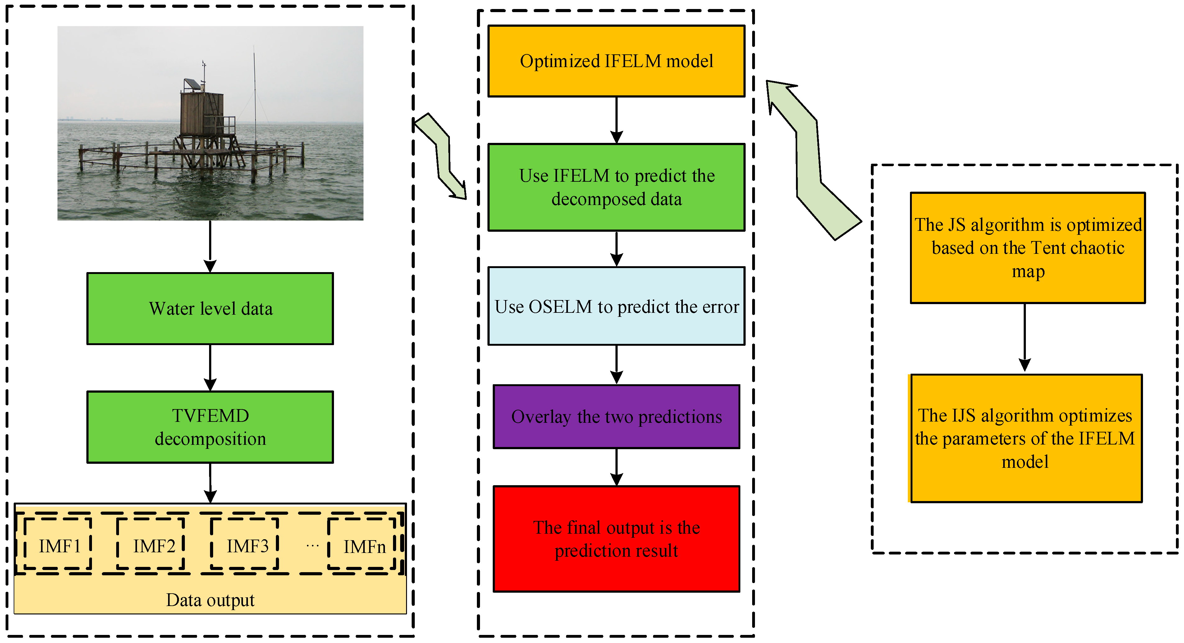
The TVFEMD-IJS-IFELM-OSELM hybrid forecasting model established in this paper is specifically constructed as shown in Figure 2. Firstly, TVFEMD is used to decompose complex historical water level data into several stable sub-sequences that are easier to analyze and predict without changing the nature of the original time series. Then, the optimized IJS algorithm is employed to optimize the IFELM model. Subsequently, the decomposed data are used as input for the optimized IFELM to make predictions, ultimately yielding the output forecast results. The specific steps are as follows:
(1)
First, the historical water level data are selected from the Taihu and the TVFEMD method is used. The vector obtained from the decomposition of the historical water level single-variable data is denoted as X1, and its specific representation is as follows:
X 1 = I M F 1 I M F 2 I M F n
In the formula, n represents the number of components obtained after TVFEMD.
(2)
The first 80% of the steady-state components are set as the training set. Taking the historical water level data of 13 years, totaling 4557 days, as the overall observed values, the water level data of the previous 10 days are used to predict the water level value of the 11th day to achieve a 1-day water level forecast. Taking the i-th (i = 1, 2, …, t) component after decomposition as an example, the input model dataset I M F X i and the corresponding output I M F Y 1 i are
I M F X i = x 1 i x 2 i x D d i x 2 i x 3 i x D d + 1 i x d i x d + 1 i x D 1 i
I M F Y 1 i = x d + 1 i x d + 2 i x D i
(3)
Utilizing the IJS algorithm to optimize the IFELM model, the input I M F X i and output I M F Y i data obtained from Step (2) are divided into training and testing datasets, which then serve as inputs for the optimized IFELM model. The model is trained and used to predict the testing data, yielding water level forecast values. Subsequently, the OSELM model is employed to correct the errors in the original water level data, resulting in corrected forecast values. Finally, the water level predictions and the error-corrected values are superimposed to obtain the final forecast values, as shown in Figure 2.
(4)
To verify the performance of the model, ELM (Extreme Learning Machine), BP (Backpropagation), LSTM (Long Short-Term Memory), IFELM (Inverse-Free Extreme Learning Machine), TVFEMD-IFELM, and TVFEMD-IFELM-OSELM are set as comparative models. The model’s credibility is assessed using the Root Mean Square Error (RMSE), Mean Absolute Error (MAE), Mean Absolute Percentage Error (MAPE), and Nash Efficiency Coefficient/Coefficient of Determination (NSE) as the evaluation criteria for model performance.
In the process of conducting the aforementioned analysis, MATLAB software was utilized for the mathematical computation and visualization of the TVFEMD-IJS-IFELM-OSELM model, enabling the implementation of its construction, training, prediction, and performance evaluation.

3. Watershed Introduction and Evaluation Indicators

3.1. Watershed Introduction

The Taihu Basin, located in the eastern part of China, is an important component of the Yangtze River Delta, covering parts of the Jiangsu and Zhejiang provinces. This basin is known for its abundant water resources, with Taihu itself being the largest lake within the basin, playing a key role in maintaining ecological balance and supporting regional economic activities. The river network in the Taihu Basin is well developed, including major rivers such as Suzhou River and Huangpu River, which are connected to Taihu, forming a complex water system. These rivers not only provide water sources for agricultural irrigation but are also important sources of water for industry and domestic use.
Situated in the heart of the Taihu Basin within Wuxi, Jiangsu Province, the Taihu Basin monitoring station plays a pivotal role in the surveillance and documentation of the region’s hydrological data. This includes vital metrics such as water levels and flow rates. The collected data are instrumental for the management of water resources, the mitigation of flood risks, and the preservation of ecological and environmental health within the basin. By analyzing these data, authorities can promptly assess the status of Taihu’s water resources, devise well-informed strategies for their sustainable use and conservation, and thus safeguard the long-term viability of the Taihu Basin.

3.2. Evaluation Metrics

Data prediction evaluation metrics are essential tools for assessing the performance and effectiveness of forecasting models. In this paper, the Root Mean Square Error (RMSE), Mean Absolute Error (MAE), Mean Absolute Percentage Error (MAPE), and Nash–Sutcliffe Efficiency Coefficient (NSE) are used to quantify the discrepancy between the forecast results and actual observations as well as the model’s fit. Detailed definitions of these evaluation metrics and their corresponding calculation methods are specifically displayed in Table 1 of the text.
In Table 1, y i represents the true observed values; y ^ i represents the model’s predicted values; y ¯ represents the mean of the observed values; and n represents the number of samples. These evaluation metrics can assess the accuracy and fit of the TVFEMD-IJS-IFELM-OSELM forecasting model in the prediction of water levels in Taihu.

4. Experimental Results and Case Studies

4.1. Data Preprocessing

The decomposition results of the TVFEMD algorithm are shown in Figure 3. Under the decomposition of the TVFEMD algorithm, the Taihu water level time series is decomposed into five IMFs I M F 1 , I M F 2 , , I M F 5 . Compared with other components, I M F 1 I M F 4 has a higher frequency, showing strong randomness and volatility. I M F 5 shows a slow trend with significantly reduced volatility, and the waveform is close to a sine wave. The IMF components of the Taihu water level time series decomposed by the TVFEMD algorithm gradually decrease in frequency, increase in regularity, decrease in discreteness, and gradually stabilize the trend, reflecting the characteristics and patterns of Taihu’s daily water level changes from 2006 to 2018.

4.2. Comparative Experimental Design and Result Analysis

Table 2 presents the predictive performance of seven different models for forecasting water levels one day ahead: the ELM, Backpropagation (BP), Long Short-Term Memory network (LSTM), IFELM, TVFEMD-IFELM, the combination of Inverse-Free Extreme Learning Machine with Online Sequential Extreme Learning Machine based on Time-Varying Filter Experience Mode Decomposition (TVFEMD-IFELM-OSELM), and the combination of the Improved Jellyfish Search Algorithm optimized with an Inverse-Free Extreme Learning Machine with an Online Sequential Extreme Learning Machine based on Time-Varying Filter Experience Mode Decomposition (TVFEMD-IJS-IFELM-OSELM). The experimental setup for model parameters is detailed as follows: The LSTM configuration includes 30 neurons in the input layer, 60 in the hidden layer, a minimum batch size of 1, a single neuron in the output layer, a maximum of 2000 training epochs, and a learning rate of 0.001. The BP model is configured with up to 2000 training epochs, a learning rate of 0.001, and an error threshold of 0.00001. The ELM model comprises 30 neurons in the input layer and 120 in the hidden layer. The IFELM model features a regularization coefficient of 1000 and employs the Sigmoid activation function, with 30 neurons in the input layer and 120 in the hidden layer. The OSELM model is characterized by a regularization coefficient of 1000, 30 input neurons, 120 hidden neurons, a forgetting factor of 0.95, and a learning rate of 0.01.
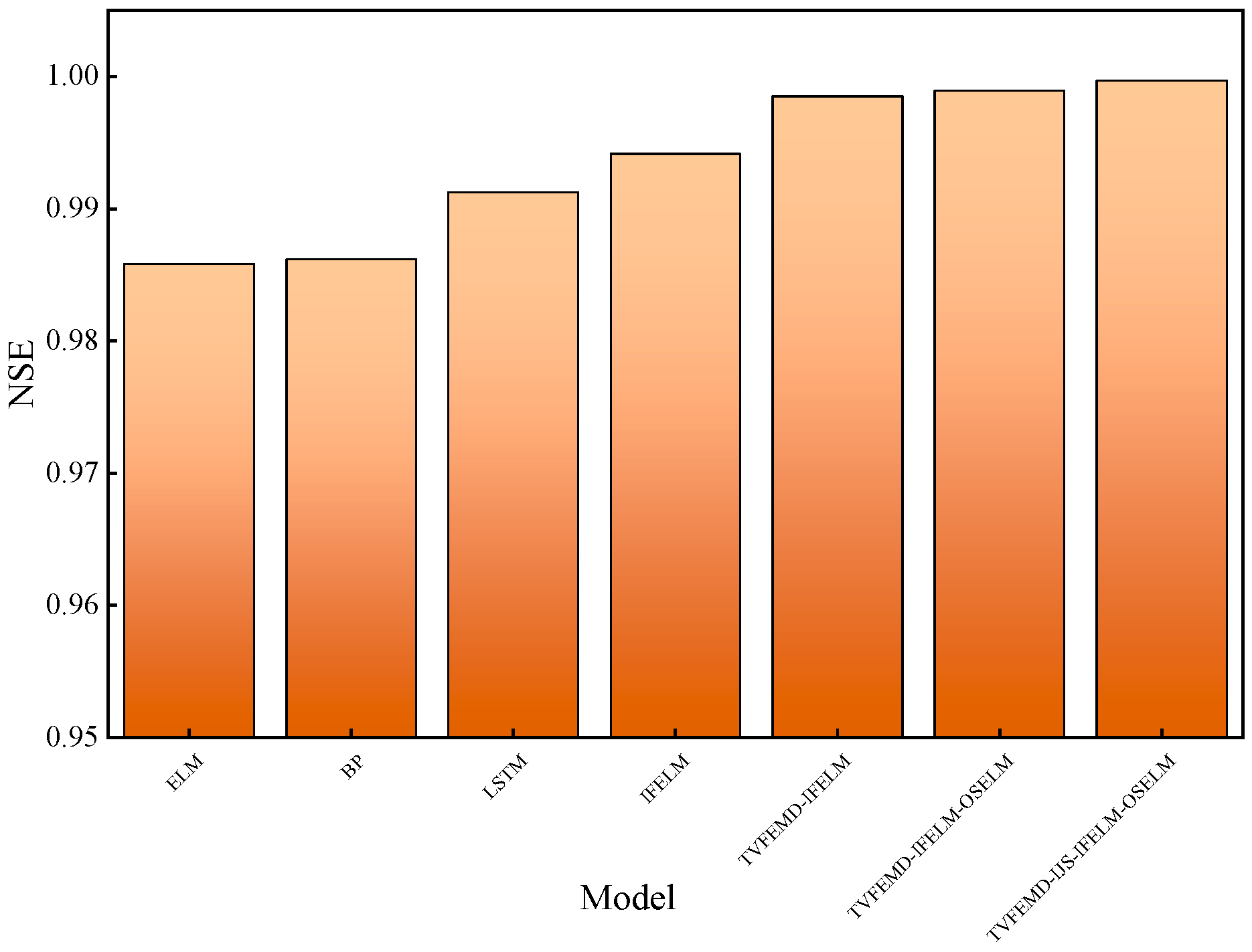
From Table 2, it can be observed that the NSE of the forecasting models ELM, BP, LSTM, IFELM, TVFEMD-IFELM, TVFEMD-IFELM-OSELM, and TVFEMD-IJS-IFELM-OSELM gradually improves, with the proposed model showing the best effect, and its NSE indicator is significantly higher than that of the other models. According to the data indicators in the table, since TVFEMD was added to decompose the input data of IFELM, the overall forecasting effect of the TVFEMD-IFELM combined model is slightly better than that of RELM. After the error correction was added, the overall forecasting accuracy of the model was further improved, making the advantage of the TVFEMD-IFELM-OSELM combined model more obvious than that of the TVFEMD-IFELM combined model. On the basis of the TVFEMD-IFELM-OSELM combined model, after the IJS algorithm was introduced to improve and reorganize the parameters of the IFELM to obtain the TVFEMD-IJS-IFELM-OSELM combined model, the indicators in Table 2 show that in the 1-day-ahead forecast, the RMSE, MAE, and MAPE indicators of the TVFEMD-IJS-IFELM-OSELM combined model are all better than those of the TVFEMD-IFELM-OSELM combined model and were improved by 0.49%, 0.12%, and 0.03%, respectively. In addition, in the 1-day-ahead forecast, the NSE indicator of the TVFEMD-IJS-IFELM-OSELM combined model is the best among all compared models and was improved by 0.08% compared to the TVFEMD-IFELM-OSELM combined model. Moreover, in hydrology and environmental science, the reference significance of the NSE indicator is relatively greater.
Figure 4 presents a comparison of the NSE for the proposed model and the control group models in predicting the water level one day ahead. It can be observed from Figure 4 that the Nash Efficiency Coefficient of the proposed model is higher than that of the other models.
By employing a well-trained model, we predicted the daily water levels of Taihu for the period from 2016 to 2018. These predictions were then compared against the actual observed values, revealing a satisfactory correlation. Figure 5 presents the fit line charts of various control models for forecasting the water level one day in advance, spanning the years 2016 to 2018.
Figure 6 presents the error line charts comparing the predicted values with the observed values for the BP, ELM, LSTM, IFELM, TVFEMD-IFELM, TVFEMD-IFELM-OSELM, and TVFEMD-IJS-IFELM-OSELM models. It can be seen that the TVFEMD-IJS-IFELM-OSELM model has the smallest fluctuation in the difference between the predicted results and the observed values. Therefore, it is concluded that the model proposed in this paper has more accurate predictions with the smallest deviation from the observed values compared to the other models.
Table 3 presents the peak water level forecast results and error table for one-day-ahead predictions by various models, showing the forecast outcomes for the six-year peak water levels contained in the testing dataset and the corresponding errors, with the six errors then averaged. According to the data in the table, the proposed TVFEMD-IJS-IFELM-OSELM forecasting model exhibits some fluctuation in the peak water level predictions for certain years, but it demonstrates an absolute advantage in terms of the average error.
Figure 7 presents the scatter plots for the IFELM, TVFEMD-IFELM, TVFEMD-IFELM-OSELM, and TVFEMD-IJS-IFELM-OSELM forecasting models. It can be observed from the figure that, compared to the other three models, the TVFEMD-IJS-IFELM-OSELM model has the highest degree of scatter aggregation and the best fit for the prediction results. Therefore, the hybrid model proposed in this paper offers higher accuracy in water level forecasting, better captures the nonlinear relationships between historical water level data, and is able to more accurately predict future trends in water levels.

5. Conclusions

This article uses historical water level prediction for Taihu as a case study and draws the following conclusions through experimental research:
(1)
The original water level data exhibit low regularity. By introducing the TVFEMD algorithm to decompose the original sequence, the complex original sequence is broken down into simpler sub-sequences, which improves the computational efficiency and, at the same time, enhances the accuracy of prediction.
(2)
By employing the TVFEMD technique, the original water level data are decomposed into more regular sub-sequences, which are then divided into datasets for use as inputs for the TVFEMD-IJS-IFELM-OSELM model. Initially, the Tent map is used to enhance the Jellyfish Search (JS) algorithm, optimizing the parameters of the IFELM to boost the model’s predictive accuracy and efficiency. Subsequently, the sub-sequences derived from TVFEMD are fed into the model for water level forecasting. Then, the Online Sequential Extreme Learning Machine (OSELM) is used to predict the error series of the original data. Finally, the predictive outcomes of the IFELM model and the error predictions from the OSELM are combined to yield the final forecast.
(3)
This paper introduces the TVFEMD-IJS-IFELM-OSELM model, which employs the methods of feature decomposition and reorganization followed by prediction and error correction. This approach achieved an NSE (Nash–Sutcliffe Efficiency) of 0.9997 on the testing set for one-day-ahead water level forecasting, signifying an exceptional performance. This suggests that the TVFEMD-IJS-IFELM-OSELM model offers very effective predictive capabilities for water level data.

6. Limitations and Future Work

Although the TVFEMD-IJS-IFELM-OSELM model has performed well in water level forecasting for Taihu, it faces challenges. It relies on high-quality historical data and is sensitive to the parameter tuning process, which may not be suitable for real-time predictions or other regions. Moreover, the complexity of the model limits its application in resource-constrained environments, and its “black box” nature affects interpretability.
Looking ahead, our goal is to test the TVFEMD-IJS-IFELM-OSELM model on a variety of hydrological datasets to enhance its applicability across different regions and climates. We are committed to bolstering the model’s real-time forecasting capabilities and exploring automated parameter tuning techniques, particularly hyperparameter optimization, to reduce the reliance on expert intervention. At the same time, we will continuously optimize the model’s computational efficiency to ensure it is both fast and effective when dealing with large-scale data. Furthermore, we plan to integrate a wider array of data types, including meteorological, geographic, and remote sensing data, to enhance the model’s predictive accuracy and robustness.

Author Contributions

Conceptualization, Q.Z.; Methodology, Q.Z., W.S. and R.Z.; Software, R.Z.; data curation, C.Z. and W.S.; writing—original draft preparation, Q.Z., R.H. and C.Z.; supervision, C.Z. and W.S.; writing—review and editing, X.W. and R.H.; funding acquisition, C.Z. All authors have read and agreed to the published version of the manuscript.

Funding

This work is supported by the National Natural Science Foundation of China (NSFC) (No. 62303191 and No. 62306123), the Postgraduate Research & Practice Innovation Program of Jiangsu Province (SJCX24_2140, SJCX24_2141), the Postgraduate Science & Technology Innovation Program of the Huaiyin Institute of Technology (HGYK202412 and HGYK202413), the Natural Science Foundation of the Jiangsu Higher Education Institutions of China (No. 23KJD480001), and the Double-innovation Doctor Program of Jiangsu province (No. JSSCBS20201033 and No. JSSCBS20201037). Special thanks are given to the “Qinglan Project” of Jiangsu Province.

Data Availability Statement

The data supporting this study’s findings are available from the corresponding author upon reasonable request.

Conflicts of Interest

Author Q.Z., W.S., X.W. and R.Z. was employed by the company Power China Huadong Engineering Corporation Limited. The remaining authors declare that the research was conducted in the absence of any commercial or financial relationships that could be construed as a potential conflict of interest.

References

  1. Peng, T.; Zhang, C.; Zhou, J. Intra- and Inter-Annual Variability of Hydrometeorological Variables in the Jinsha River Basin, Southwest China. Sustainability 2019, 11, 5142. [Google Scholar] [CrossRef]
  2. Li, G.; Shu, Z.; Lin, M.; Zhang, J.; Yan, X.; Liu, Z. Comparison of strategies for multistep-ahead lake water level forecasting using deep learning models. J. Clean. Prod. 2024, 444, 141228. [Google Scholar] [CrossRef]
  3. Boo, K.B.W.; El-Shafie, A.; Othman, F.; Khan, M.H.; Birima, A.H.; Ahmed, A.N. Groundwater level forecasting with machine learning models: A review. Water Res. 2024, 252, 121249. [Google Scholar] [CrossRef]
  4. Dai, R.; Wang, W.; Zhang, R.; Yu, L. Multimodal deep learning water level forecasting model for multiscale drought alert in Feiyun River basin. Expert Syst. Appl. 2024, 244, 122951. [Google Scholar] [CrossRef]
  5. Mohammed, K.S.; Shabanlou, S.; Rajabi, A.; Yosefvand, F.; Izadbakhsh, M.A. Prediction of groundwater level fluctuations using artificial intelligence-based models and GMS. Appl. Water Sci. 2023, 13, 54. [Google Scholar] [CrossRef]
  6. Li, H.; Zhang, L.; Zhang, Y.; Yao, Y.; Wang, R.; Dai, Y. Water-Level Prediction Analysis for the Three Gorges Reservoir Area Based on a Hybrid Model of LSTM and Its Variants. Water 2024, 16, 1227. [Google Scholar] [CrossRef]
  7. Wang, C.; Tang, W. Temporal Fusion Transformer-Gaussian Process for Multi-Horizon River Level Prediction and Uncertainty Quantification. J. Circuits Syst. Comput. 2023, 32, 18. [Google Scholar] [CrossRef]
  8. Wang, H.; Song, L. Water Level Prediction of Rainwater Pipe Network Using an SVM-Based Machine Learning Method. Int. J. Pattern Recognit. Artif. Intell. 2020, 34, 2051002. [Google Scholar] [CrossRef]
  9. Pan, M.; Zhou, H.; Cao, J.; Liu, Y.; Hao, J.; Li, S.; Chen, C.H. Water Level Prediction Model Based on GRU and CNN. IEEE Access 2020, 8, 60090–60100. [Google Scholar] [CrossRef]
  10. Yan, P.; Zhang, Z.; Hou, Q.; Lei, X.; Liu, Y.; Wang, H. A Novel IBAS-ELM Model for Prediction of Water Levels in Front of Pumping Stations. J. Hydrol. 2023, 616, 128810. [Google Scholar] [CrossRef]
  11. Zhu, H.; Wu, Y. Inverse-Free Incremental Learning Algorithms with Reduced Complexity for Regularized Extreme Learning Machine. IEEE Access 2020, 8, 177318–177328. [Google Scholar] [CrossRef]
  12. Guo, F.; Li, S.; Zhao, G.; Hu, H.; Zhang, Z.; Yue, S.; Zhang, H.; Xu, Y. A SOM-LSTM Combined Model for Groundwater Level Prediction in Karst Critical Zone Aquifers Considering Connectivity Characteristics. Environ. Earth Sci. 2024, 83, 267. [Google Scholar] [CrossRef]
  13. Hou, M.; Chen, S.; Chen, X.; He, L.; He, Z. A Hybrid Coupled Model for Groundwater-Level Simulation and Prediction: A Case Study of Yancheng City in Eastern China. Water 2023, 15, 1085. [Google Scholar] [CrossRef]
  14. Li, Y.; Shi, H.; Liu, H. A Hybrid Model for River Water Level Forecasting: Cases of Xiangjiang River and Yuanjiang River, China. J. Hydrol. 2020, 587, 124934. [Google Scholar] [CrossRef]
  15. Hu, J.; Li, X.; Wang, C. Displacement prediction of deep excavated expansive soil slopes with high groundwater level based on VDM-LSSVM. Bull. Eng. Geol. Environ. 2023, 82, 320. [Google Scholar] [CrossRef]
  16. Peng, T.; Zhou, J.; Zhang, C.; Fu, W. Streamflow Forecasting Using Empirical Wavelet Transform and Artificial Neural Networks. Water 2017, 9, 406. [Google Scholar] [CrossRef]
  17. Cui, X.; Wang, Z.; Xu, N.; Wu, J.; Yao, Z. A Secondary Modal Decomposition Ensemble Deep Learning Model for Groundwater Level Prediction Using Multi-Data. Environ. Model. Softw. 2024, 175, 105969. [Google Scholar] [CrossRef]
  18. Huan, S. A novel interval decomposition correlation particle swarm optimization-extreme learning machine model for short-term and long-term water quality prediction. J. Hydrol. 2023, 625, 130034. [Google Scholar] [CrossRef]
  19. Bai, Y.; Xing, W.; Ding, L.; Yu, Q.; Song, W.; Zhu, Y. Application of a Hybrid Model Based on Secondary Decomposition and ELM Neural Network in Water Level Prediction. J. Hydrol. Eng. 2024, 29, 04024002. [Google Scholar] [CrossRef]
  20. Yao, Z.; Wang, Z.; Wu, T.; Lu, W. A Hybrid Data-Driven Deep Learning Prediction Framework for Lake Water Level Based on Fusion of Meteorological and Hydrological Multi-source Data. Nat. Resour. Res. 2023, 33, 163–190. [Google Scholar] [CrossRef]
  21. Rilling, G.; Flandrin, P.; Goncalves, P. On Empirical Mode Decomposition and Its Algorithms. In Proceedings of the IEEE-EURASIP Workshop on Nonlinear Signal and Image Processing IEEE, Grado, Italy, 8–11 June 2003. [Google Scholar]
  22. Zhang, Z.; Deng, A.; Wang, Z.; Li, J.; Zhao, H.; Yang, X. Wind Power Prediction Based on EMD-KPCA-BiLSTM-ATT Model. Energies 2024, 17, 2568. [Google Scholar] [CrossRef]
  23. Li, H.; Li, Z.; Mo, W. A Time Varying Filter Approach for Empirical Mode Decomposition. Signal Process. 2017, 138, 146–158. [Google Scholar] [CrossRef]
  24. Suo, L.; Peng, T.; Song, S.; Zhang, C.; Wang, Y.; Fu, Y.; Nazir, M.S. Wind Speed Prediction by a Swarm Intelligence Based Deep Learning Model via Signal Decomposition and Parameter Optimization Using Improved Chimp Optimization Algorithm. Energy 2023, 276, 127526. [Google Scholar] [CrossRef]
  25. Chou, J.-S.; Truong, D.-N. A Novel Metaheuristic Optimizer Inspired by Behavior of Jellyfish in Ocean. Appl. Math. Comput. 2021, 389, 125535. [Google Scholar] [CrossRef]
  26. Ha, P.T.; Dinh, B.H.; Phan, T.M.; Nguyen, T.T. Jellyfish Search Algorithm for Optimization Operation of Hybrid Pumped Storage-Wind-Thermal-Solar Photovoltaic Systems. Heliyon 2024, 10, e29339. [Google Scholar] [CrossRef]
  27. Huang, G.-B.; Zhu, Q.-Y.; Siew, C.-K. Extreme Learning Machine: Theory and Applications. Neurocomputing 2006, 70, 489–501. [Google Scholar] [CrossRef]
  28. Ge, D.; Jin, G.; Wang, J.; Zhang, Z. A Novel Data-Driven IBA-ELM Model for SOH/SOC Estimation of Lithium-Ion Batteries. Energy 2024, 305, 132395. [Google Scholar] [CrossRef]
  29. Li, S.; You, Z.H.; Guo, H.; Luo, X.; Zhao, Z.Q. Inverse-Free Extreme Learning Machine with Optimal Information Updating. IEEE Trans. Cybern. 2015, 46, 1229–1241. [Google Scholar] [CrossRef]
  30. Lan, Y.; Soh, Y.C.; Huang, G.-B. Ensemble of Online Sequential Extreme Learning Machine. Neurocomputing 2009, 72, 3391–3395. [Google Scholar] [CrossRef]
  31. Thamizharasu, P.; Shanmugan, S.; Sivakumar, S.; Pruncu, C.I.; Kabeel, A.E.; Nagaraj, J.; Videla, L.S.; Anand, K.V.; Lamberti, L.; Laad, M. Revealing an OSELM Based on Traversal Tree for Higher Energy Adaptive Control Using an Efficient Solar Box Cooker. Sol. Energy 2021, 218, 320–336. [Google Scholar] [CrossRef]
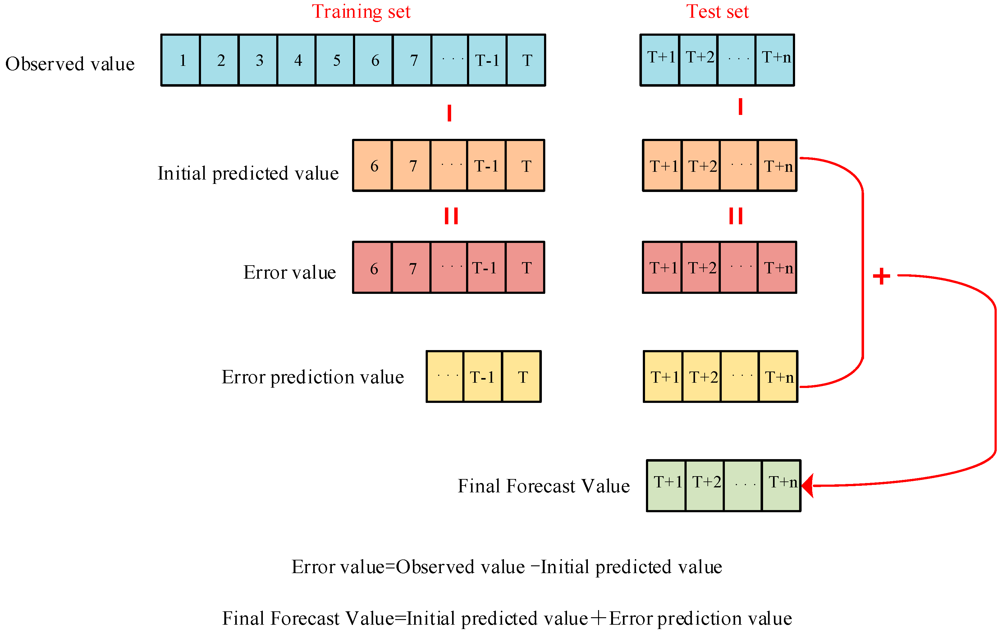
Figure 1. Flowchart of error correction process.
Water 16 02871 g001
Figure 2. A structural diagram of the TVFEMD-IJS-IFELM-OSELM water level prediction model.
Water 16 02871 g002
Figure 3. Decomposition components of Taihu’s daily water level time series.
Water 16 02871 g003
Figure 4. NSE for different models.
Water 16 02871 g004
Figure 5. Daily water level forecasts for Taihu in the 2016–2018 period.
Water 16 02871 g005
Figure 6. Comparison of forecast errors for different models.
Water 16 02871 g006
Figure 7. A 95% scatter plot for Taihu’s daily water level prediction results.
Water 16 02871 g007
Table 1. Evaluation indicators and their formulas.
Evaluation IndicatorsFormula
Root mean square error
(RMSE)
1 n i = 1 n ( y i y ^ i ) 2
Mean absolute error
(MAE)
1 n i = 1 n y i y ^ i
Mean absolute percentage
error
(MAPE)
1 n i = 1 n y i y ^ i y i × 100 %
Nash–Sutcliffe efficiency
(NSE)
1 i = 1 n ( y i ^ y i ) 2 i = 1 n ( y i y ¯ ) 2
Table 2. Summary of forecasting results for different models.
ModelRMSEMAENSEMAPE (%)
ELM0.0357050.0168630.98580.4931
BP0.0377930.0181750.98620.4665
LSTM0.0300960.0177410.99120.4998
IFELM0.0245790.0151470.99410.4301
TVFEMD-IFELM0.0123590.0042620.99850.1084
TVFEMD-IFELM-OSELM0.0104740.0041950.99890.1101
TVFEMD-IJS-IFELM-OSELM0.0055620.0029950.99970.0824
Table 3. Peak water level predictions and errors for each model.
Year201620172018Average Error (%)
ModelMeasured Peak
Water Level (cm)
4.8603.6003.700
ELMPredicted Value (cm)4.5923.5893.6852.075
Predicted Absolute Error (%)5.5140.3060.405
BPPredicted Value (cm)4.6313.5953.6811.803
Predicted Absolute Error (%)4.7720.1390.514
LSTMPredicted Value(cm)4.7433.5853.7040.997
Predicted Absolute Error (%)2.4070.4170.108
IFELMPredicted Value (cm)4.7753.5883.6910.775
Predicted Absolute Error (%)1.7490.3330.243
TFVEMD-IFELMPredicted Value (cm)4.7843.5893.6980.641
Predicted Absolute Error (%)1.5640.3060.054
TFVEMD-IFELM
-OSELM
Predicted Value (cm)4.7963.5963.6960.512
Predicted Absolute Error (%)1.3170.1110.108
TFVEMD-IJS
-IFELM-OSELM
Predicted Value (cm)4.9013.6033.6990.316
Predicted Absolute Error (%)0.8370.0840.027
Disclaimer/Publisher’s Note: The statements, opinions and data contained in all publications are solely those of the individual author(s) and contributor(s) and not of MDPI and/or the editor(s). MDPI and/or the editor(s) disclaim responsibility for any injury to people or property resulting from any ideas, methods, instructions or products referred to in the content.