The Effect of Different Swell and Wind-Sea Proportions on the Transformation of Bimodal Spectral Waves over Slopes

Abstract

In the laboratory experiment, 1:25 scaled models are constructed to investigate the effect of different swell and wind-sea proportions on the wave transformation. The source of the wave spectrum is related to the wave conditions in the Gulf of Guinea. Swell from the westerlies and local wind-sea forms the bimodal spectral waves in the region. To better understand the transformation of bimodal spectral waves, a series of wave conditions are measured by the wave gauges in a wave flume. Based on the wave spectrum at the Bight of Benin, the wave transformation along the slopes and variations of different swell proportions are analyzed. The result of the wave height variations shows that the slope and swell proportion play a significant role in the maximum wave height, and the wave height has an upward trend with a large swell proportion. The analysis of wave nonlinearity is conducted, showing that the large swell proportion in the wave spectrum leads to a more significant nonlinearity before wave breaking. Combining the variations of wave height and wave nonlinearity, the influence of bimodal spectral waves on nearshore wave prediction, shoreline change, marine operations, and structure design is discussed.

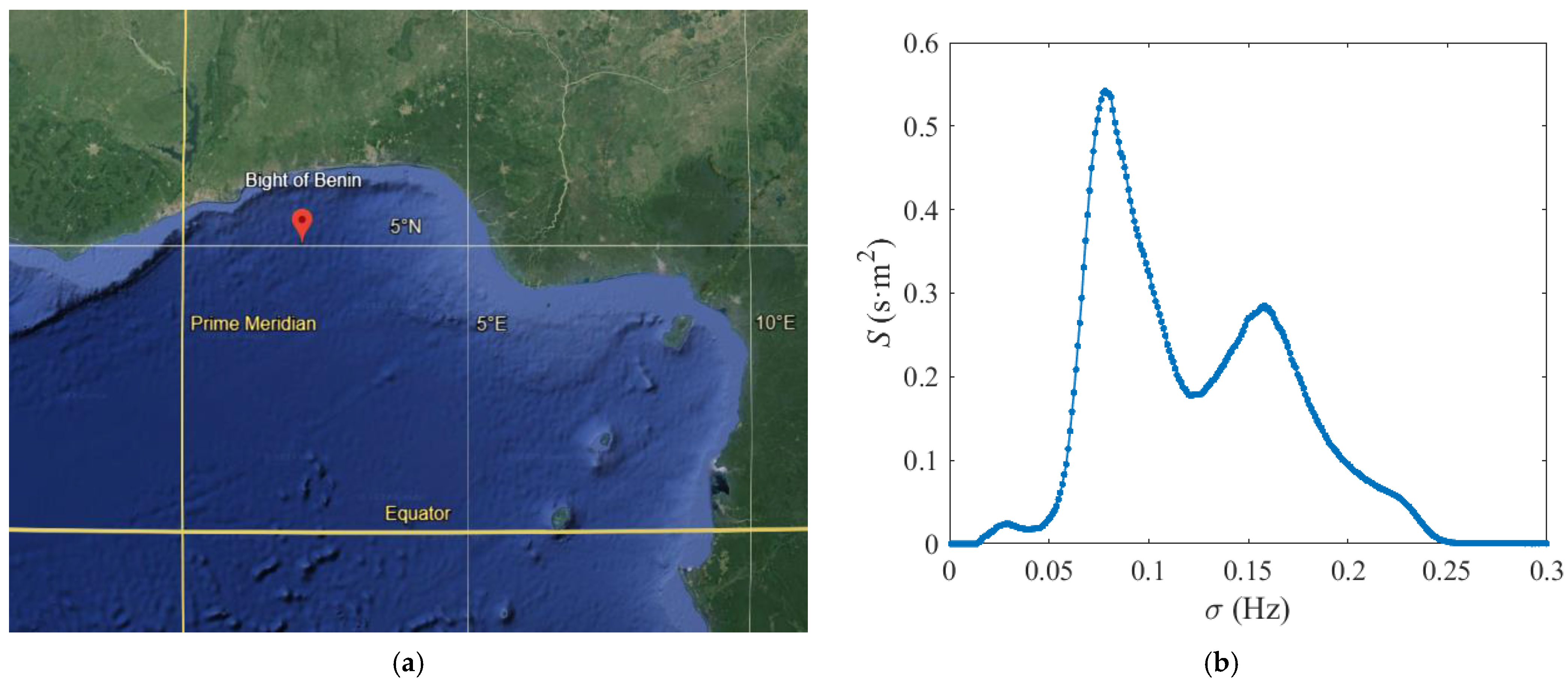
1. Introduction

The Gulf of Guinea is located in the eastern tropical Atlantic, around Africa. It is an open sea exposed to multiple wind wave systems. Two of these systems are the main components of local waves. They are the local short waves in the tropical band and the long wave system from the strong westerlies in the South Atlantic [1]. In the local wave system, the short wave generated by the wind is called wind-sea. Far from the Gulf of Guinea, wind waves generated in the strong westerlies travel for a long distance, and the wavelength becomes larger in the propagation. This long wave is called a swell. There is a clear distinction between these two types of wind waves in terms of the average wave period. The coexistence of wind, sea, and swell results in the complex wave condition in this area.

In order to study the complex wave conditions and the physical characteristics of waves, the wave spectrum is a fundamental tool. The wave spectrum can describe the distribution of wave energy at different frequencies and directions [2]. With this tool, some properties of ocean waves can be calculated. Bimodal spectral waves are a type of ocean wave that is characterized by the presence of two distinct peaks in the frequency spectrum. As the condition in the Gulf of Guinea is, the wave spectrum there represents the combination of two distinct wave systems: wind-sea and swell. The two wave systems can interact and modify one another [3]. Indeed, the properties of swell and wind-sea are significantly different. Winds are generated by local winds that blow over the sea surface with short wavelengths and periods. These waves tend to be responsive to changes in wind speed and direction [4]. On the other hand, swells often travel a long distance from their sources, generated by winds in remote regions of the ocean [5]. Compared to wind-sea, swell has a longer wavelength and wave period, and its wave duration is longer in deep water. Swell waves can propagate across entire ocean basins, carrying energy from thousands of kilometers away [6]. The different types of wave energy from the wind, sea, and swell have independent energy peaks in the wave spectrum. In a bimodal wave spectrum, wind waves occupy the high-frequency range and swells occupy the low-frequency range [7]. With respect to the unimodal wave spectra, the structure of wave groups is strongly modified in the bimodal condition [8]. The interaction among the components of the wind, sea, and swell has shown nonlinearity effects. These interactions are complex when the peaks of these two components become close to each other.

For laboratory experiments, many studies of the irregular wave transformation are performed. In previous research, the study of the wave spectrum has contributed to many practical applications. Because we are advancing our understanding of waves, wave spectra are extensively used in various applications related to ocean waves. Properties and parameterization of the wave spectrum are studied to explain some physical characteristics of waves in different ocean regions [9]. The variation in wave height or wave period may differ significantly depending on the coastal location. Wave characteristics in a particular region can have a profound impact on marine activities, coastal environments, and offshore structures [10]. The design of the offshore structures needs to consider the local wave characteristics. An analysis of the wave spectrum can be performed to derive the wave characteristics. This helps to estimate the wave force and ensure the offshore structures are durable enough to operate efficiently and safely. In predicting wave-induced forces on ships, the study of the bimodal spectrum can be used for vessel heading selection during the planning and execution of marine operations [11].

Another focus of research is wave transformation. In coastal areas, studies of wave transformation include wave shoaling and wave breaking. These phenomena involve various physical factors, such as the seafloor slope, wave amplitude, and water depth [12]. In intermediate-depth and shallow water, the effects of wave shoaling have crucial impacts on the wave transformation. The height of the waves changes before they break, and the shape of the waves deforms with interaction between the wave components. Therefore, the process of wave shoaling is significantly nonlinear. The behavior of the waves is not only proportional to the depth of the water but also depends on other factors, such as the wavelength and the slope of the seafloor [13]. Nonlinear interactions between waves cause the wave shape to distort from a simple sinusoidal pattern to more complex shapes [14]. For bimodal spectral waves, two kinds of different nonlinear interactions exist: swell and wind-sea, respectively. The study of the nonlinear wave transformation is important for accurate predictions of offshore wave characteristics. It has practical applications in coastal engineering projects such as breakwaters in coastal areas, and prediction of tropical cyclone waves [15,16].

Current research on bimodal waves studies their relevance to the theoretical wave spectrum. The actual bimodal spectrum can be estimated by independent components of swell and wind-sea [17]. The JONSWAP spectrum model is often used as an approximate estimation for the wind-sea part. The wave height in a bimodal wave condition has a relationship with both the swell and wind-sea parts. Based on the reconstructed bimodal wave spectra, the relationship seems to be linear between the overall wave height and the independent significant wave height of one part [18]. In this study, the main content focuses on the characteristics of bimodal spectral waves located in the Gulf of Guinea. To describe the formation of waves, the wave spectra are produced from measured wave data in the local sea area of the Bight of Benin on the Western African coast. To study the interaction between the wind, sea, and swell in the bimodal wave spectra, the wind, sea, and swell proportions are used as variables. A comparative analysis of unimodal and bimodal wave spectra is conducted. This physical modeling experiment is a generalized study of the local wave conditions. It provides fundamental information about the bimodal spectral wave in Benin and may contribute to coastal construction.

The rest of this article is organized as follows: Section 2 describes the wave flume, physical instruments, and wave conditions. Section 3 presents the data on water surface elevations, the analysis of wave height distribution, and the effect of swell proportions. This section then states the variation in wave nonlinearity and discusses the influence of bimodal spectral waves. Section 4 discusses the considerations of the study regarding engineering applications and gives a short conclusion.

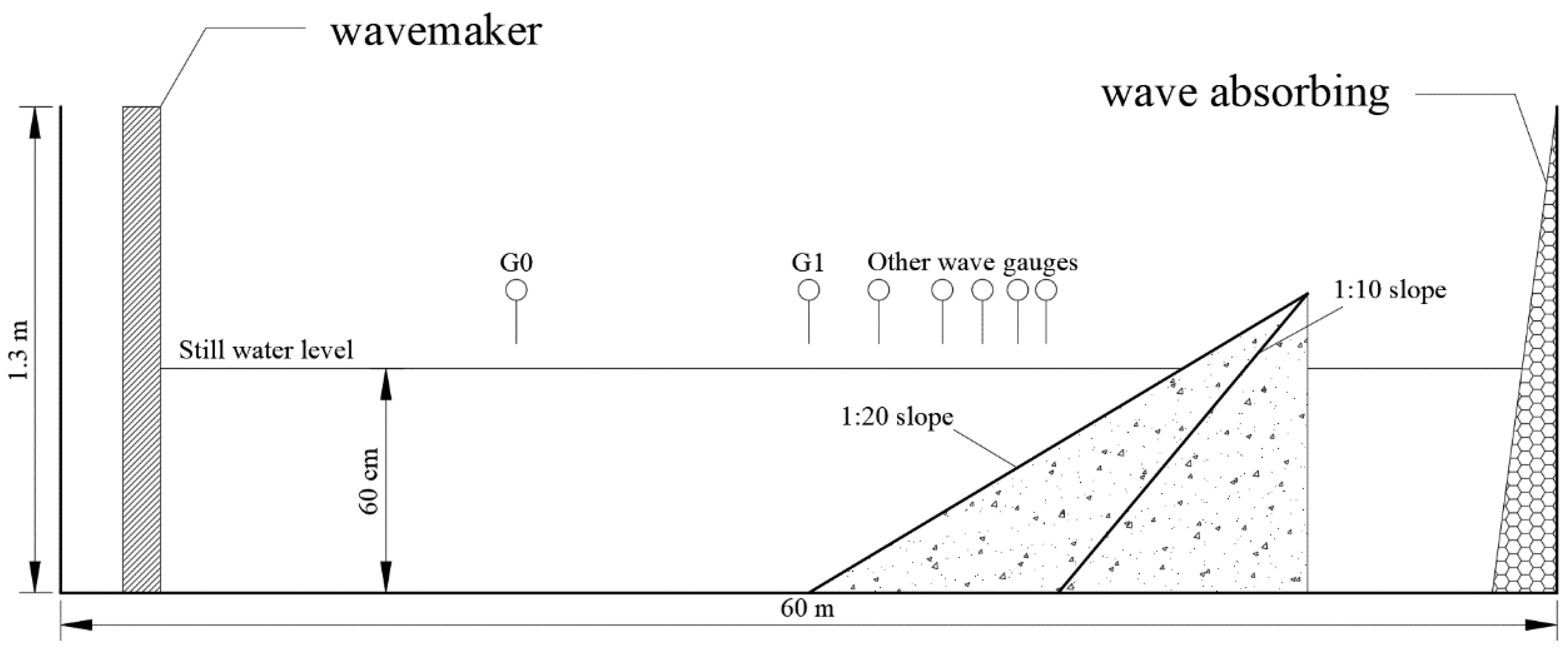
2. Experimental Setup

2.1. Wave Flume and Instrumentation Setup

The experiment is conducted in the Harbour and Waterway Engineering and Coastal Marine Science Experimental Center at Hohai University. The physical model is set in the wave flume in the marine engineering laboratory. The length of the wave flume is 60 m, the inner width is 1 m, and the inner height is 1.3 m. The two ends of the wave flume are respectively equipped with a wavemaker of piston type and a wave-absorbing system, as shown in Figure 1. The wavemaker can generate regular waves and irregular waves. The wave spectra of the irregular waves can be customized according to the input parameters of the spectra. The system can calculate the reflected waves to reduce the impact on the aimed wave spectra. The slope models are set in the wave flume near the wave-absorbing system.

The selection of slope is based on the typical beach profile of Benin (a country in West Africa). The beach in Benin has an annual variation in slope and coastline [19]. In this research, straight slope models are used to simplify the nearshore slope condition for a generalized study. In the experiment, both the 1:10 slope model and the 1:20 slope model were tested. The geometric scale of the slope models is 1:25. The bottom of the slope model is filled with sand and gravel, and the surface is treated with cement plaster. The still water level in the wave flume in the experiment is 60 cm before wave generation.

Water surface elevations are sampled by capacitance-type wave gauges. Figure 1 shows the locations of the wave gauges. The sampling frequency of the wave gauges is 100 Hz, and the time interval of elevation data is 0.01 s. The elevation data are sampled after the wave arrives at the slope and a stable wave system form. The sampling duration of the water surface elevations lasts from t = 0 s to t = 400 s, including more than 200 irregular wave cycles. The first wave gauge, G1, is located at the toe slope. The specific distribution positions of each wave gauge are presented in

Table 1. Positions of wave gauges in different tests.

Slope	Wave Gauges	Distance from G1 X (m)	Water Depth h (cm)
1:10	G1	0.0	60
	G2	1.0	50
	G3	2.0	40
	G4	2.5	35
	G5	3.0	30
	G6	3.5	25
	G7	4.0	20
	G8	4.3	17
	G9	4.6	14
1:20	G1	0.0	60
	G2	2.0	50
	G3	4.0	40
	G4	5.0	35
	G5	6.0	30
	G6	7.0	25
	G7	8.0	20
	G8	8.5	17.5
	G9	9.0	15
	G10	9.5	12.5

. In addition, the wave gauge G0 is located in front of the wave gauge G1 in an appropriate position. In tests, the wave gauge G0 is used to verify the wave properties between the incident wave spectrum and the theoretical wave spectrum. Therefore, the input parameters of the wavemaker could be adjusted in the test.

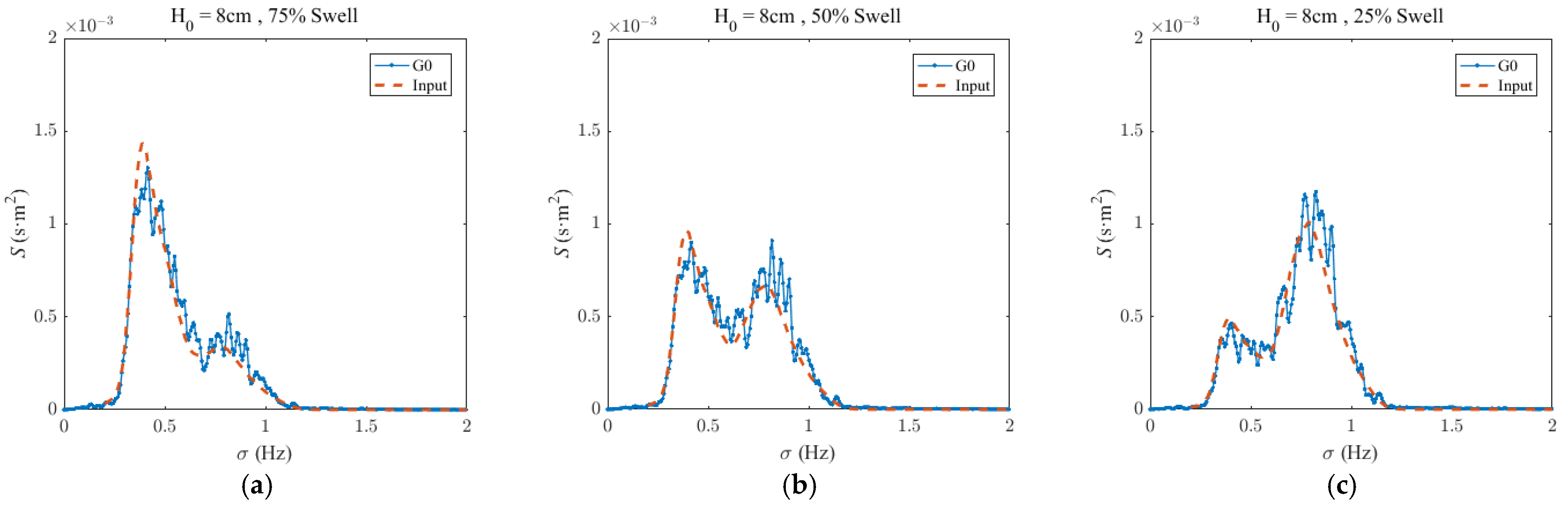
2.2. Wave Conditions

The Bight of Benin is located in the Gulf of Guinea, as shown in Figure 2a. This area is affected by the long-period swell waves propagating from near 45° to 60° south latitudes in the Atlantic Ocean [1]. Together with the short-period local wind, the wave spectrum forms a typical bimodal spectrum. Figure 2b shows an average wave spectrum measured in deep water. The wave data are measured from 19 December 2020 to 12 January 2021. It represents the typical wave conditions at the Bight of Benin in the summer of the Southern Hemisphere. In most cases, the range of the significant wave height is between 0.75 m and 1.75 m, and the range of the peak period of wave spectra is between 8 s and 16 s. Among all the wave conditions, the maximum significant wave height could reach 3.1 m, and the maximum peak of the wave spectrum is 22 s. The data are based on the wave simulation from 1981 to 2006. In the experiment, the geometric scale of the physical model is 1:25 and the time scale is 1:5. The models follow the Froude similarity law, given the predominant gravity waves. The test refers to the range of local wave heights in the Gulf of Guinea. Combining the 1:25 scale, three kinds of significant wave heights are set up in the experiment. It is the target significant wave height of the incident wave spectrum. In actual tests, the wave height of irregular waves is controlled around the target height.

The input parameters of the wavemaker are adjusted according to the wave spectrum in Figure 2b. In the local measurement, the swell peak frequency is about 0.8 Hz, and the wind-sea peak frequency is about 1.6 Hz. The dividing of swell and wind-sea is based on the JONSWAP Spectrum [20]. The two spectra with the same peak frequencies are used to represent different parts of wind, sea, and swell in the bimodal wave spectrum. Therefore, the peak frequency parameter stays constant. The other parameters are changed in order to ensure that the superposition of the two spectra fits the original spectrum as well as possible. As a result, the fundamental spectra of the swell part and the wind-sea part are determined. By adjusting the energy proportion of the swell part and wind-sea part in the total wave energy of the incident wave spectrum, five kinds of incident wave spectra are set up in the experiment. A 25% change in swell proportion is used as a stage. The unimodal wave spectra of swell and wind-sea are also included as comparisons. Combining the conditions of different wave heights and wave spectra, the detailed cases of the experiment are listed in

Table 2. Input conditions for the wave spectrum.

Wave Spectrum	Case	Significant Wave Height H0 (cm)	Swell Proportion	Wind-Sea Proportion
Unimodal	1	12	100%	0%
	2	8	100%	0%
	3	4	100%	0%
Bimodal	4	12	75%	25%
	5	8	75%	25%
	6	4	75%	25%
	7	12	50%	50%
	8	8	50%	50%
	9	4	50%	50%
	10	12	25%	75%
	11	8	25%	75%
	12	4	25%	75%
Unimodal	13	12	0%	100%
	14	8	0%	100%
	15	4	0%	100%

.

The verification of the incident wave condition is performed by the wave gauge G0. As shown in Figure 1, it is located in the middle of the wavemaker and the wave gauge G1. In the pilot tests, the wave spectrum at the wave gauge G0 is compared to the theoretical wave spectrum in terms of the energy proportion of swell, peak frequency, and significant wave height of the theoretical wave spectrum. There are some deviations between the input parameters of the wavemaker and the actual wave-making results. To improve the accuracy of the wavemaker, adjustments to the input parameters are performed in the pilot tests. Figure 3 illustrates the comparison of the wave spectra measured at the wave gauge G0 and the theoretical wave spectrum in some cases.

3. Experimental Results

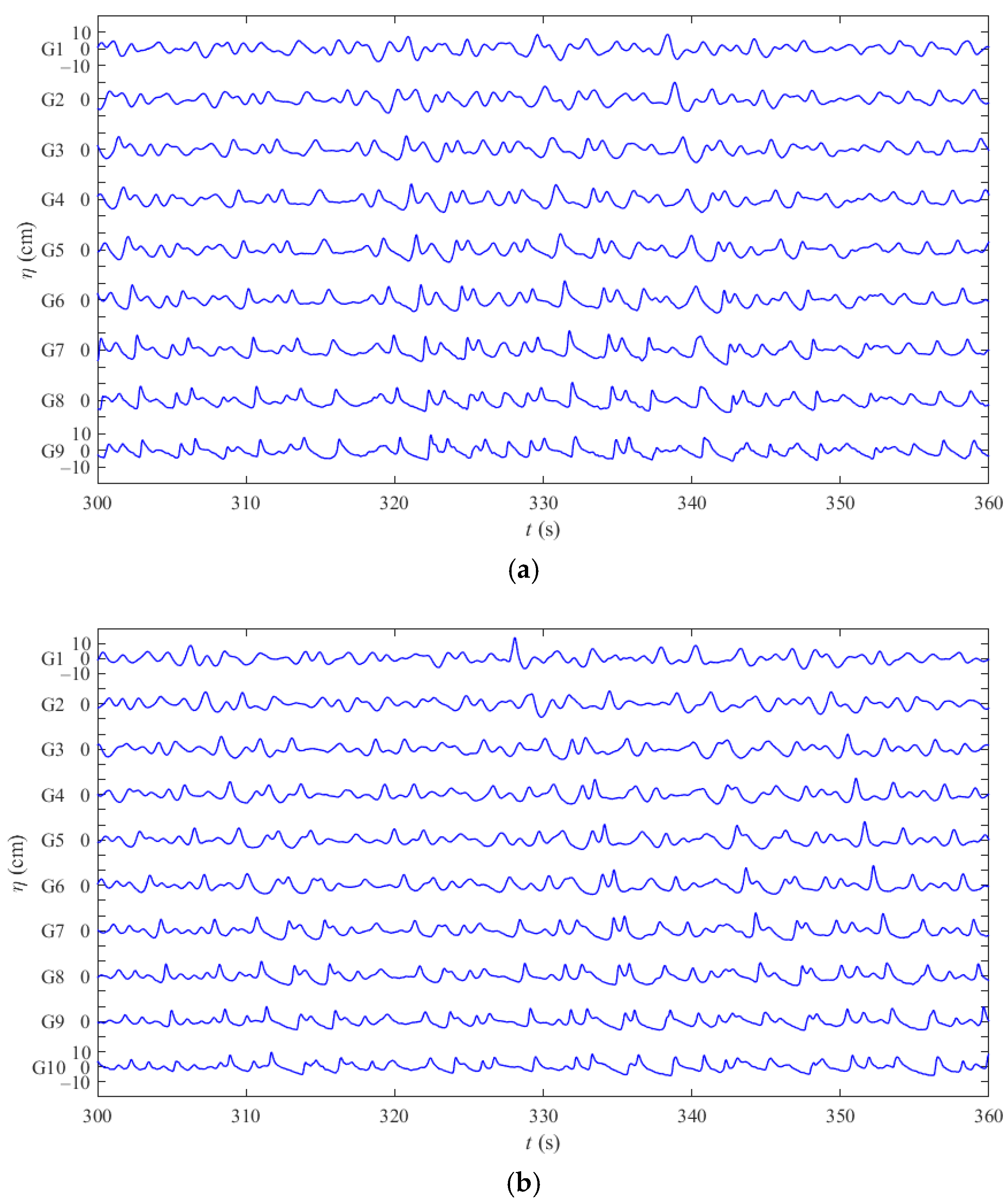
3.1. Variation in Water Surface Elevations

Taking case 7 as an example, the measurements of the water surface elevations by wave gauges are shown in Figure 4. In these figures, the red arrow lines show the effect of wave shoaling on transformation. When the irregular waves first reach the toe slope, the waves still maintain an approximate shape of linear waves. As waves propagate over the slope, the crest of the wave becomes sharper, and the trough of the wave is elongated. At the same time, some waves have an increase in wave height before breaking. This wave shoaling process is mainly presented between the wave gauges G0 and G7. In locations with the last 2 or 3 wave gauges, some waves with a large wave height are breaking. In these cases of 12 cm incident wave height, many waves have reached the water depth limitation of breaking. It causes a decrease in the significant wave height in shallow water. In these tests, the type of breaking water waves is between spilling and plunging. For the bimodal spectral waves, swells with longer wavelengths tend to be plunging waves, and wind-seas with shorter wavelengths tend to be spilling waves.

During a wave period, the symmetry of some waves decreases significantly. For example, measured by the wave gauge G1, the wave crests at about 329 s, 338 s (Figure 4a), and 306 s, 340 s (Figure 4b) are symmetrical in front and back. Then the crests of these waves gradually shift from the middle of adjacent troughs. During propagation, wave crests shift in a forward direction. For irregular waves with small wave heights, the front surface of waves is gradually becoming steeper than the back surface.

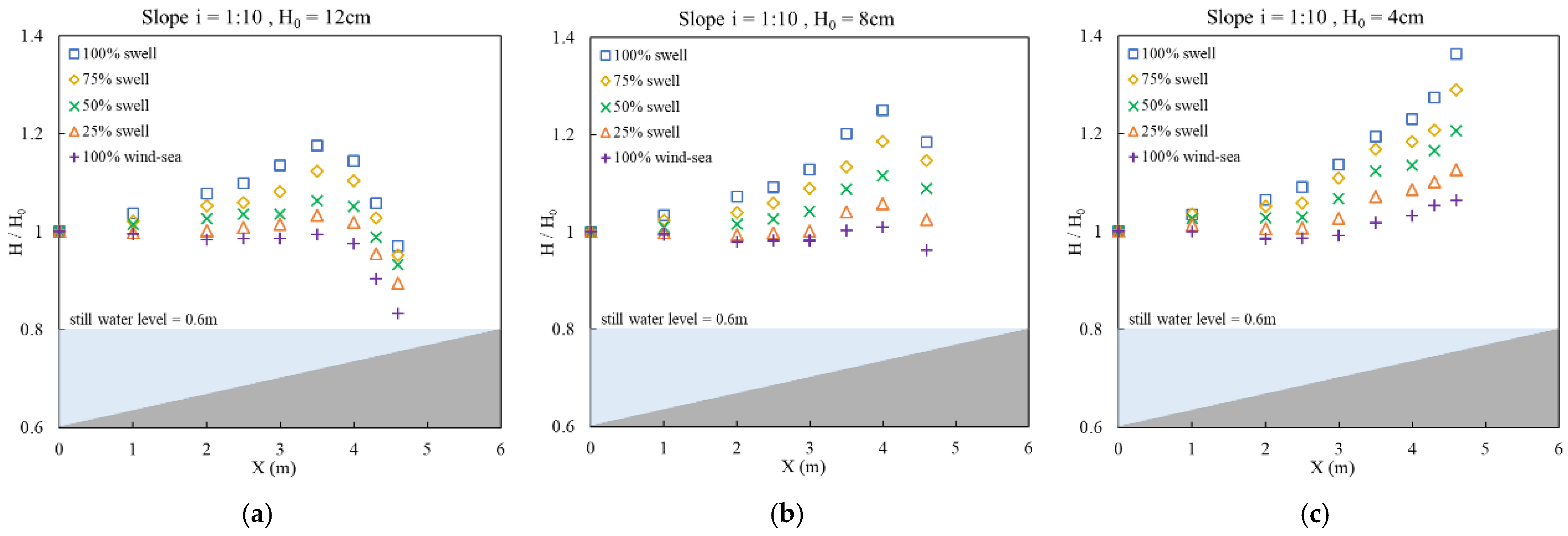
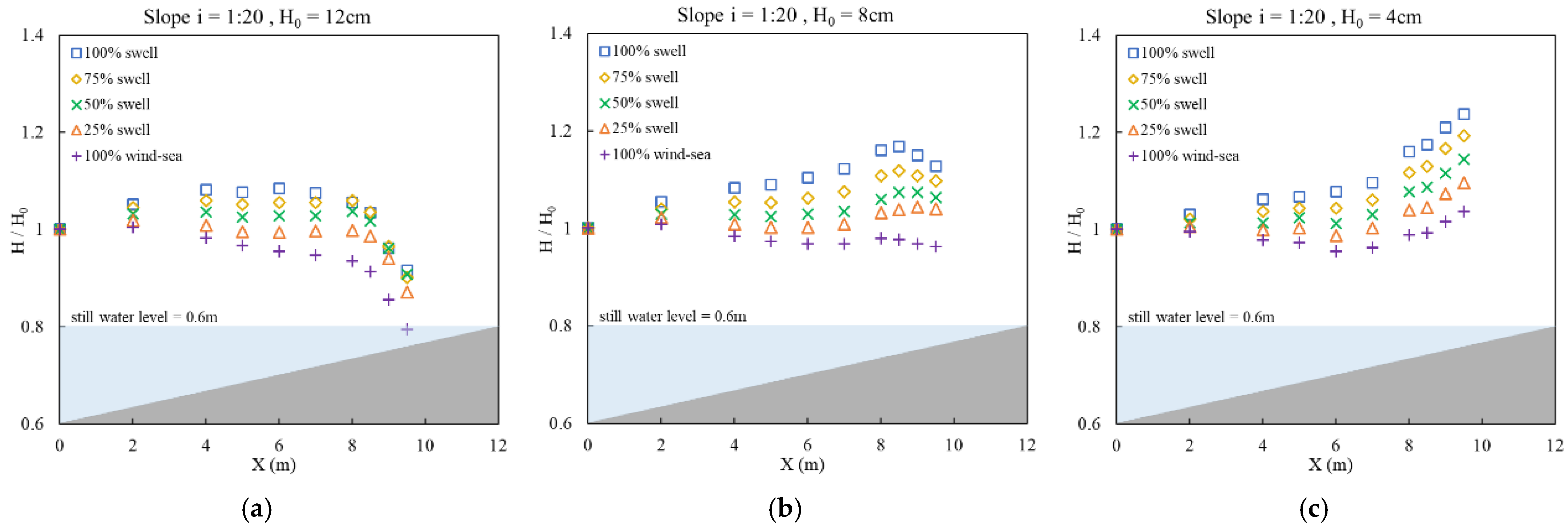
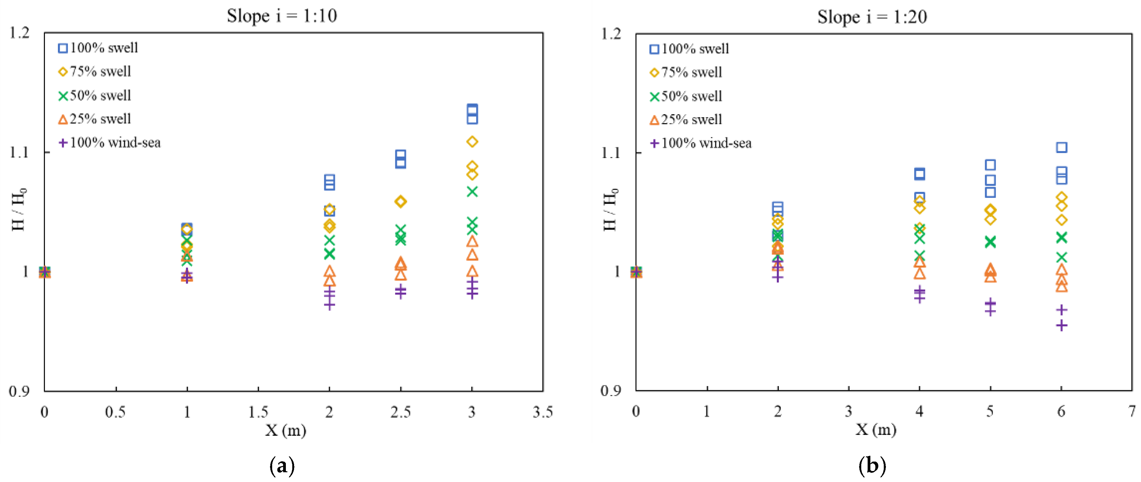
3.2. Wave Height Distribution on Slopes

Wave gauge measurements are used to calculate significant wave heights along the slope. The result of the 1:10 slope test is shown in Figure 5, and that of the 1:20 slope test is shown in Figure 6. For the comparison of cases, significant wave heights are displayed in ratios to those at wave gauge G1.

In these figures, it can be seen that the maximum significant wave height occurs in 100% swell cases. For example, in 12 cm wave height cases (Figure 5a), the maximum wave height ratio is 117.5% at wave gauge G6. For the unimodal wave spectrum of wind-sea, the wave height ratio is 99.4% at the same location. In the bimodal wave spectrum, as the swell proportion rises to 50%, the wave height ratio also rises to 106.3%. In the wave transformation on the slope, the swell proportion in the bimodal wave spectrum can influence the maximum significant wave height. When the swell proportion increases, the maximum height also increases. Compared to the 1:20 slope test (Figure 6), as the slope decreases, the maximum significant wave height of the swell decreases. In the 100% swell cases, maximum ratios are listed as follows:

• 1:10 slope: 117.5% (12 cm), 125.0% (8 cm), 136.2% (4 cm);
• 1:20 slope: 108.4% (12 cm), 116.8% (8 cm), 123.8% (4 cm).

For wind-sea, the slope does not have a significant effect. To summarize, for bimodal spectral waves, there are two main factors that can influence the maximum wave height. One is the swell proportion, and the relationship is approximately linear. When the swell proportion becomes larger in the wave spectrum, the wave height becomes larger and is closer to the 100% swell condition. The slope influences the wave height, mainly on the swell part. A steeper slope in shallow water results in a larger swell wave height.

Before wave breaking, wave heights along the slope also change due to wave shoaling. Figure 7 presents the variation in significant wave height when the water depth is greater than 30 cm. This includes all the cases of one slope test. In this water depth, irregular waves do not reach the water depth limitation of breaking. It can be seen that, in cases of the same swell proportion, the variation in significant wave height is similar. In the intermediate water depth, for unimodal spectral wind-seas, wave height decreases slightly with decreasing water depth. However, the bimodal spectral wave height may increase according to the swell proportion. When the swell proportion increases, the wave height tends to increase. Meanwhile, as the slope is steeper, the swell wave height also tends to increase. Since the water depth limitation for breaking is not reached, incident wave heights have no effect on the process of wave shoaling. In summary, the swell proportion in a bimodal wave spectrum can affect the wave height trend. Wind-sea wave heights tend to decrease slightly, while swell wave heights tend to increase. The wave-shoaling effects of swell and wind-sea are different in the intermediate water depth.

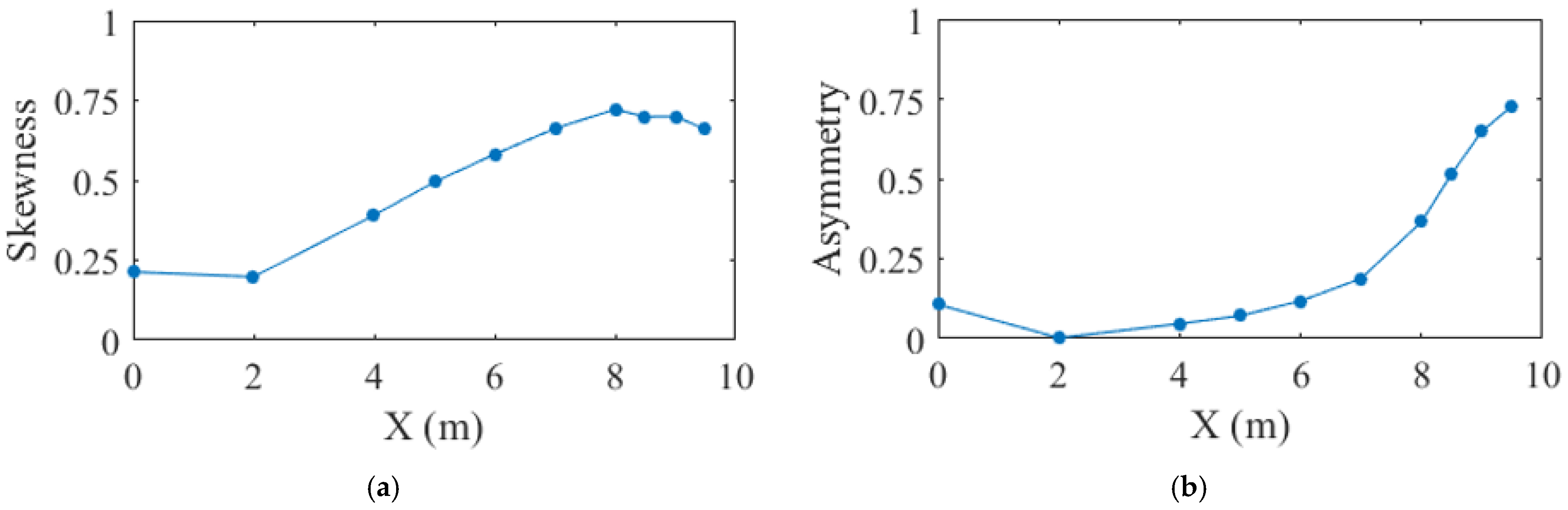
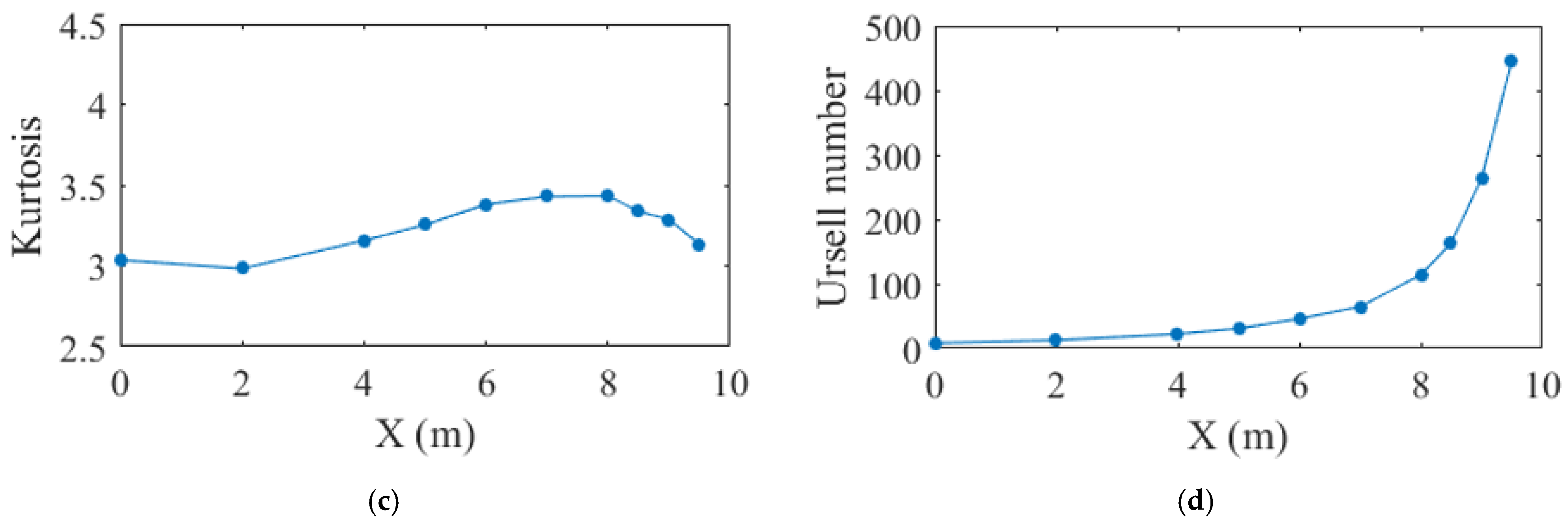
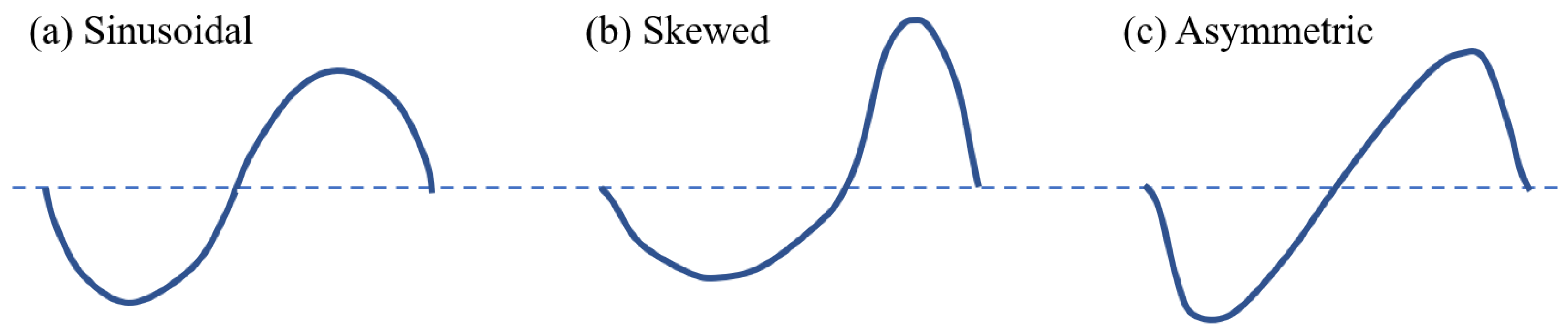
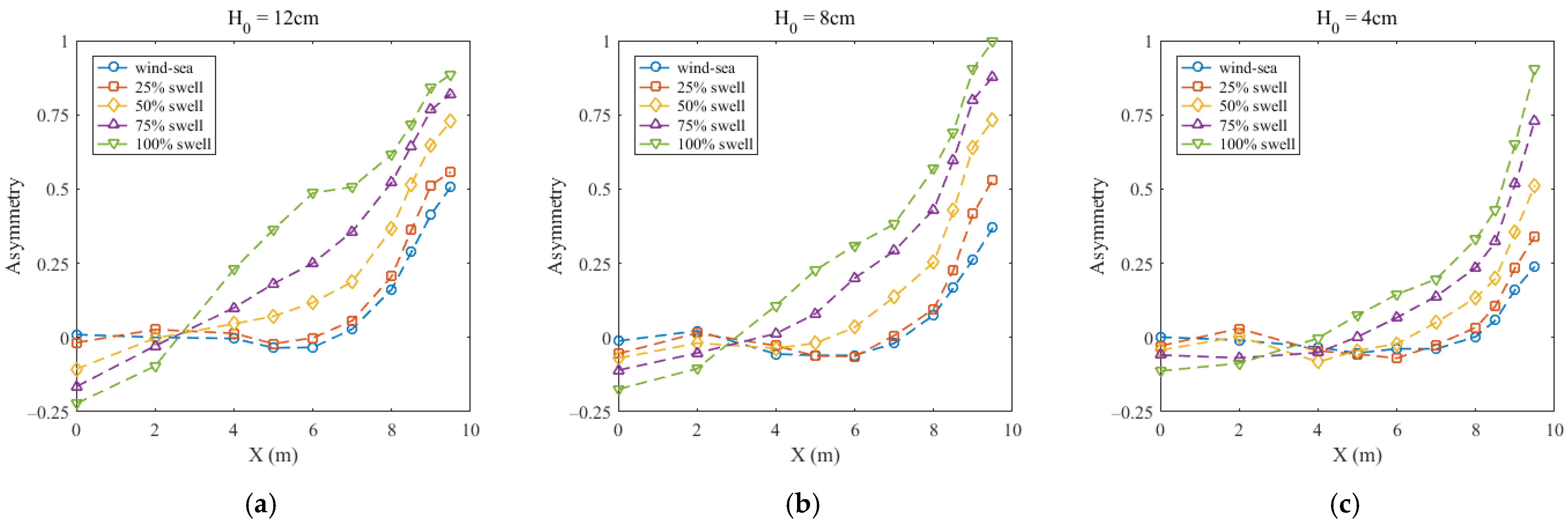
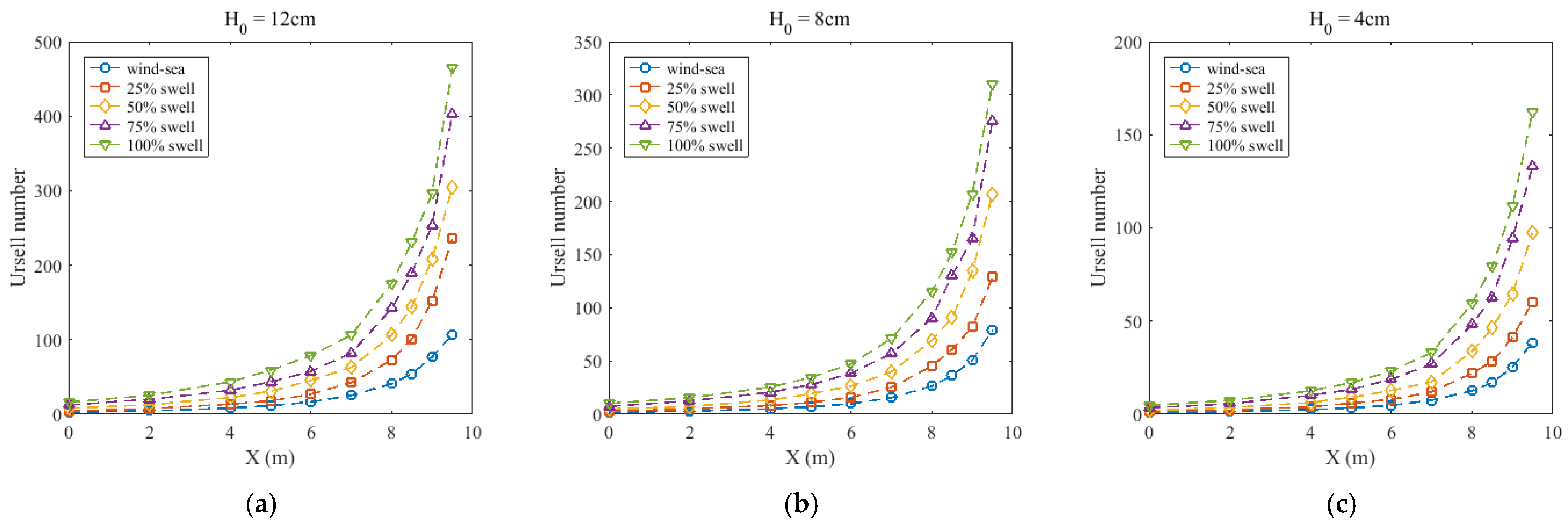
3.3. Nonlinear Indicators of Waves

The nonlinearity of waves refers to their deviations from a sinusoidal shape. When waves encounter a shallow water depth, wave nonlinearity occurs with changes in wavelength and wave height. The following four indicators are used to describe the wave nonlinearity:

Skewness refers to the asymmetry of a probability density function that deviates from a normal distribution. The skewness S is defined as:

$$S(\eta )=\frac{k_3}{k_2^{3/2}}$$

(1)

where η is the water surface elevation, $k_2$ is the second central moment of η, and $k_3$ is the third central moment of η.

Asymmetry describes the leaning forward or backward of the wave relative to the crest. The asymmetry A is defined as:

$$A\left(\eta \right)=S\left(H\right(\eta \left)\right)$$

(2)

where H is the Hilbert transform.

Kurtosis refers to the flatness or steepness of a probability density function that deviates from a normal distribution. The kurtosis K is defined as:

$$K(\eta )=\frac{k_4}{k_2^2}$$

(3)

where $k_4$ is the fourth central moment of η.

The Ursell number describes the nonlinearity of long surface gravity waves on a fluid layer. The Ursell number U_r is defined as:

$$U_r=\frac{H{L}^2}{h^3}$$

(4)

where H is the significant wave height, L is the significant wavelength, and h is the mean water depth.

Taking case 8 as an example, Figure 8 presents the variation of four nonlinear indicators. In this case, wave propagation causes increase in the indicator values. The distribution of water surface elevations deviates from a normal distribution, and the wave shape deviates from a sinusoidal shape. Kurtosis describes the distribution of water surface elevations. K is 3 in a normal distribution. When the kurtosis becomes larger, the curve of a probability density function becomes a higher peak around the mean. For incident waves at wave gauge G1 (Figure 8c), K is close to 3. Then K has an increase in the wave shoaling process and a decrease after wave breaking. For water surface elevations, the increase in K means that the duration of the wave crest and trough becomes shorter. Skewness and asymmetry describe the wave shape. Linear waves have a sinusoidal shape (Figure 9a), in which S is 0 and A is 0. In Figure 8a,b, S and A both have an increase along the slope. For wave shapes, when S becomes larger, the wave crest is shorter and higher, and the wave trough is flatter and longer (Figure 9b). Meanwhile, when A becomes larger, the front face of the wave crest is steeper, and the rear face is gentler (Figure 9c). For water surface elevations, the variation in wave shape is also shown in Figure 4. These waves become more asymmetric along the horizontal axis and the vertical axis, marked by red arrow lines. As the Ursell number becomes larger, the wave nonlinearity increases, and the linear wave theory is no longer applicable.

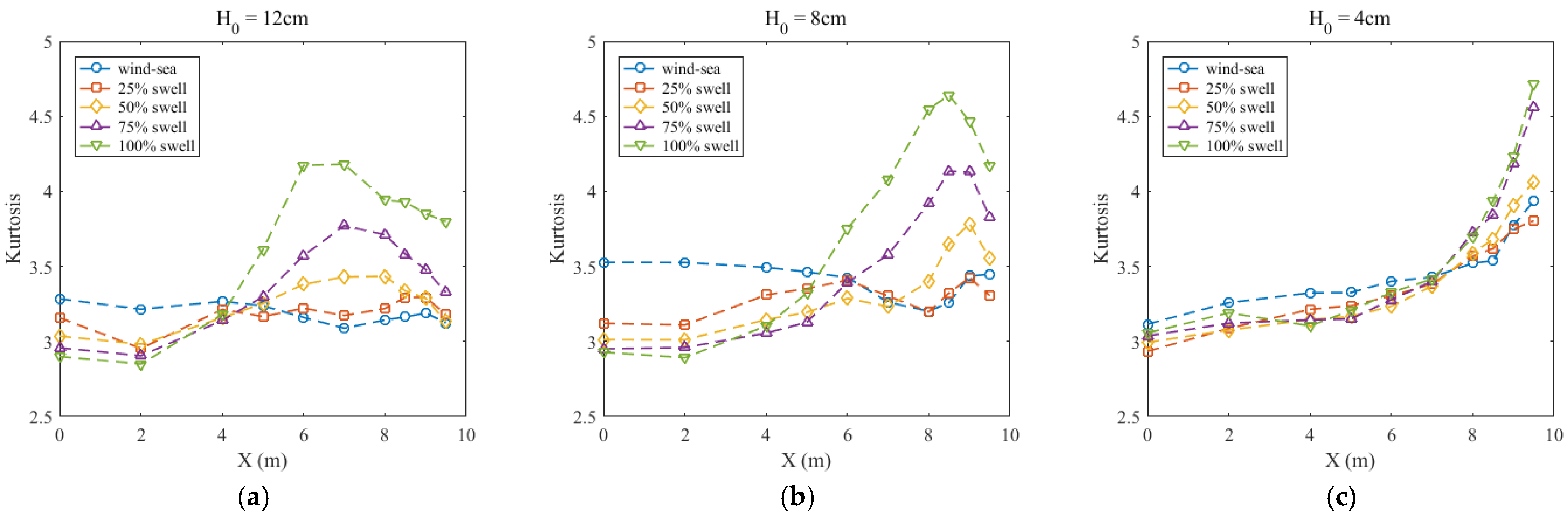
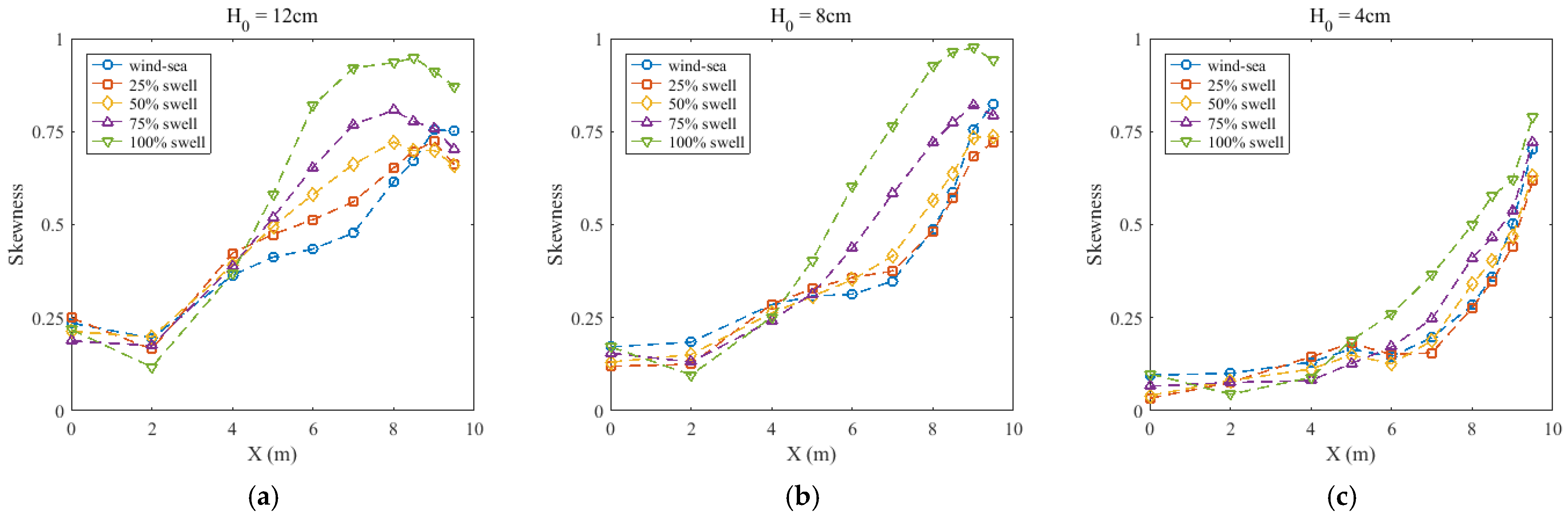
3.4. Variation in Wave Nonlinearity over Slopes

Taking the test of 1:20 slope as an example, Figure 10 presents the variation in kurtosis with different swell proportions. It is noticed that the maximum value of kurtosis appears in the 100% swell case of the same significant wave height. Meanwhile, the maximum value usually occurs before the wave breaks. The maximum values are 4.180, 4.641, and 4.712 for swell in cases of 12 cm, 8 cm, and 4 cm wave height. It means that smaller, more significant wave heights can result in a larger maximum kurtosis. According to the definition, swell has a shorter duration of wave crest and trough before wave breaking. In bimodal conditions, 75% of swell proportion cases show high similarity to the variation in swell. Their kurtosis also peaks before the wave breaks and becomes larger when the wave height decreases.

The variation in wave skewness is presented in Figure 11. Along the 1:20 slope, wave skewness has a common increase. It can be noticed that the skewness increase in swell is larger than wind-sea in a specific water depth from the wave gauge G3 to G6. In this 2.5 m interval on the 1:20 slope, 75% of the swell proportion cases have a significant increase, and 25% of the swell proportion cases are similar to the wind-sea. The increase in skewness is explained by the Stokes wave. For the bimodal wave spectrum, the peak frequency shifts from high to low as the swell proportion increases. Lower peak frequencies result in a longer mean wave period in irregular waves. Because of the same still water level in tests, incident wavelengths of a larger swell proportion are longer. The Stokes wave suggests that the asymmetry between the wave crest and trough will intensify as the ratio of water depth to wavelength becomes smaller. Therefore, this nonlinear correlation causes a larger skewness increase in swell in the specific water depth. Another difference is the influence of wave breaking. In cases of 12 cm and 8 cm of significant wave height, wave breaking occurs in the shallow water. The skewness of the wind-sea does not appear to decrease, while the swell does after wave breaking. For a bimodal wave spectrum, this decrease appears when the swell proportion is about more than 50%.

Figure 12 shows the wave asymmetry of different significant wave heights along the slope. In this section, asymmetry is taken in negative values. When waves propagate on the flat seabed, the wind-sea asymmetry is close to 0, while the swell asymmetry is not. It indicates the slight leaning backward of the swell in the deep water. But on the slope, there is a increase in the swell asymmetry in the intermediate water depth. This nonlinear variation process of swell is mainly from X = 2 m to X = 6.5 m. Meanwhile, the wind-sea asymmetry still fluctuates around 0. The swell has a more significant trend of leaning forward. As the swell proportion decreases from 75% to 25% in the bimodal wave spectrum, the asymmetry transitions from swell to wind-sea. Combined with the increase in skewness, the swell has a more significant nonlinear change in this water depth. It can be seen that swell has a larger maximum value of asymmetry than wind-sea. In cases of the same wave height, as the swell proportion increases, bimodal spectral waves will have a larger maximum asymmetry. The asymmetry of significant waves is closely related to the subsequent wave-breaking phenomenon. In this 1:20 slope test, when wave breaking occurs, waves with large asymmetry tend to be plunging waves.

The Ursell number describes wave nonlinearity in general, as shown in Figure 13. As the Ursell number increases, the wave asymmetry along the horizontal axis and the vertical axis increases. To summarize, water depth and swell proportion are the two main factors. For bimodal spectral waves, the wave nonlinearity is more significant at large swell proportions and in shallow water. The changes in kurtosis, skewness, and asymmetry comprehensively indicate the increase in wave nonlinearity. For these indicators, the linear variation in the swell proportion does not result in a linear distribution. Especially in shallow water, the wave nonlinearity of bimodal spectra is not appropriate to be estimated by unimodal spectra. The swelling proportion of the bimodal spectrum mainly influences the trend of nonlinear change in shallow water. When the swell proportion is large, the trend is similar to the unimodal swell generally. Otherwise, the trend is similar to the unimodal wind-sea. The 50% swell proportion case is somewhere in between and cannot be seen as a linear average of swell and wind-sea.

4. Discussion and Conclusions

To investigate the transformation of bimodal spectral waves, a 1:25 scaled physical experiment has been conducted in the wave flume. In the series of experimental tests, the incident wave spectrum is the main control condition. The original wave spectrum is an average spectrum measured in the local summer of the Southern Hemisphere. The JONSWAP spectra are used to fit the two peaks. Swell and wind-sea are both considered in different tests. The design of this physical model is based on field measurements at the Bight of Benin, in the Gulf of Guinea. The slopes are simplified models of the nearshore slope condition on the Benin coast, covering two usual conditions during coastal evolution. The study of the range of wave heights in the test focuses on the local waves. The wave heights correspond to the most common cases and a few larger values at the Bight of Benin.

The characteristics of the bimodal wave spectrum with different swell proportions are investigated. The following are the conclusions from this study:

• For bimodal spectral waves, two main factors influence the maximum wave height. One is the swell proportion, and the other is the slope. An increase in these two factors causes a higher maximum wave height. The swell proportion also influences the effect of wave shoaling. Swell has a larger increase in significant wave height. The relationship between different swell proportions in the bimodal spectrum and the unimodal spectrum is approximately linear in wave height.
• Wave nonlinearity is determined by the water depth and swell proportion. The water depth, wavelength, and wave height control the stages of nonlinear changes. The swelling proportion of the bimodal spectrum influences the trend of nonlinear change in shallow water. The kurtosis, skewness, and asymmetry of swells are larger than wind-sea. The trend of large swell proportions is similar to the unimodal swell. The relationship seems not to be linear.

For the maximum significant wave height, the swell proportion and the slope of the seabed can cause notable differences. As the swell proportion of bimodal spectral waves increases, the maximum wave height increases. On a steeper slope, the maximum wave height is larger. Meanwhile, swell proportion can also affect the wave height trend. In the intermediate water depth, wind-sea wave heights tend to decrease slightly while swell wave heights tend to increase. The wave shoaling effect causes differences in the variation in significant wave height for bimodal spectral waves.

In some practical applications, the conclusions are discussed. In ocean wave height forecasts, satellite radar altimeters are used to measure the significant wave height directly [21]. On this basis, the wind wave models are used to predict the wave height of the coastal zone. In propagating from deep to shallow water depth, wave heights have different proportions of swell and wind-sea. For areas with seasonal variations in the bimodal wave spectrum, the prediction of significant wave height needs to be corrected. The long-term data on the wave spectrum measured by the nearshore devices is useful. In addition, large waves are sometimes caused by swells generated by large storms. The swell proportion will increase in this condition, resulting in a larger and more significant wave height near shore. For the design of nearshore structures, the local bimodal wave spectrum should be considered in the design of wave height. Wave heights also play a crucial role in planning and executing marine operations. When the swell proportion is large, nearshore vessels may encounter more dangerous conditions.

The variation in wave nonlinearity is described by four indicators. For bimodal spectral waves, as the swell proportion increases, the Ursell number increases. This indicator generally describes the degree of wave nonlinearity. Compared to the wind-sea, the swell has a larger maximum value of kurtosis and asymmetry. Also, the swell has a faster increase in skewness and asymmetry before wave breaking. The difference in wave nonlinearity has an influence on wave-driven currents and wave breaking. The asymmetric currents result in changes in sediment transport, leading to altered erosion or deposition along the shoreline [22,23]. In the Gulf of Guinea, swell and wind-sea proportions have annual variations due to the seasons. These variations lead to differences in wave nonlinearity, especially in nearshore areas. The asymmetric current also changes with the seasonal variation in the wave spectrum. Therefore, the properties of the bimodal wave spectrum may help in the prediction of sediment transport and coastal erosion patterns. Wave nonlinearity affects the shape of wave breaking, which has an influence on the durability and safety of nearshore structures [24,25]. For the design of nearshore structures, the swell proportion of the local bimodal wave spectrum needs to be considered.

In general, these results may have significant implications for coastal planning in areas with bimodal wave-spectral sea conditions. For example, in the coastal areas of the Gulf of Guinea., Results indicate that wave height and wave nonlinearity are related to swell proportions. Limited to the experiment in a wave flume, the effect of wave directionality is not considered. In actual wave conditions, the swell and wind may propagate in different directions. This needs to be further discussed based on local measurements. The swell proportion of the bimodal wave spectrum usually changes with the seasons. Future work may further investigate the combined conditions of wave spectrum, wave height, and seasonal variation in improving local coastal construction.

References

- Almar, R.; Kestenare, E.; Reyns, J.; Jouanno, J.; Anthony, E.J.; Laibi, R.; Hemer, M.; Du Penhoat, Y.; Ranasinghe, R. Response of the Bight of Benin (Gulf of Guinea, West Africa) coastline to anthropogenic and natural forcing, Part1: Wave climate variability and impacts on the longshore sediment transport. Cont. Shelf Res. 2015, 110, 48–59. [Google Scholar] [CrossRef]
- Goda, Y. A Comparative Review on the Functional Forms of Directional Wave Spectrum. Coast. Eng. J. 1999, 41, 1–20. [Google Scholar] [CrossRef]
- Toffoli, A.; Onorato, M.; Monbaliu, J. Wave statistics in unimodal and bimodal seas from a second-order model. Eur. J. Mech.-B/Fluids 2006, 25, 649–661. [Google Scholar] [CrossRef]
- Hanson, J.L.; Phillips, O.M. Wind Sea Growth and Dissipation in the Open Ocean. J. Phys. Oceanogr. 1999, 29, 1633–1648. [Google Scholar] [CrossRef]
- Alford, M.H. Internal Swell Generation: The Spatial Distribution of Energy Flux from the Wind to Mixed Layer Near-Inertial Motions. J. Phys. Oceanogr. 2001, 31, 2359–2368. [Google Scholar] [CrossRef]
- Semedo, A.; Vettor, R.; Breivik, Ø.; Sterl, A.; Reistad, M.; Soares, C.G.; Lima, D. The wind sea and swell waves climate in the Nordic seas. Ocean Dyn. 2015, 65, 223–240. [Google Scholar] [CrossRef]
- Vettor, R.; Guedes Soares, C. A global view on bimodal wave spectra and crossing seas from ERA-interim. Ocean Eng. 2020, 210, 107439. [Google Scholar] [CrossRef]
- Arena, F.; Soares, C.G. Nonlinear High Wave Groups in Bimodal Sea States. J. Waterw. Port Coast. Ocean Eng. 2009, 135, 69–79. [Google Scholar] [CrossRef]
- Hasselmann, D.E.; Dunckel, M.; Ewing, J.A. Directional Wave Spectra Observed during JONSWAP 1973. J. Phys. Oceanogr. 1980, 10, 1264–1280. [Google Scholar] [CrossRef]
- Clauss, G.F. Dramas of the sea: Episodic waves and their impact on offshore structures. Appl. Ocean Res. 2002, 24, 147–161. [Google Scholar] [CrossRef]
- Guachamin-Acero, W.; Portilla-Yandún, J. A study on vessel fatigue damage as a criterion for heading selection by application of 2D actual bimodal and JONSWAP wave spectra. Ocean Eng. 2021, 226, 108822. [Google Scholar] [CrossRef]
- Liu, P.L.F.; Losada, I.J. Wave propagation modeling in coastal engineering. J. Hydraul. Res. 2002, 40, 229–240. [Google Scholar] [CrossRef]
- Barthélemy, E. Nonlinear Shallow Water Theories for Coastal Waves. Surv. Geophys. 2004, 25, 315–337. [Google Scholar] [CrossRef]
- Wu, G.X.; Taylor, R.E. The coupled finite element and boundary element analysis of nonlinear interactions between waves and bodies. Ocean Eng. 2003, 30, 387–400. [Google Scholar] [CrossRef]
- Hur, D.-S.; Kim, C.-H.; Yoon, J.-S. Numerical study on the interaction among a nonlinear wave, composite breakwater and sandy seabed. Coast. Eng. 2010, 57, 917–930. [Google Scholar] [CrossRef]
- Shi, J.; Feng, X.; Toumi, R.; Zhang, C.; Hodges, K.I.; Tao, A.; Zhang, W.; Zheng, J. Global increase in tropical cyclone ocean surface waves. Nat. Commun. 2024, 15, 174. [Google Scholar] [CrossRef] [PubMed]
- Garcia-Gabin, W. Wave bimodal spectrum based on swell and wind-sea components. IFAC-PapersOnLine 2015, 48, 223–228. [Google Scholar] [CrossRef]
- Liu, X.; Chen, W.; Sun, Z.; Cai, Z.; Hou, Y. Investigation on the reconstruction of wave bimodal spectrum in the lagoon near islands and reefs. Ocean Eng. 2022, 265, 112615. [Google Scholar] [CrossRef]
- Abessolo Ondoa, G.; Bonou, F.; Tomety, F.S.; Du Penhoat, Y.; Perret, C.; Degbe, C.G.E.; Almar, R. Beach Response to Wave Forcing from Event to Inter-Annual Time Scales at Grand Popo, Benin (Gulf of Guinea). Water 2017, 9, 447. [Google Scholar] [CrossRef]
- Hasselmann, K.; Barnett, T.P.; Bouws, E.; Carlson, H.; Cartwright, D.E.; Enke, K.; Ewing, J.; Gienapp, A.; Hasselmann, D.; Kruseman, P. Measurements of wind-wave growth and swell decay during the Joint North Sea Wave Project (JONSWAP). Ergaenzungsheft Zur Dtsch. Hydrogr. Z. Reihe A 1973, 12, 1–95. [Google Scholar]
- Hwang, P.A.; Teague, W.J.; Jacobs, G.A.; Wang, D.W. A statistical comparison of wind speed, wave height, and wave period derived from satellite altimeters and ocean buoys in the Gulf of Mexico region. J. Geophys. Res. Ocean. 1998, 103, 10451–10468. [Google Scholar] [CrossRef]
- Ruessink, B.v.; Van Den Berg, T.; Van Rijn, L. Modeling sediment transport beneath skewed asymmetric waves above a plane bed. J. Geophys. Res. Ocean. 2009, 114, C11021. [Google Scholar] [CrossRef]
- Grasso, F.; Michallet, H.; Barthélemy, E. Sediment transport associated with morphological beach changes forced by irregular asymmetric, skewed waves. J. Geophys. Res. Ocean. 2011, 116, C03020. [Google Scholar] [CrossRef]
- Yao, A.; Wu, C.H. Spatial and temporal characteristics of transient extreme wave profiles on depth-varying currents. J. Eng. Mech. 2006, 132, 1015–1025. [Google Scholar] [CrossRef]
- Kjeldsen, S.; Myrhaug, D. Breaking waves in deep water and resulting wave forces. In Proceedings of the Offshore technology conference, Houston, TX, USA, 30 April–3 May 1979. [Google Scholar]