Article

Assessing Recession Constant Sensitivity and Its Interaction with Data Adjustment Parameters in Continuous Hydrological Modeling in Data-Scarce Basins: A Case Study Using the Xinanjiang Model

Department of Civil and Environmental Engineering, Nagaoka University of Technology, 1603-1, Kamitomioka, Nagaoka 940-2188, Japan
*
Author to whom correspondence should be addressed.
Water 2024, 16(2), 286; https://doi.org/10.3390/w16020286
Submission received: 29 November 2023 / Revised: 29 December 2023 / Accepted: 10 January 2024 / Published: 14 January 2024

Abstract

:
Data scarcity plays the crucial role in hydrological modeling, causing the uncertainties in hydrological model calibration and parameterization. Therefore, while considering the sensitivity of the parameter optimization, it is essential to determine which parameters have the most significant implications on model performance, especially when there is limited hydro-climatological information. Previous studies have underscored the significance of data adjustment parameter sensitivity and its consequential influence on both Xinanjiang (XAJ) model performance and the determination of the acceptable minimum data length, particularly in data-scarce regions. Nevertheless, it is essential to consider the recession constant sensitivity as it has been identified as the most sensitive parameter on an annual scale while keeping the data adjustment parameters constant during a period of data scarcity. Hence, the objective of this study is to extend the previous research by examining the relationship between recession constant sensitivity and data adjustment parameters in shorter datasets leading to more reliable parameter estimation for data-scarce basins. Five U.S. river basins were analyzed using the 28-year dataset and shorter subsets to highlight the impacts of recession constant sensitivities with different data lengths. This study explores the impact of recession constant sensitivities over the hydrological parameter estimation using two approaches (cg): (i) assessing the relationship between the recession constant (cg) and the data adjustment parameter (Cep), for the 28-year dataset, and (ii) investigating the significant impacts of the sensitivity of cg over Cep in shorter datasets, which can affect the estimation of the acceptable minimum data length in the data-scarce basins. The polynomial regression analysis was applied to compare and evaluate the model results, varying over the recession constant with different data lengths. The findings indicated that the influence of the recession constant over the data adjustment parameters in the 28-year dataset is limited in the annual scale. However, there is a significant impact of recession constant sensitivity over the model performance while calibrating the model with subsets, particularly in the worst-case scenario. This study underscores the importance of the recession constant sensitivity for reliable continuous hydrological model predictions, especially in data-scarce areas.

1. Introduction

Hydrological models have been regarded as a powerful and essential tool for handling water and environmental resources as the magnitude of harm they inflict is increasing in both financial and social aspects [1]. In this context, hydrological modeling methods are advanced tremendously in terms of complexities with a wide range of application areas, including the study of the climate change and land use paradigm, flood forecasting, and rainfall–runoff modeling [2,3,4,5].
Among all the factors affecting the degree of reliability of the model performance, the availability of data can decide the model reliability in any condition. In other words, data scarcity can lead to the limitations of the hydrological model performance. Therefore, in order to make reliable decisions, decision-makers and modelers are important for paying particular attention to the range of potential outcomes arising due to data scarcity (especially in developing countries). Hamilton (2007) [6] highlights the data shortage for employing the hydrological models and its related impact concerning making decisions from model results. Subsequently, the hydrological modeling uncertainties resulting in an increasing competing demand of the scarce water resources become challenging in many regions, especially where the data scarcity and limitations can affect the model calibration predictions. Assessing the modeling process’s uncertainty and quantifying it contributes to determining how reliable the predictions remain. Consequently, the importance of understanding the uncertainties within hydrological modeling due to data scarcity has grown significantly [7,8,9]. In the domain of hydrological study, modeling uncertainties can be categorized into three major groups, which are known as (i) data uncertainty, (ii) model structure uncertainty, and (iii) parameter uncertainty [10,11,12,13].
Among these, parameter uncertainties arising from the challenges of optimizing model parameters and model estimation have been frequently identified in recent studies. Hence, the model results are essential to be adjusted based on parameter calibration as it can assess the model predictions with the corresponding observations [14,15,16]. Also, addressing the issues associated with parameter uncertainties in hydrological modeling has been a major focus in recent studies [17,18,19]. Parameter uncertainties during a period of data scarcity can also lead to inadequate model performance, over-parameterization, and poor model robustness. As the majority of model parameters are difficult to predict precisely, they need to be evaluated through a calibration procedure using the available data. Moreover, the increased number of parameters to be adjusted in modeling can often result in the extra workload in the model calibration process [2,18].
Hence, identifying an accurate representation of suitable parameter values for parameter estimation is of importance in hydrological modeling [7,8,9,20]. To propose the above-identified issues, it is crucial to detect the most sensitive parameters in model calibration and parameter optimization when there are data limitations. Therefore, this study aims to explore the relationship of each sensitive parameter in parameter estimation and its influence over model performance during a period of data scarcity.
In this context, the application of conceptual hydrological models for model calibration is mainly considered because it can effectively represent the underlying uncertainties associated with inputs, parameters, and the presumed model validation [21,22,23,24,25,26,27,28]. In the context of limited information, it is difficult to identify which modeling structures are the most effective. Furthermore, only a few studies have tried to assess the implications of hydrological models in data-scarce basins (e.g., [17,29]). More importantly, in practical use, it is frequently challenging to ascertain the functionalities, constraints, and capacities of any hydrological model providing accurate results only from the low data input under all scenarios [30]. According to the study, conceptual models specialize in minimal data requirements and broad applicability in real-world hydrology [31].
Furthermore, according to Parajka et al. (2013) [32], the selection of a hydrological model is usually based on the prior knowledge of the hydrological system, the data availability, and prior practical experience. From the literature gathered [33,34,35,36], it was discovered that some research has already been carried out on the application of the Xinanjiang model (XAJ model) and resulted in good accuracy in model performance. In addition, even though the XAJ model can originally be applicable in humid and semi-humid regions with robust capacity, it can also effectively achieve better model results in dry river basins [37]. Therefore, this study utilized the XAJ, a widely used probability-distributed model for hydrological studies, to evaluate the most influential parameters [38,39].
Studies, such as Lu and Li (2014) [33], have examined parameter sensitivities within the Xinanjiang (XAJ) model using global sensitivity analysis techniques across different timescales for model calibration improvement. They revealed the data adjustment parameters as the most sensitive parameters in the optimization of the XAJ model at an annual scale. Furthermore, their work notably highlighted the increased sensitivity of the recession constant on an annual timescale, while the data adjustment parameters remained constant. Zin and Lu (2022) [36] have proposed the influence of data adjustment parameters in parameter optimization and its impact over the XAJ model performance for data-scarce regions.
Through this research initiative, we aim to validate the relationship between the data adjustment parameter (Cep) and the recession constant (cg) while only limited datasets are available, emphasizing the critical role of recession constant sensitivity. This approach can identify which parameters influence the model’s calibration and performance without over-parameterization [40]. This study seeks to provide valuable insights into the significant impact of cg on Cep within shorter subsets, addressing constraints on parameter estimation and determining the acceptable minimum data length, particularly in data-scarce regions.

2. Materials and Methods
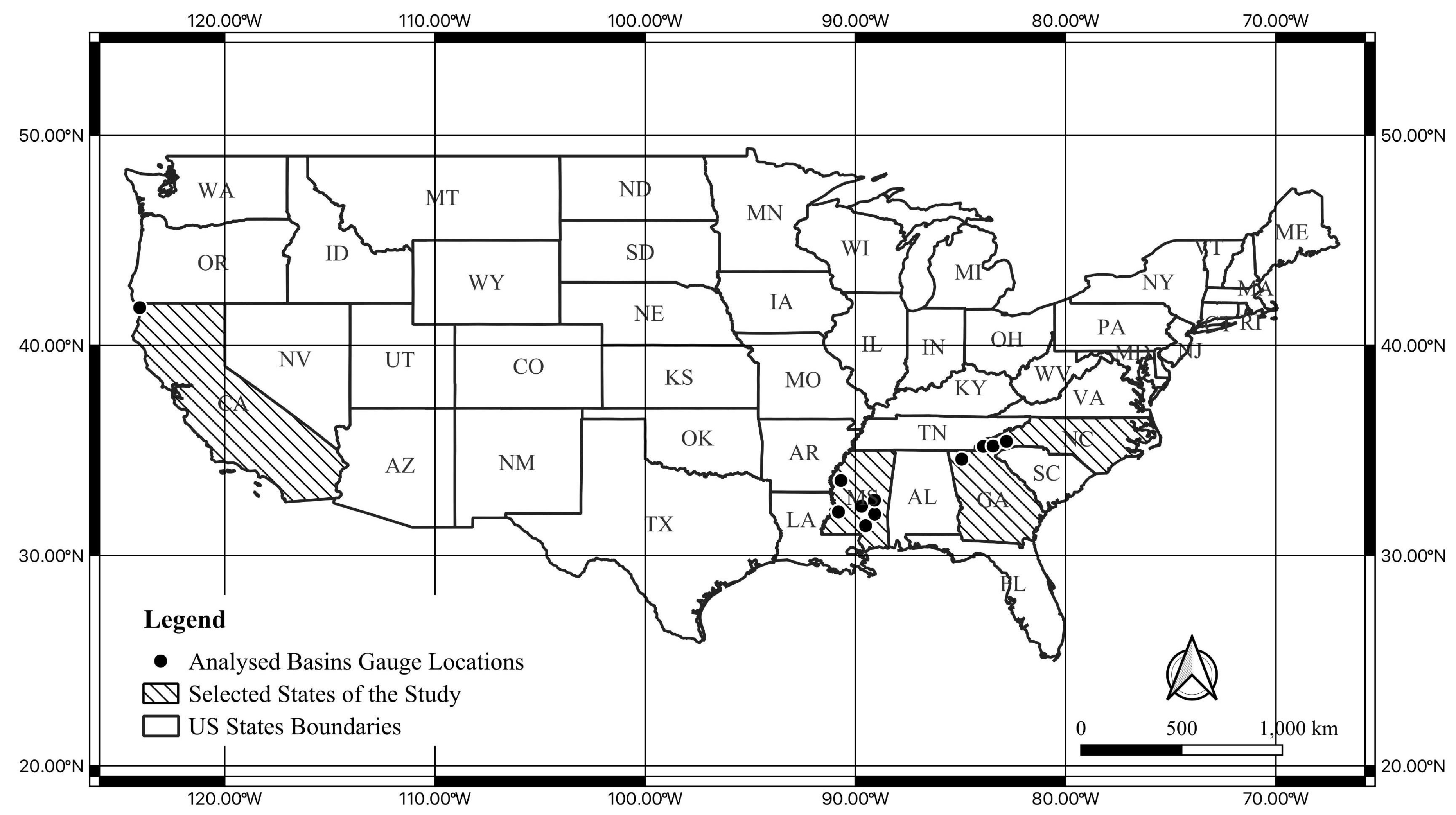
2.1. Study Basins

Five river basins in the USA were investigated during this study, including the same two basins from the recent study [36], as illustrated in Figure 1. The selection was based on the 30-year climate normal (1981–2010) released by NOAA’s National Climatic Data Centre (NCDC). The selection of the study basins was originally considered in accordance with the previous experiences in calibrating the XAJ model by Rahman and Lu (2015) [34] and Zin and Lu (2022) [36]. According to the studies [33,34,36,41,42], these basins possess robust datasets, and the XAJ model could accurately estimate their runoff. Therefore, this study attempted to utilize the study basin (MOPEX ID: 903504000, MOPEX ID: 902387500, MOPEX ID: 902472000, MOPEX ID: 903443000, and MOPEX ID: 911532500) to focus on the sensitivity of the recession constant over model performance in data-scarce areas. With the assessment including the same two basins permits comparing the parameter optimization and the minimum data length estimation from two different approaches. Furthermore, it provides a way to correlate the relationship between parameter sensitivity and model performance. Table 1 illustrates a brief overview of the physical characteristics of the researched basins.

2.2. Data Description

The U.S. MOPEX dataset [43] was employed to develop the basin scale daily precipitation P (daily mean aerial precipitation calculated from ground-based gauge precipitation), potential evaporation Ep (developed from NOAA Evaporation Atlas), and discharge Q (developed from USGS hydro-climatic data) information utilized in this research. Table 2 presents comprehensive descriptive data statistics of the examined basins.
Considering the lack of data and limitations in practical modeling research, the XAJ model is calibrated using the 28-year dataset and subsets from each basin to assess the model’s effectiveness. For the subsets, the 28-year dataset is divided into shorter data lengths with different year intervals starting from 6-year to 28-year subsets [36].
Here, we defined the input datasets In,m, including P and Ep, and Q o b s n , m as the observed runoff, where n is the length of datasets and m is the number of subsets ( m = 1 , 2 , , 28 n + 1 ).

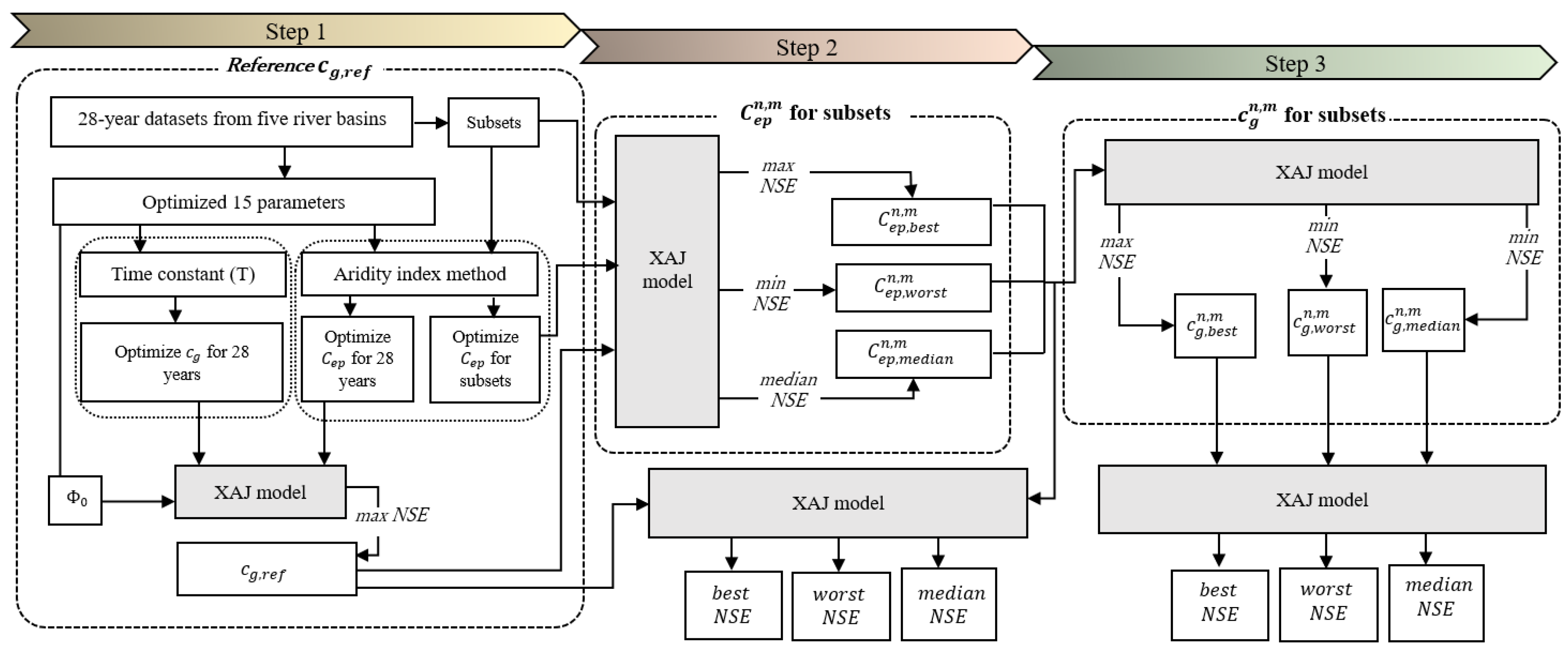
2.3. Analytical Framework of the Study

The analytical framework of this study comprises three steps as indicated in Figure 2.
Step 1:
Involves the selection of the XAJ model, followed by parameter optimization and calibration using a 28-year dataset to estimate the reference recession constant (cg,ref).
Step 2:
Encompasses the calculation and evaluation of the Cep values for each subset, and C e p n , m is achieved through the model calibration with cg,ref.
Step 3:
Outlines the procedure for evaluating the recession constant for the subsets, c g n , m . The evaluation is based on the model output obtained while running with C e p n , m .
A detailed explanation of each step will be provided in the subsequent sections.

2.4. Description of XAJ Model and Its Parameters

In this study, we utilized the Xinanjiang model, a conceptual hydrological model, developed by the Flood Forecast Research Institute of the East Chinese Technical University of Water Resources [44]. This model is originally designed for humid and semi-humid areas of China to estimate runoff generation within a basin [33,44]. In addition, it has proven effective in estimating in dry basins as discussed in Section 1 [37]. The model also demonstrates robust physical characteristics.

2.4.1. Selection and Calibration of Model Parameters

The simulated XAJ model utilized in this research comprises fifteen parameters, as detailed in Table 3 [44,45,46]. The complexity arising from the connections and interactions among the numerous parameters required in calibration can be minimized by the level of parameter estimation. Li and Lu [47] conducted the sensitivity of the XAJ model parameters at different time scales using the sensitivity analysis techniques by Morris [48]. This study reveals that the sensitivity of the XAJ model parameters varies across annual, monthly, and daily time scales. It can be categorized into the following groups:
Group 1:
Data adjustment parameters, sensitive on the annual scale.
Group 2:
Runoff component separation and routing-controlling parameters, sensitive on the daily scale.
Group 3:
Runoff generation-controlling parameters, sensitive on the annual scale while the Group 1 parameters are kept constant.

2.4.2. Relationship between Data Adjustment Parameter (Cep) and Recession Constant (cg)

The data adjustment parameter and linear reservoir recession are common parts in many widely used hydrological models, e.g., the NWS River Forecast System-Catchment Modeling and TANK model [49]. According to Lu and Li [33], the sensitivity of the variables impacting runoff generation (cg) appears sensitive yet again on an annual scale in the XAJ model while maintaining Cp and Cep as constant. Nevertheless, the recent study [36] mainly explored the impact of the sensitivity of the data adjustment parameter (Group 1) over the parameter estimation and model performance, applying both longer datasets and subsets. Therefore, the impact of recession constant sensitivity over the data adjustment parameter, especially during a period of data scarcity, needed to be considered.
According to the general water balance equation for the vertical water flux, the relationship between the adjustment parameter and the recession constant parameter can be observed as shown in the following equation:
C p P g = C e p E p + R + Δ S
where Pg is the actual rainfall calculated from a single rain gauge, Ep is the annual evaporation, R is the annual runoff depth, and Δ S is the changes in the water storage.
However, in this study, we considered that the baseflow storage can be affected by the recession constant cg at the beginning and end of the year under certain circumstances. To resolve this approach, Δ S must be taken into consideration, which is a highly subjective task that might have significant effects on the close relationship between Cep and cg.

2.4.3. Assessment of Data Adjustment Parameter (Cep)

Here, the estimation of the data adjustment parameter, Cep, is detailed through the aridity index method emphasized by Li and Lu [41]. According to that, correlating the runoff coefficient and data aridity index could support the reduction in the parameter space for Cp and Cep rather than separate assessments. Therefore, to reduce such an inaccuracy and improve the efficiency of parameter estimation, the interaction between the runoff coefficient and the data aridity index is applied to parameter estimation.
Within the limitations of the pan aridity index ( ζ g , p a n ) and annual runoff coefficient (R/Pg), the values of Cp and Cep might be determined by the following logarithmic form [41],
ln ( R / P g ) = α ( C e p / C p ) ζ g , p a n + ln C p
Here, estimation for the 28-year dataset and subsets is outlined by function Y, and C e p n , m represent the estimated Cep values for the subsets, In,m. The subsequent equation explains the data adjustment parameter estimation in the subsets, In,m.
C e p n , m = Y ( Q o b s n , m , I n , m )

2.4.4. Assessment of Recession Constant (cg)

Three runoff components [33] consisting of the surface runoff, interflow, and baseflow are routed using three linear reservoirs as follows:
Q x t + 1 = c x Q x t + 1 c x R x x = s , i , g
where subscript x indicates the runoff component, s is for the surface flow, i is for the interflow, and g is for the baseflow; cs, ci, and cg are their recession coefficients. Usually,
0   <   c s   <   c i   <   c g   <   1
Based on the related literature [33], among the 15 parameters in the XAJ model, the most sensitive parameter at the annual scale when keeping the data adjustment parameters constant is cg. Therefore, this study introduced the sensitivity of cg over the data adjustment parameters. The recession constant values were initially calculated based on the time constant, T, not to exceed the limits between 0 and 1. T is related to cg by the following expression,
T = Δ t   / ln c g
whereas T is the time constant of the baseflow system in days, and cg is the recession constant in a t dimensionless quantity whose value depends on the time unit chosen (days).

2.4.5. XAJ Model Calibration

To implement Step 1 in Figure 2, let the function specify the XAJ model calibration, X, and let the input datasets comprise the vector In,m. Let the simulated runoff, Q c a l n , m , via the XAJ model calibration for In,m, be specified by the following equation:
Q c a l n , m = X ( I n , m , C e p , c g ϕ 0 )
where Cep represents the adjustment parameter (the most sensitive parameter at the annual scale in the XAJ model), cg is the recession constant (sensitive at the annual scale when the adjustment parameters are kept constant), and ϕ 0 represents the application of 13 pre-optimized parameter values, which is a subset of all 15 parameters in the XAJ model as in Table 2. These parameters are fixed in this study. As these parameter values are not inferred through the calibration process, ϕ 0 will be excluded from the following equation for clarity.
Q c a l n , m = X ( I n , m , C e p , c g )

2.4.6. Evaluation of Model Performance Using Nash–Sutcliffe Efficiency

The Nash and Sutcliffe (1970) coefficient of efficiency is widely used in the evaluation of hydrological modeling [50,51,52,53,54,55]. Simulated runoff information is derived utilizing the well-known Nash–Sutcliffe efficiency [56].
The definition of the Nash–Sutcliffe efficiency is as follows:
N S E = 1 t = 1 n Q o b s t Q c a l t 2 t = 1 n Q o b s t Q o b s ¯ 2
where Qcal is the simulated runoff, Qobs is the observed runoff, and Q o b s ¯ is the mean value of the observed runoff.
This study calculates the observed and simulated runoff from the XAJ model driven by the subsets, In,m. It can be expressed as follows:
N S E n , m = N S E ( Q o b s n , m , Q c a l n , m )
where Q o b s n , m is the daily observed runoff.
At an annual scale, the parameters affecting the Q c a l n , m are mainly Cep and cg. Thus, Equation (9) can also be written in the following function:
N S E n , m = N S E ( C e p n , m , c g n , m Q o b s n , m , ϕ 0 ) = N S E ( C e p n , m , c g n , m )

2.4.7. Estimation of Reference Recession Constant (cg,ref)

The simulated recession constant, cg,ref, is initially estimated by comparing the model results using the linear polynomial regression analysis. The values of cg,ref were selected based on the cg values with the best model performance in the longest datasets (Figure 2).
N S E ( C e p 28 , 1 , c g , r e f ) N S E ( C e p 28 , 1 , c g )
where C e p 28 , 1 refers to the estimated adjustment parameter value using a 28-year data length.

2.5. Estimation of C e p n , m for Subsets

To highlight the sensitivity impact of the recession constant in shorter datasets, the data adjustment parameter values for the subsets are essential to optimize the recession constant values for the subsets as indicated in Step 2 of Figure 2. To compare the impacts of the parameter sensitivity in a shorter data length, we first identify the estimated Cep values for the subsets based on three conditions: the maximum, minimum, and median annual model results, NSE. Let C e p , b e s t n , m , C e p , w o r s t n , m , and C e p , m e d i a n n , m be the maximum, minimum, and median C e p n , m values in the subsets (In,m), when running the model using cg,ref.
The maximum, minimum, and median annual NSE can be specified using C e p n , m and cg,ref in the subsets by using the following equations:
m a x ( N S E ( C e p n , m , c g , r e f ) ) = N S E ( C e p , b e s t n , m , c g , r e f )
m i n ( N S E ( C e p n , m , c g , r e f ) ) = N S E ( C e p , w o r s t n , m , c g , r e f )
m e d i a n ( N S E ( C e p n , m , c g , r e f ) ) = N S E ( C e p , m e d i a n n , m , c g , r e f )

2.6. Estimation of c g n , m for Subsets

For the comparison of the sensitivity influence of the recession constants over the parameter estimation in a shorter data length, we apply the maximum, minimum, and median calibrated data adjustment parameter values ( C e p , b e s t n , m , C e p , w o r s t n , m , and C e p , m e d i a n n , m ) in the model calibration to receive the maximum, minimum, and median recession constant values ( c g , b e s t n , m , c g , w o r s t n , m , and c g , m e d i a n n , m ) in the subsets (refer to Step 3 in Figure 2).

2.7. Comparative Evaluation of Recession Constant Sensitivity in Subsets

Finally, the maximum, minimum, and median annual NSE results using c g , b e s t n , m , c g , w o r s t n , m , and c g , m e d i a n n , m are estimated by comparing the NSE results calibrated with cg,ref using the following equations:
N S E ( C e p , b e s t n , m , c g , b e s t n , m ) N S E ( C e p , b e s t n , m , c g , r e f )
N S E ( C e p , w o r s t n , m , c g , w o r s t n , m ) N S E ( C e p , w o r s t n , m , c g , r e f )
N S E ( C e p , m e d i a n n , m , c g , m e d i a n n , m ) N S E ( C e p , m e d i a n n , m , c g , r e f )
where c g , b e s t n , m , c g , w o r s t n , m , and c g , m e d i a n n , m are calculated based on the maximum, minimum, and median model outputs while running C e p , b e s t n , m , C e p , w o r s t n , m , and C e p , m e d i a n n , m with cg,ref.

2.8. Application of Linear Polynomial Regression Analysis for Data Comparison

In this study, a polynomial regression analysis was applied to attain and analyze the relationship between cg and the annual Nash using both of them and the subsets to access the best approximation between these two parameter values [57,58].

3. Results and Discussion

The impact of limited data on parameter estimation stands out as a pivotal factor influencing both the reliability and precision of the model. Thus, in designing long-term hydrological models, the time-related character of sensitivity becomes critical [59]. For effective calibration and predictions during a period of data scarcity, the XAJ model has its limitations. Challenges in calibration and validation arise from restricted calibration data for accurate parameter estimation, insufficient data for robust model predictions, the impact on parameter sensitivity with spatial and temporal variation, increased uncertainties within the model performance due to data scarcity, and potential over-parameterizations. Consequently, it is necessary to consider the influence of sensitive parameters on the XAJ model performance when there are data limitations.
A recent study [36] has indicated that the performance of the data adjustment parameter (the most sensitive parameter at the annual scale) estimation is enhanced with longer datasets. As illustrated in Figure 3, it is evident that there is considerable variation in the optimization of the data adjustment parameter values in shorter datasets. In a recent study, Lu and Li [33] proved that the variables impacting runoff generation (cg) appear sensitive yet again on an annual scale in the XAJ model while maintaining Cp and Cep as constant. Based on this finding, this study attempted to analyze the sensitivity of recession constant estimation in accordance with the data adjustment parameter during the period of data scarcity. Consequently, understanding the sensitivity of the recession constant over the model performance becomes critical.
To emphasize the sensitivity of the recession constant, the XAJ model calibration was conducted through two approaches, as detailed in Figure 2. First, the model was calibrated and evaluated using reference recession constant values (cg,ref) optimized with longer datasets. Second, the model performance was accessed and compared using the recession constant for the subsets ( c g n , m ).

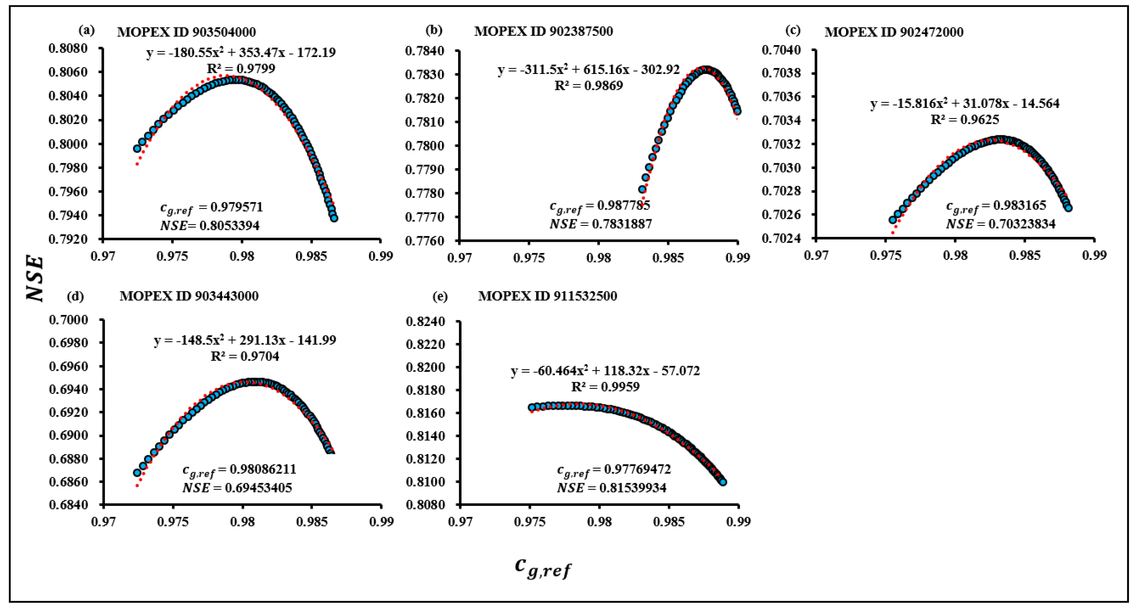
3.1. Reference cg for 28-Year Datasets (cg,ref)

The pre-optimized recession constant values in the five MOPEX studied basins were initially computed based on the time constant, T, as in Equation (5), to be achieved within the interval [0,1]. These resulting cg values were incorporated into the XAJ model calibration alongside the remaining pre-optimized parameters, ϕ 0 . Utilizing the annual Nash results, the estimation of the simulated cg for each basin was assessed through a polynomial regression analysis.
Typically, to attain better calibration, model users employ the longest available data series. In this study, the simulated recession constant, estimated using a 28-year dataset, was employed as the reference. Nevertheless, the purpose of this study is to analyze the sensitivity of the recession constant during a period of data limitations to highlight its impact on the parameter calibration and model performance [26,60]. Consequently, it becomes essential to estimate the recession constant values in the shorter datasets. To address this, the optimization of the Cep values ( C e p n , m ) for shorter datasets is essential for the consideration of the recession constant values for the subsets. Figure 4 reveals the estimation of cg,ref, by comparing the annual Nash, NSE, calculated using the pre-optimized cg values.

3.2. Derivation of Data Adjustment Parameter ( C e p n , m )

To assess the sensitivity of the recession constant over the data adjustment parameter for consecutive subsets (In,m), it was crucial to optimize the data adjustment parameter values, C e p n , m , for the subsets by applying cg,ref.
The values of C e p n , m for the subsets (see Figure 5) were classified into three categories based on the model (NSE) values calibrated using the reference cg,ref in each subset, In,m:
(i)
C e p , b e s t n , m (selected when the annual Nash values, NSE, are highest after the model calibration with cg,ref in each subset, In,m);
(ii)
C e p , m e d i a n n , m (selected when the annual Nash values, NSE, are median after the model calibration with cg,ref in each subset, In,m);
(iii)
C e p , w o r s t n , m (selected when the annual Nash values, NSE, are lowest after the model calibration with cg,ref in each subset, In,m).
Subsequently, the polynomial regression analysis was conducted to determine the corresponding c g n , m for the subsets in each category ( c g , b e s t n , m , c g , m e d i a n n , m , and c g , w o r s t n , m ) respectively.

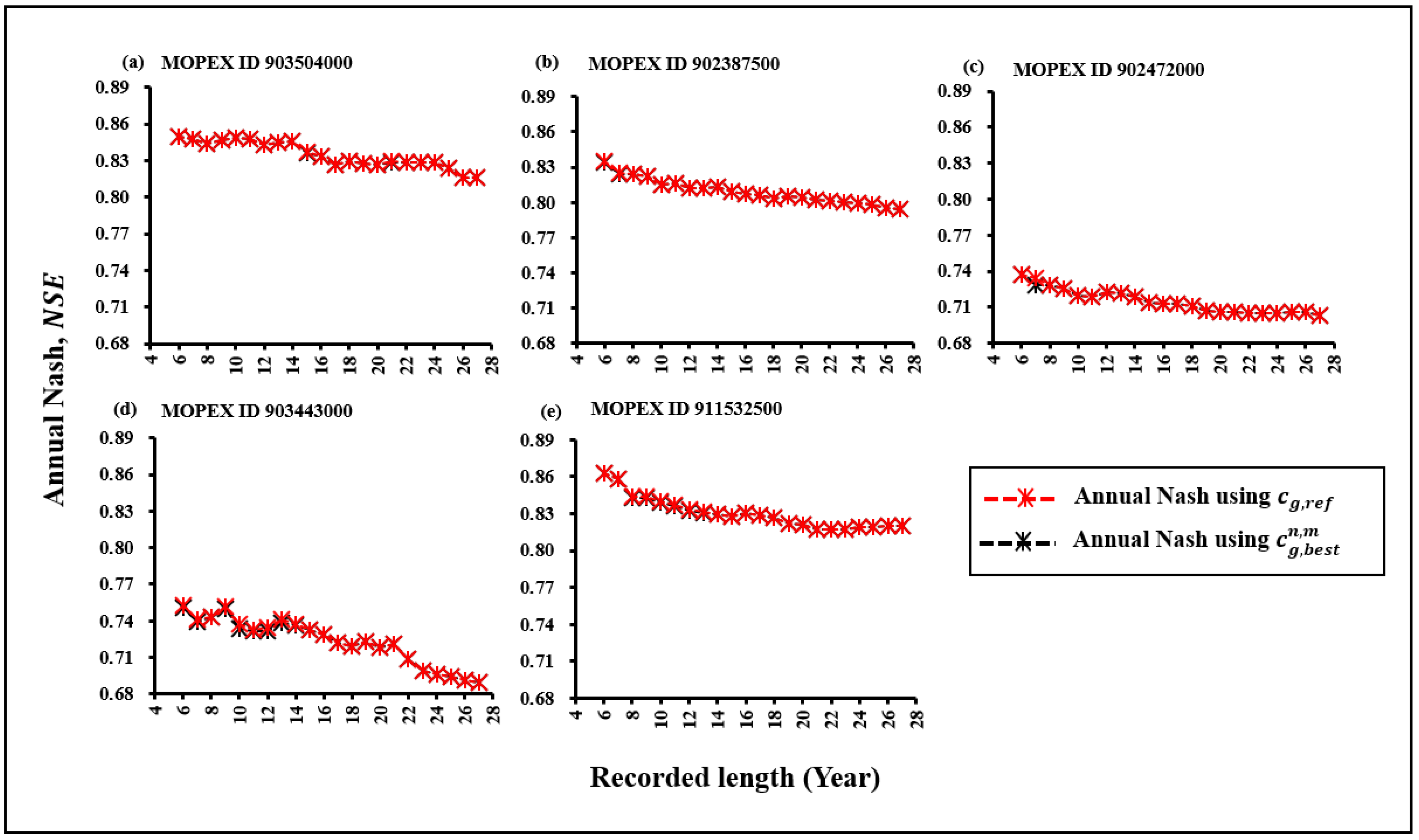
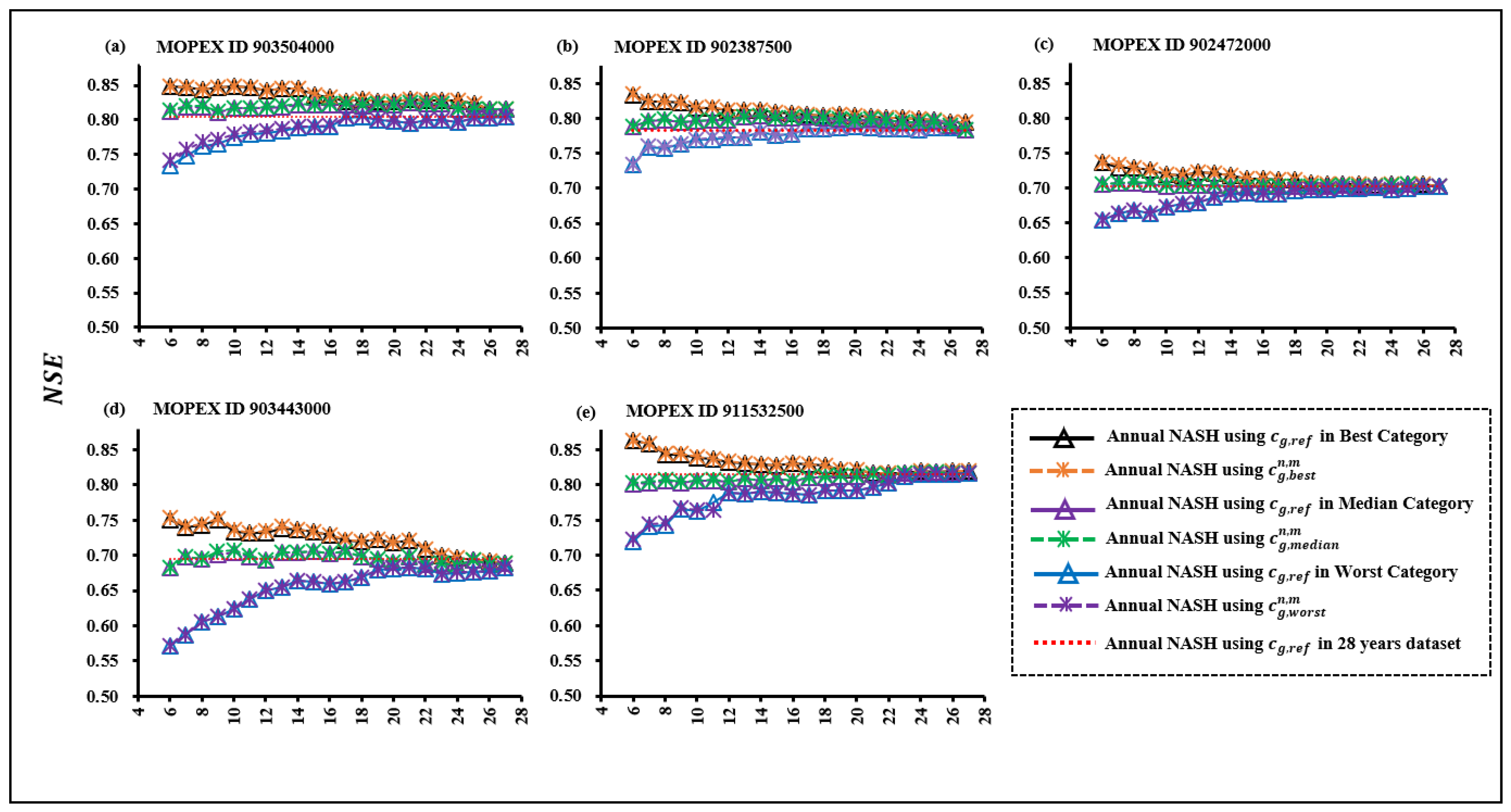
3.3. Comparative Evaluation of Annual Nash Results, NSE, Using c g , b e s t n , m and C e p , b e s t n , m in Subsets

After the model calibration using the reference cg, the Cep ( C e p , b e s t n , m ) corresponding to the highest annual Nash results were selected and calibrated for c g , b e s t n , m optimization (see Figure 6).
Figure 7 represents the results of the NSE values for both cg,ref and c g , b e s t n , m . As depicted in Figure 7, it was observed that as the data length increases, both NSE values compared from both cg,ref and c g , b e s t n , m exhibit a declining trend. This suggests that longer datasets might face challenges aligning with the model’s best performance. In contrast, the 6-year subsets displayed the most significant upward trends in both NSE results, which was attributed to shorter datasets being more compatible with c g , b e s t n , m . Beyond this trend pattern, a comparison was conducted between the NSE values in the subsets while conducting this with cg,ref and c g , b e s t n , m .
Figure 7 illustrates that the NSE values in each subset exhibited a relative increase when running the model with c g , b e s t n , m . However, no significant difference was observed with the NSE resulting from the model calibration using both cg,ref and c g , b e s t n , m . As indicated in Figure 8, the percentage of the relative difference in the NSE values between c g , r e f and c g , b e s t n , m in the case of the 6-year datasets was 0.000243 for MOPEX ID: 903504000, 0.117651 for MOPEX ID: 902387500, 0.001037 for MOPEX ID: 902472000, 0.264031 for MOPEX ID: 903443000, and 0.048047 for MOPEX ID: 911532500, respectively. It is clear that the results exhibit marginal sensitivity to the model performance during the calibration with c g , b e s t n , m , indicating limited space for improving the model performance as illustrated in Figure 7. Given the results, it is likely that the impact of the sensitivity of c g , b e s t n , m over Cep in parameter estimation in shorter datasets can also be considered limited. Consequently, the potential impact of the sensitivity of c g , b e s t n , m can also be limited to the performance of the model as well as the minimum data length estimation. On the other hand, the recent estimation of the minimum data length remains consistent while considering the sensitivity of the parameter estimation with cg in the best parameter optimization scenario within the subsets.

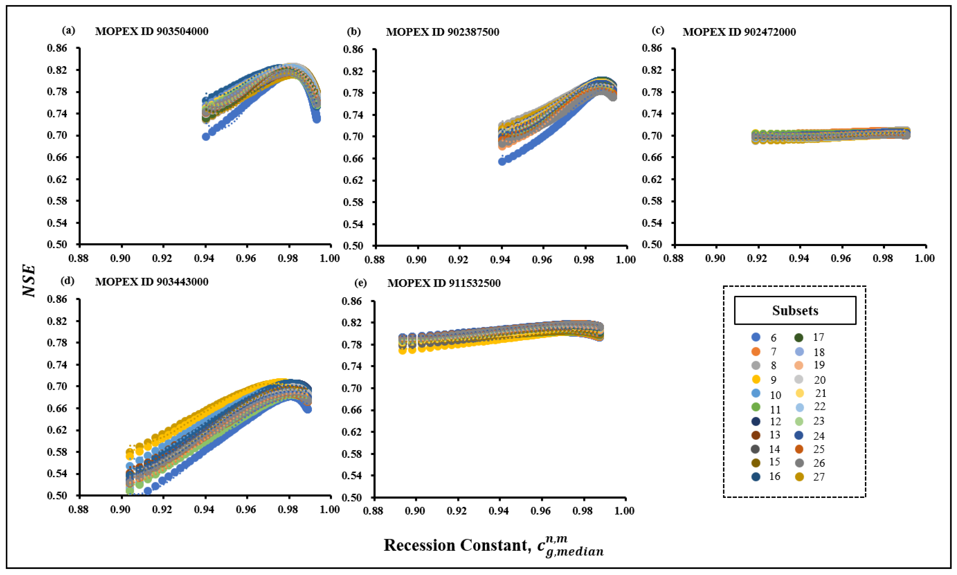
3.4. Comparative Evaluation of Annual Nash Results, NSE, Using c g , m e d i a n n , m and C e p , m e d i a n n , m in Subsets

In this section, the values of Cep ( C e p , m e d i a n n , m ) were selected based on the median values of the model output (NSE) following the model calibration with cg,ref for the 28-year datasets. Subsequent to the C e p , m e d i a n n , m selection using the model outputs with cg,ref, the model calibration was executed to establish the relationship between the NSE and the c g , m e d i a n n , m results. In Figure 9, the c g , m e d i a n n , m can be approximated by the model output (NSE) using the linear polynomial regression analysis. Here, while taking the cg values in the median range, the trend resulting from both NSE values using cg,ref and c g , m e d i a n n , m for all the studied basins has slightly increased as the data length increased.
While considering the cg values within the median parameter optimization performance scenario, the NSE values exhibited a slight upward trend across all the subsets as the data length increased. Furthermore, the NSE values when utilizing c g , m e d i a n n , m were slightly higher than those with cg,ref. In this case, the percentage of the relative difference in the NSE values from cg,ref and c g , m e d i a n n , m in the 6-year subsets can be observed as 0.143159 for MOPEX ID: 903504000, 0.111729 for MOPEX ID: 902387500, 0.001622 for MOPEX ID: 902472000, 0.231673 for MOPEX ID: 903443000, and 0.152241 for MOPEX ID: 911532500, respectively (see Figure 8). This demonstrates that some of the differences resulted in the best-case scenario. Despite this minor difference, it is reasonable to conclude that the model outcomes using median values did not indicate a considerable amount of limitations over the model performance while calibrating during the period of data scarcity as indicated in Figure 10.

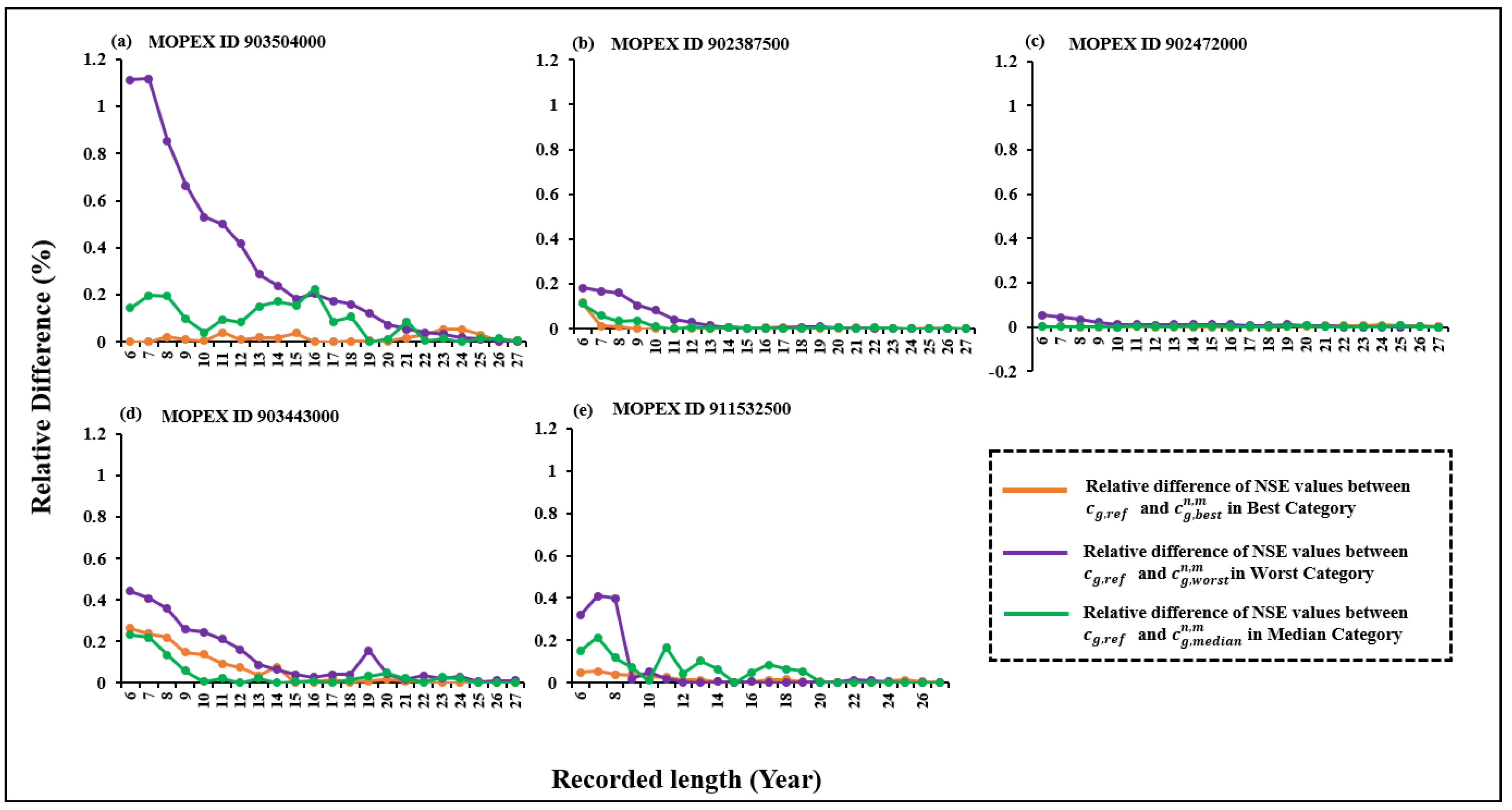
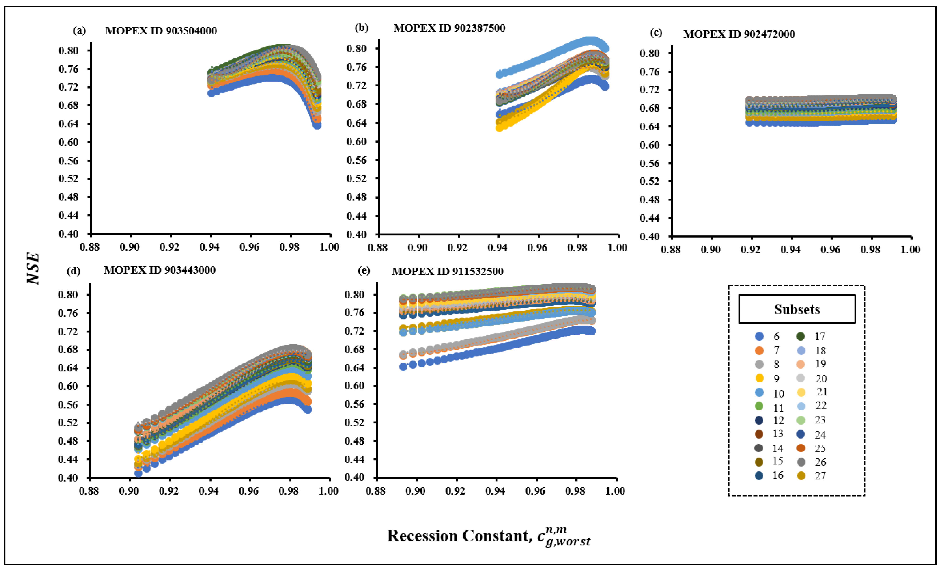
3.5. Comparative Assessment of Annual Nash Results, NSE, Using c g , w o r s t n , m and C e p , w o r s t n , m in Subsets

According to Li and Lu [47], to estimate the most sensitive parameter, it can be considered both the best and worst condition for the sensitivity analysis for the parameter optimization. However, to expect good model performance, the worst condition for the parameter optimization is essential to take into consideration. This approach to achieving strong model performance under challenging conditions is imperative. Figure 11 reveals the values of c g , w o r s t n , m optimized from the C e p , w o r s t n , m values described in Table 4.
Compared to the model performances in the best-case and median-case scenarios, a significant difference is evident with those from c g , w o r s t n , m and cg,ref (see Figure 12). The percentage of the relative difference in the NSE values in each basin for the 6-year datasets is 1.111107 for MOPEX ID: 903504000, 0.183231 for MOPEX ID: 902387500, 0.053648 for MOPEX ID: 902472000, 0.442889 for MOPEX ID: 903443000, and 0.320853 for MOPEX ID: 911532500, respectively. However, the relative difference between the NSE results calibrated using cg,ref and c g , w o r s t n , m decreases gradually when running the model with longer datasets in all the study basins. This result showed there is a comparatively high relative difference in the NSE values and highlighted the significant impact over the model performance by utilizing the NSE values with c g , w o r s t n , m in the shorter datasets in all the study basins.
Unlike the previously mentioned categories, the influence of cg on the estimation of Cep becomes pronounced in the worst-case scenario (Figure 8). Additionally, the sensitivity of cg further magnifies its impact on model performance under these conditions. The insight provided by Figure 13 and Figure 8 clearly illustrates the variations in the NSE values among the three categories across all the studied basins.

4. Conclusions

A recent study explored the impact of data adjustment parameter estimation on model performance in data-scarce regions. Given the common use of the data adjustment parameter and recession constant in hydrological modeling, it is crucial to assess the influence of recession constant sensitivity over the data adjustment parameter, particularly during a period of data scarcity.
Utilizing a linear polynomial regression analysis on the 28-year U.S. MOPEX datasets and subsets from five river basins, this study considered parameter optimization, focusing on the estimation of the recession constant and data adjustment parameter values calculated using the aridity index method and the time constant using the XAJ model. Multiple steps of parameter optimization were executed for parameter estimation in the shorter subsets, and the resulting model outputs were evaluated using Nash–Sutcliffe efficiency (NSE) values.
A data analysis based on the relative difference method revealed that the potential impact of the recession constant and its interaction with the data adjustment parameter is limited in longer datasets. Investigating the shorter datasets based on three scenarios, the study highlights that recession constant sensitivity has limited potential to enhance model performance in best and median scenarios. In contrast, while recession constant sensitivity moderately influences model performance in shorter datasets, a notable difference in model performance is evident, particularly within a 12-year minimum data length, under the worst-case scenario in all the study basins.
This finding underscores the crucial role of recession constant sensitivity in parameter optimization, especially during a period of limited data availability where the parameter optimization is not in a favorable condition. The analysis demonstrates the robust relationship between the recession constant parameter and the data adjustment parameter across varying data lengths in longer datasets. Importantly, the study emphasizes the necessity of considering recession constant sensitivity in shorter datasets, particularly in basins with restricted data availability, where it can significantly impact model performance, especially under worst-case scenarios.
This research offers valuable insights applicable beyond the realm of the XAJ model, extending its relevance to various hydrological modeling approaches. This study did not consider the basin characteristics and the geology. Despite the limitations (the XAJ model performance under the data limitations) and assumption (an exclusive focus on annual scale sensitivity instead of seasonal assessment and the statistical significance), this study contributes insights into the influence of recession constant sensitivity in parameter estimation and its importance in developing countries with limited data availability for robust model predictions. This, in turn, aids in determining precise and acceptable minimum data length estimations, particularly in regions with limited data availability, such as developing countries.

Author Contributions

Conceptualization, T.T.Z. and M.L.; methodology, T.T.Z. and M.L.; software, T.T.Z. and T.O.; validation, T.T.Z. and M.L.; formal analysis, T.T.Z. and M.L.; investigation, T.T.Z. and M.L.; resources, M.L.; data curation, T.T.Z.; writing—original draft preparation, T.T.Z.; writing—review and editing, T.T.Z. and M.L.; visualization, T.T.Z.; supervision, M.L.; project administration, M.L; funding acquisition, M.L. All authors have read and agreed to the published version of the manuscript.

Funding

This research received no external funding.

Data Availability Statement

Information on all the data applied in this research is shown in Section 2.

Conflicts of Interest

Regarding this paper and the research, the authors state that they have no conflicts of interest.

Abbreviations

The following abbreviations are used in this paper:
XAJXinanjiang model
C e p Data adjustment parameter
c g Recession constant
ζ g , p a n Pan aridity index
nLength of datasets
mNumber of subsets
TTime constant
C e p 28 , 1 Data adjustment parameter for 28-year data length
C e p n , m Data adjustment parameter for subsets
ϕ 0 Thirteen pre-optimized parameter values
C e p , b e s t n , m Data adjustment parameter with maximum NSE for subsets
C e p , m e d i a n n , m Data adjustment parameter with median NSE for subsets
C e p , m i n i m u m n , m Data adjustment parameter with minimum NSE for subsets
c g , r e f Reference recession constant
c g n , m Recession constant for subsets
c g , b e s t n , m Recession constant with maximum NSE for subsets
c g , m e d i a n n , m Recession constant with median NSE for subsets
c g , m i n i m u m n , m Recession constant with minimum NSE for subsets
PDaily precipitation
E p Potential evaporation
RAnnual runoff depth
SWater storage
I n , m Input datasets
Q o b s n , m Observed runoff
Q c a l n , m Simulated runoff
NSENash–Sutcliffe efficiency

References

  1. Devia, G.K.; Ganasri, B.P.; Dwarakish, G.S. A review on hydrological models. Aquat. Procedia 2015, 4, 1001–1007. [Google Scholar] [CrossRef]
  2. Peel, M.C.; Blöschl, G. Hydrological modelling in a changing world. Prog. Phys. Geogr. 2011, 35, 249–261. [Google Scholar] [CrossRef]
  3. Birkholz, S.; Muro, M.; Jeffrey, P.; Smith, H.M. Rethinking the relationship between flood risk perception and flood management. Sci. Total Environ. 2014, 478, 12–20. [Google Scholar] [CrossRef] [PubMed]
  4. Adikari, Y.; Yoshitani, J. Global Trends in Water-Related Disasters: An Insight for Policymakers; World Water Assessment Programme Side Publication Series, Insights; The United Nations, UNESCO: London, UK; International Centre for Water Hazard and Risk Management (ICHARM): Ibaraki-ken, Japan, 2009; pp. 1–24. [Google Scholar]
  5. Modarres, R.; Ouarda, T.B. Modeling rainfall–runoff relationship using multivariate GARCH model. J. Hydrol. 2013, 499, 1–18. [Google Scholar] [CrossRef]
  6. Hamilton, S. Completing the loop: From data to decisions and back to data. Hydrol. Process. 2007, 21, 3105–3106. [Google Scholar] [CrossRef]
  7. Loucks, D.P.; Van Beek, E. Water Resource Systems Planning and Management: An Introduction to Methods, Models, and Applications; Springer: Berlin/Heidelberg, Germany, 2017. [Google Scholar]
  8. Refsgaard, J.C.; Knudsen, J. Operational validation and intercomparison of different types of hydrological models. Water Resour. Res. 1996, 32, 2189–2202. [Google Scholar] [CrossRef]
  9. Ramos, M.H.; Mathevet, T.; Thielen, J.; Pappenberger, F. Communicating uncertainty in hydro-meteorological forecasts: Mission impossible? Meteorol. Appl. 2010, 17, 223–235. [Google Scholar] [CrossRef]
  10. Raje, D.; Krishnan, R. Bayesian parameter uncertainty modeling in a macroscale hydrologic model and its impact on Indian river basin hydrology under climate change. Water Resour. Res. 2012, 48. [Google Scholar] [CrossRef]
  11. Zhao, F.; Wu, Y.; Qiu, L.; Sun, Y.; Sun, L.; Li, Q.; Niu, J.; Wang, G. Parameter uncertainty analysis of the SWAT model in a mountain-loess transitional watershed on the Chinese Loess Plateau. Water 2018, 10, 690. [Google Scholar] [CrossRef]
  12. Wu, Y.; Liu, S.; Huang, Z.; Yan, W. Parameter optimization, sensitivity, and uncertainty analysis of an ecosystem model at a forest flux tower site in the United States. J. Adv. Model. Earth Syst. 2014, 6, 405–419. [Google Scholar] [CrossRef]
  13. Bárdossy, A.; Singh, S. Robust estimation of hydrological model parameters. Hydrol. Earth Syst. Sci. 2008, 12, 1273–1283. [Google Scholar] [CrossRef]
  14. Gupta, H.V.; Sorooshian, S.; Yapo, P.O. Status of automatic calibration for hydrologic models: Comparison with multilevel expert calibration. J. Hydrol. Eng. 1999, 4, 135–143. [Google Scholar] [CrossRef]
  15. McMillan, H.; Clark, M. Rainfall-runoff model calibration using informal likelihood measures within a Markov chain Monte Carlo sampling scheme. Water Resour. Res. 2009, 45. [Google Scholar] [CrossRef]
  16. Gou, J.; Miao, C.; Duan, Q.; Tang, Q.; Di, Z.; Liao, W.; Wu, J.; Zhou, R. Sensitivity analysis-based automatic parameter calibration of the VIC model for streamflow simulations over China. Water Resour. Res. 2020, 56, e2019WR025968. [Google Scholar] [CrossRef]
  17. Renard, B.; Kavetski, D.; Kuczera, G.; Thyer, M.; Franks, S.W. Understanding predictive uncertainty in hydrologic modeling: The challenge of identifying input and structural errors. Water Resour. Res. 2010, 46. [Google Scholar] [CrossRef]
  18. Muleta, M.K.; Nicklow, J.W. Sensitivity and uncertainty analysis coupled with automatic calibration for a distributed watershed model. J. Hydrol. 2005, 306, 127–145. [Google Scholar] [CrossRef]
  19. Jeremiah, E.; Sisson, S.A.; Sharma, A.; Marshall, L. Efficient hydrological model parameter optimization with Sequential Monte Carlo sampling. Environ. Model. Softw. 2012, 38, 283–295. [Google Scholar] [CrossRef]
  20. Celeux, G.; Hurn, M.; Robert, C.P. Computational and inferential difficulties with mixture posterior distributions. J. Am. Stat. Assoc. 2000, 95, 957–970. [Google Scholar] [CrossRef]
  21. Bates, B.C.; Campbell, E.P. A Markov chain Monte Carlo scheme for parameter estimation and inference in conceptual rainfall-runoff modeling. Water Resour. Res. 2001, 37, 937–947. [Google Scholar] [CrossRef]
  22. Vrugt, J.A.; Ter Braak, C.J.; Clark, M.P.; Hyman, J.M.; Robinson, B.A. Treatment of input uncertainty in hydrologic modeling: Doing hydrology backward with Markov chain Monte Carlo simulation. Water Resour. Res. 2008, 44. [Google Scholar] [CrossRef]
  23. Gottschalk, F.; Sun, T.; Nowack, B. Environmental concentrations of engineered nanomaterials: Review of modeling and analytical studies. Environ. Pollut. 2013, 181, 287–300. [Google Scholar] [CrossRef]
  24. Kuczera, G.; Parent, E. Monte Carlo assessment of parameter uncertainty in conceptual catchment models: The Metropolis algorithm. J. Hydrol. 1998, 211, 69–85. [Google Scholar] [CrossRef]
  25. Micevski, T.; Kuczera, G. Combining site and regional flood information using a Bayesian Monte Carlo approach. Water Resour. Res. 2009, 45. [Google Scholar] [CrossRef]
  26. Sorooshian, S.; Gupta, V.K. Automatic calibration of conceptual rainfall-runoff models: The question of parameter observability and uniqueness. Water Resour. Res. 1983, 19, 260–268. [Google Scholar] [CrossRef]
  27. Thyer, M.; Renard, B.; Kavetski, D.; Kuczera, G.; Franks, S.W.; Srikanthan, S. Critical evaluation of parameter consistency and predictive uncertainty in hydrological modeling: A case study using Bayesian total error analysis. Water Resour. Res. 2009, 45. [Google Scholar] [CrossRef]
  28. Wagener, T.; McIntyre, N.; Lees, M.; Wheater, H.; Gupta, H. Towards reduced uncertainty in conceptual rainfall-runoff modelling: Dynamic identifiability analysis. Hydrol. Process. 2003, 17, 455–476. [Google Scholar] [CrossRef]
  29. Pande, S.; Savenije, H.H.; Bastidas, L.A.; Gosain, A.K. A parsimonious hydrological model for a data scarce dryland region. Water Resour. Manag. 2012, 26, 909–926. [Google Scholar] [CrossRef]
  30. Nyeko, M. Hydrologic modelling of data scarce basin with SWAT model: Capabilities and limitations. Water Resour. Manag. 2015, 29, 81–94. [Google Scholar] [CrossRef]
  31. Bergström, S. Principles and confidence in hydrological modelling. Hydrol. Res. 1991, 22, 123–136. [Google Scholar] [CrossRef]
  32. Parajka, J.; Viglione, A.; Rogger, M.; Salinas, J.; Sivapalan, M.; Blöschl, G. Comparative assessment of predictions in ungauged basins–Part 1: Runoff-hydrograph studies. Hydrol. Earth Syst. Sci. 2013, 17, 1783–1795. [Google Scholar] [CrossRef]
  33. Lu, M.; Li, X. Time scale dependent sensitivities of the XinAnJiang model parameters. Hydrol. Res. Lett. 2014, 8, 51–56. [Google Scholar] [CrossRef]
  34. Rahman, M.M.; Lu, M. Model spin-up behavior for wet and dry basins: A case study using the Xinanjiang model. Water 2015, 7, 4256–4273. [Google Scholar] [CrossRef]
  35. Rahman, M.M.; Lu, M.; Kyi, K.H. Variability of soil moisture memory for wet and dry basins. J. Hydrol. 2015, 523, 107–118. [Google Scholar] [CrossRef]
  36. Zin, T.T.; Lu, M. Influence of Data Length on the Determination of Data Adjustment Parameters in Conceptual Hydrological Modeling: A Case Study Using the Xinanjiang Model. Water 2022, 14, 3012. [Google Scholar] [CrossRef]
  37. Gan, T.Y.; Dlamini, E.M.; Biftu, G.F. Effects of model complexity and structure, data quality, and objective functions on hydrologic modeling. J. Hydrol. 1997, 192, 81–103. [Google Scholar] [CrossRef]
  38. Beven, K.J. Rainfall-Runoff Modelling: The Primer; John Wiley & Sons: Hoboken, NJ, USA, 2011. [Google Scholar]
  39. Lu, M. Recent and future studies of the Xinanjiang Model. J. Hydraul. Eng. 2021, 52, 432–441. [Google Scholar]
  40. Gan, Y.; Duan, Q.; Gong, W.; Tong, C.; Sun, Y.; Chu, W.; Ye, A.; Miao, C.; Di, Z. A comprehensive evaluation of various sensitivity analysis methods: A case study with a hydrological model. Environ. Model. Softw. 2014, 51, 269–285. [Google Scholar] [CrossRef]
  41. Li, X.; Lu, M. Application of aridity index in estimation of data adjustment parameters in the Xinanjiang model. J. Jpn. Soc. Civ. Eng. Ser (Hydraul. Eng.) 2014, 70, I_163–I_168. [Google Scholar] [CrossRef]
  42. Rahman, M.M.; Lu, M.; Kyi, K.H. Seasonality of hydrological model spin-up time: A case study using the Xinanjiang model. Hydrol. Earth Syst. Sci. Discuss. 2016, prepirnt. [Google Scholar]
  43. Schaake, J.; Cong, S.; Duan, Q. US MOPEX Data Set; Technical Report; Lawrence Livermore National Lab. (LLNL): Livermore, CA, USA, 2006. [Google Scholar]
  44. Ren-Jun, Z. The Xinanjiang model applied in China. J. Hydrol. 1992, 135, 371–381. [Google Scholar] [CrossRef]
  45. Hapuarachchi, H.; Li, Z.; Wang, S. Application of SCE-UA method for calibrating the Xinanjiang watershed model. J. Lake Sci. 2001, 13, 304–314. [Google Scholar]
  46. Zhao, R.; Liu, X. Computer Models of Watershed Hydrology. In The Xinanjiang Model; Singh, V.P., Ed.; Water Resources Publications: Littleton, CO, USA, 1995. [Google Scholar]
  47. Li, X.; Lu, M. Multi-step optimization of parameters in the Xinanjiang model taking into account their time scale dependency. J. Jpn. Soc. Civ. Eng. Ser. (Hydraulic Eng.) 2012, 68, I_145–I_150. [Google Scholar] [CrossRef] [PubMed]
  48. Morris, M.D. Factorial sampling plans for preliminary computational experiments. Technometrics 1991, 33, 161–174. [Google Scholar] [CrossRef]
  49. Singh,, V.P. (Ed.) Computer Models of Watershed Hydrology; Water Resources Publications: Highlands Ranch, CO, USA, 1995; Volume 1130. [Google Scholar]
  50. Garrick, M.; Cunnane, C.; Nash, J. A criterion of efficiency for rainfall-runoff models. J. Hydrol. 1978, 36, 375–381. [Google Scholar] [CrossRef]
  51. Gupta, H.V.; Kling, H.; Yilmaz, K.K.; Martinez, G.F. Decomposition of the mean squared error and NSE performance criteria: Implications for improving hydrological modelling. J. Hydrol. 2009, 377, 80–91. [Google Scholar] [CrossRef]
  52. Gupta, H.V.; Kling, H. On typical range, sensitivity, and normalization of Mean Squared Error and Nash-Sutcliffe Efficiency type metrics. Water Resour. Res. 2011, 47. [Google Scholar] [CrossRef]
  53. Houghton-Carr, H. Assessment criteria for simple conceptual daily rainfall-runoff models. Hydrol. Sci. J. 1999, 44, 237–261. [Google Scholar] [CrossRef]
  54. McCuen, R.H.; Knight, Z.; Cutter, A.G. Evaluation of the Nash–Sutcliffe efficiency index. J. Hydrol. Eng. 2006, 11, 597–602. [Google Scholar] [CrossRef]
  55. Schaefli, B.; Gupta, H.V. Do Nash values have value? Hydrol. Process. 2007, 21, 2075–2080. [Google Scholar] [CrossRef]
  56. Nash, J.E.; Sutcliffe, J.V. River flow forecasting through conceptual models part I—A discussion of principles. J. Hydrol. 1970, 10, 282–290. [Google Scholar] [CrossRef]
  57. Kutner, M.H. Applied Linear Statistical Models; McGraw-hill: New York, NY, USA, 2005. [Google Scholar]
  58. Ostertagová, E. Modelling using polynomial regression. Procedia Eng. 2012, 48, 500–506. [Google Scholar] [CrossRef]
  59. McCuen, R.H. The role of sensitivity analysis in hydrologic modeling. J. Hydrol. 1973, 18, 37–53. [Google Scholar] [CrossRef]
  60. Li, C.Z.; Wang, H.; Liu, J.; Yan, D.H.; Yu, F.L.; Zhang, L. Effect of calibration data series length on performance and optimal parameters of hydrological model. Water Sci. Eng. 2010, 3, 378–393. [Google Scholar]
Figure 1. Stream gauge location map of studied basins over USA.
Water 16 00286 g001
Figure 2. Analytical framework of this study.
Water 16 00286 g002
Figure 3. Box plot with Cep values using 75th percentile and 25th percentile in MOPEX ID (a) 903504000, (b) 902387500, (c) 902472000, (d) 903443000, and (e) 911532500.
Water 16 00286 g003
Figure 4. Estimation of reference cg (cg,ref) from annual NSE results using 28-year datasets in MOPEX IDs (a) 903504000, (b) 902387500, (c) 902472000, (d) 903443000, and (e) 911532500.
Water 16 00286 g004
Figure 5. Estimation of C e p n , m for subsets using cg,ref in MOPEX IDs (a) 903504000, (b) 902387500, (c) 902472000, (d) 903443000, and (e) 911532500.
Water 16 00286 g005
Figure 6. Estimation of c g , b e s t n , m for subsets by using linear polynomial regression analysis in MOPEX IDs (a) 903504000, (b) 902387500, (c) 902472000, (d) 903443000, and (e) 911532500.
Water 16 00286 g006
Figure 7. Comparison of NSE values using cg,ref and c g , b e s t n , m for subsets in MOPEX IDs (a) 903504000, (b) 902387500, (c) 902472000, (d) 903443000, and (e) 911532500.
Water 16 00286 g007
Figure 8. Relative difference in NSE values between cg,ref and c g n , m in subsets based on all three categories ( c g , b e s t n , m , c g , m e d i a n n , m , and c g , w o r s t n , m ) in MOPEX IDs (a) 903504000, (b) 902387500, (c) 902472000, (d) 903443000, and (e) 911532500.
Water 16 00286 g008
Figure 9. Estimation of c g , m e d i a n n , m for subsets by using linear polynomial regression analysis in MOPEX IDs (a) 903504000, (b) 902387500, (c) 902472000, (d) 903443000, and (e) 911532500.
Water 16 00286 g009
Figure 10. Comparison of NSE values using cg,ref and c g , m e d i a n n , m for subsets in MOPEX IDs (a) 903504000, (b) 902387500, (c) 902472000, (d) 903443000, and (e) 911532500.
Water 16 00286 g010
Figure 11. Estimation of c g , w o r s t n , m for subsets by using linear polynomial regression analysis in MOPEX IDs (a) 903504000, (b) 902387500, (c) 902472000, (d) 903443000, and (e) 911532500.
Water 16 00286 g011
Figure 12. Comparison of NSE values using c g , r e f and c g , w o r s t n , m for subsets in MOPEX IDs (a) 903504000, (b) 902387500, (c) 902472000, (d) 903443000, and (e) 911532500.
Water 16 00286 g012
Figure 13. Comparison of NSE values in subsets based on all three categories ( c g , b e s t n , m , c g , m e d i a n n , m , and c g , w o r s t n , m ) in MOPEX IDs (a) 903504000, (b) 902387500, (c) 902472000, (d) 903443000, and (e) 911532500.
Water 16 00286 g013
Table 1. Studied MOPEX basins, locations, and basin characteristics.
MOPEX IDLocationDrainage Area (km2)Data Length (year)MP * (mm/year)MPE * (mm/year)
LongLatState
903504000−83.6235.13NC135.00281893762.00
902387500−84.9434.58GA4144.0281480901.00
902472000−89.4131.71MS1924.02814921060.0
903443000−83.6235.29NC740.00282156817.00
911532500−124.0541.79CA1577.0282687740.00
Note: * indicates mean precipitation (MP) and mean potential evapotranspiration (MPE).
Table 2. Descriptive statistics of studied basins.
MOPEX IDMean Precipitation (mm/year)Median Precipitation (mm/year)Minimum Precipitation (mm/year)Maximum Precipitation (mm/year)Standard Deviation
90350400018902051.981427.094424.72571.450
90238750014801481.051046.531930.67228.240
90247200014921550.621135.214615.13674.880
90344300021562064.901349.556646.701018.10
91153250026872718.041644.967172.921176.72
Table 3. Description of the parameters in the Xinanjiang model.
ParameterPhysical MeaningRangePre-Optimized Values, ϕ 0
MOPEX ID
903504000902387500902472000903443000911532500
Group I
Ratio of measured
Cpprecipitation to actual0.8–1.211111
precipitation
Ratio of potential
Cepevaporation to pan0.8–1.20.79081.251.28060.98650.7184
evaporation
Group II
Areal mean free water
SMcapacity of the surface1–504030504030
soil layer (mm)
Areal mean of the free
EXwater capacity of the0.5–2.51.20.50.51.20.5
surface soil layer (mm)
Outflow coefficients of0–0.7;
KIthe free water storage toKI + KG = 0.70.10.30.550.10.3
interflow
Outflow coefficients of0–0.7;
KGthe free water storage toKI + KG = 0.70.60.40.150.60.4
groundwater
csRecession constant of the0.5–0.90.60.850.750.60.4
lower interflow storage
Recession constant for
cithe lower interflow0.5–0.90.90.750.80.90.75
storage
cgRecession constant of the0.9835–0.9980.980.9870.9830.980.983
groundwater storage
Group III
bExponent of the tension–water0.1–0.30.30.150.150.30.15
capacity curve
Ratio of the impervious
impto the total area of the0–0.0050.020.010.010.020.01
basin
WUMWater capacity in the5–202020202020
upper soil layer (mm)
WLMWater capacity in the60–908080808080
lower soil layer (mm)
WDMWater capacity10–10060160160160160
in the deeper soil layer (mm)
CCoefficient of deep0.1–0.30.150.150.150.150.15
evapotranspiration
Note: ϕ 0 indicates the 13 pre-optimized parameter values, which is a subset of all 15 parameters in the XAJ model.
Table 4. Detailed description of C e p , w o r s t n , m and c g , w o r s t n , m values in MOPEX IDs (a) 903504000, (b) 902387500, (c) 902472000, (d) 903443000, and (e) 911532500.
MOPEX ID
Subsets(a) 903504000(b) 902387500(c) 902472000(d) 903443000(e) 911532500
C ep , worst n , m c g , worst n , m C ep , worst n , m c g , worst n , m C ep , worst n , m c g , worst n , m C ep , worst n , m c g , worst n , m C ep , worst n , m c g , worst n , m
60.58690.981551.16640.986731.35230.987020.94080.979410.95840.98318
70.61140.982351.13310.985481.25220.984110.96620.980220.96440.98413
80.67050.982351.18940.985481.26890.983810.94670.980960.93510.98413
90.68770.981821.28260.987281.29070.984260.9520.980600.85560.97952
100.69920.980981.26530.988251.31560.985220.96880.980960.87520.98058
110.69540.981821.25740.985971.28220.985470.98630.981140.85590.98058
120.69400.981551.16820.986871.3110.984960.99070.981310.81660.97678
130.70990.982091.19570.987151.32730.985590.99970.981650.83660.97791
140.72890.982351.17790.987411.30460.985341.01040.981650.79860.97653
150.73370.982091.23030.987541.31230.987020.99830.982140.8150.97701
160.73220.982601.23740.987541.31990.986920.99050.981820.80590.97653
170.73790.977501.27690.987541.32470.986720.99730.981980.82240.97747
180.73770.981821.29190.987411.31030.986921.00570.981980.84280.97724
190.75170.979721.23810.987151.31580.987121.0140.983170.83470.97653
200.74500.980371.21900.987411.29280.984540.99870.982750.82780.97701
210.74740.981551.22400.987541.29180.984540.96870.981650.8050.97678
220.75430.980051.23300.987541.2650.983490.95580.981980.79710.97578
230.75100.980371.23260.987661.25870.982650.95920.981820.80020.97604
240.75260.979381.23030.987661.27790.983490.96550.981980.80670.97653
250.75910.980371.22550.987541.27170.982820.94670.981310.82310.97791
260.76720.980371.22390.987661.27550.984260.95310.981490.81930.97813
270.77970.980051.24130.987661.26990.983490.96080.981490.8010.97791
Disclaimer/Publisher’s Note: The statements, opinions and data contained in all publications are solely those of the individual author(s) and contributor(s) and not of MDPI and/or the editor(s). MDPI and/or the editor(s) disclaim responsibility for any injury to people or property resulting from any ideas, methods, instructions or products referred to in the content.

