Intelligent Edge-Cloud Framework for Water Quality Monitoring in Water Distribution System

Abstract

Ensuring consistent high water quality is paramount in water management planning. This paper addresses this objective by proposing an intelligent edge-cloud framework for water quality monitoring within the water distribution system (WDS). Various scenarios—cloud computing, edge computing, and hybrid edge-cloud computing—are applied to identify the most effective platform for the proposed framework. The first scenario brings the analysis closer to the data generation point (at the edge). The second and third scenarios combine both edge and cloud platforms for optimised performance. In the third scenario, sensor data are directly sent to the cloud for analysis. The proposed framework is rigorously tested across these scenarios. The results reveal that edge computing (scenario 1) outperforms cloud computing in terms of latency, throughput, and packet delivery ratio obtaining 20.33 ms, 148 Kb/s, and 97.47%, respectively. Notably, collaboration between the edge and cloud enhances the accuracy of classification models with an accuracy of up to 94.43%, this improvement was achieved while maintaining the energy consumption rate at the lowest value. In conclusion, our study demonstrates the effectiveness of the proposed intelligent edge-cloud framework in optimising water quality monitoring, and the superior performance of edge computing, coupled with collaborative edge-cloud strategies, underscores the practical viability of this approach.

1. Introduction

Internet of Things (IoT) connects various industrial actuators, devices, and people at work. IoT provide additional insight into industrial applications, as well as minimize human labour and time and create a path for Industry 4.0. [1,2]. Artificial intelligence (AI) technologies are used in the IoT to process and analyse data from various sources and perform advanced predictive analytics such as predictive maintenance, fault class prediction, and demand forecasting [3]. It is challenging to create an accurate mathematical model for intelligent IoT applications since they are an enormous connected and complex process that produces a large volume of multi-feature data [4]. However, AI algorithms can extract critical information without needing a thorough knowledge of the underlying physical structure of the system. As a result, AI algorithms are well-suited to IoT in terms of self-adaptation, and self-learning [5]. AI technologies play a crucial role in IoT because of the highly dynamic system state and data structure and the time-varying monitoring parameters [6]. In the IoT, for example, predictive maintenance uses machine learning to detect abnormalities in systems and then anticipate device failure by correlating and evaluating the change in the pattern [7]. IoT devices, such as sensors, are of limited computation resources, hence, they have been mainly used for data collection which includes monitoring and transmitting data to robust systems such as cloud-based or centralised, for storage and processing [8]. Thus, a common IoT data analysis processing occurs at the cloud then communicating the findings to IoT devices for informed decision. Typically, data from sensor data are transported tens of thousands of kilometres to a data centre where they are stored and analysed. This approach increases data transfer latencies as well as network traffic as IoT devices have limited computation capabilities, the computation of data analytics cannot be conducted entirely on the devices [9]. As a result, bringing intelligence to the edge is without doubt a potential development trend. Integrating edge and cloud computing offers the promise to minimise IoT network traffic and related delay while enabling complex data analytics operations to be performed [10,11,12].

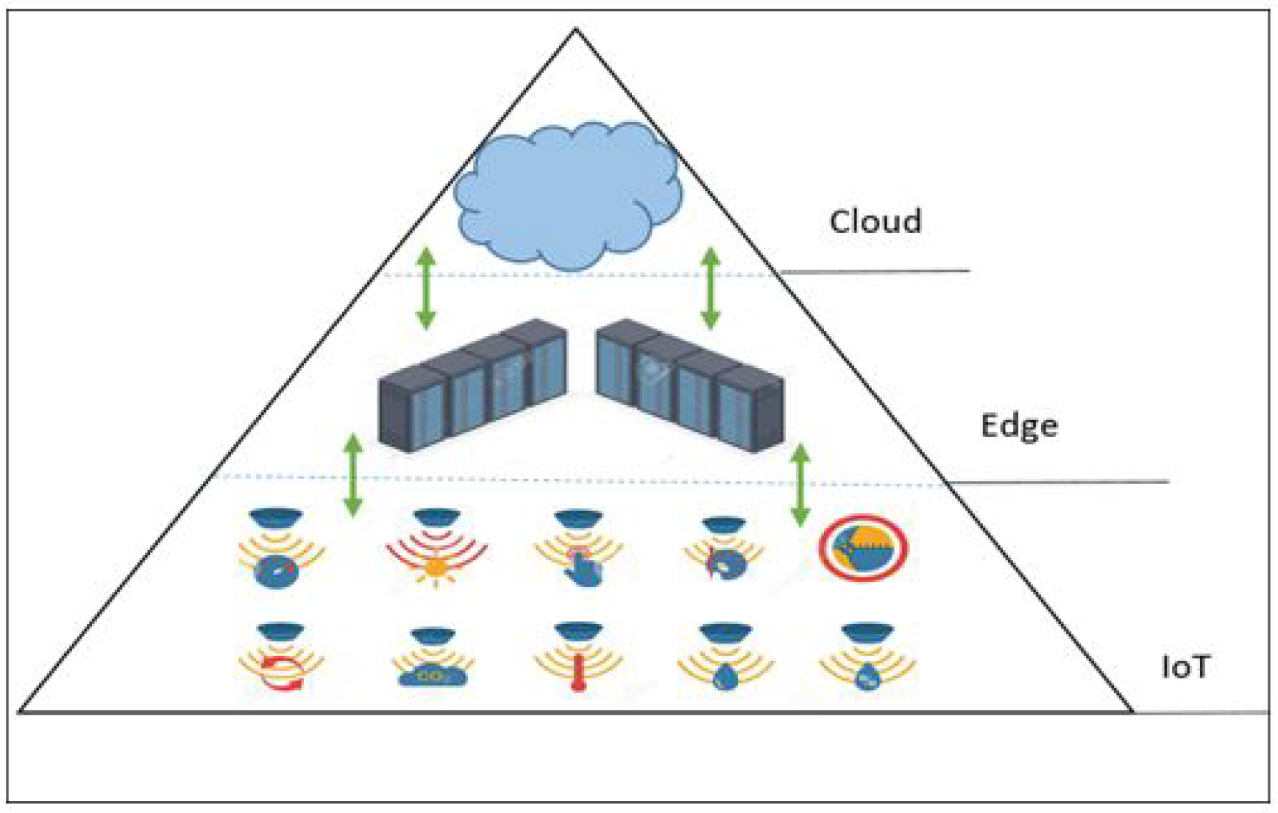
The widespread use of Internet of Things and robust cloud services has contributed to the demand for edge computing, in which data processing takes place in part at the network edge rather than entirely in the cloud [13]. Edge computing helps to solve issues such as bandwidth costs, latency, power consumption of mobile devices, security and privacy. Edge computing uses small data centres on the network’s edge to deliver distributed computing services and it acts as a middle interface between a cloud server and IoT devices/sensors [14,15]. In edge computing, the cloud takes data from the collected databases, as it has historically done, as well as from sensing devices and smartphones. The devices serve as both data consumers and data generators. As a result, queries between end devices and the cloud can be bidirectional, rather than merely from end devices to the cloud. To minimise traffic from devices to the cloud, nodes at the network edge perform a variety of computational functions, including data processing, device management, caching, and privacy protection (see Figure 1). Edge computing, in contrast to mobile cloud computing, allows for real-time data analytics while maintaining privacy, expands network capabilities, and avoids congestion in backbone networks and the internet core [16,17].

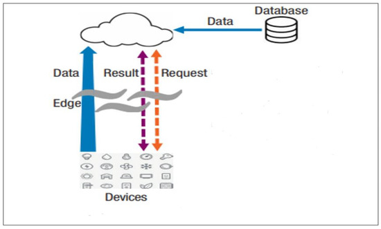
Figure 1. Data analytics using edge computing.

This paper investigates the use of edge computing for data analytics by integrating the edge with cloud computing to deliver deep learning applications. Four different scenarios have been used to identify the optimal framework for edge-cloud computing framework to monitor water quality. The organisation of this paper is as follows: Section 2 describes the benefit of applying edge intelligence in IoT, and Section 3 reviews the most relevant research on using edge-cloud computing for providing real-time applications. Section 4 describes the proposed framework and how it is investigated in more detail, and Section 5 presents the numerical results and discussion of these results. Finally, Section 6 concludes the work and shows the future work.

2. Edge Intelligent with IoT

This section introduces the architecture of edge intelligence in IoT and presents deep learning at the edge for different IoT applications.

2.1. Cloud-Edge Intelligent Architecture

Cloud is a centralised infrastructure system that stores data, executes business models, and performs data analytics activities at a long distance away from data sources and end-users [18]. However, with large-scale traffic and a proliferation of connected devices, it is neither feasible nor feasible to transmit all data to the cloud for processing. Edge computing has arisen as a means of addressing these issues by shifting processing to the network’s and data sources’ edges [19,20]. Edge computing and fog computing share similar characteristics. Sometimes, the terms “fog” and “edge” are commonly used to describe the same thing [21]; but the difference is that edge computing is primarily focused on nodes that are closer to IoT devices, while fog computing may encompass any resource that is situated anywhere between the end device and cloud [22]. In this work, we use the word “edge” to refer to compute nodes that are near the water network edge, such as edge servers [23]. Even though edge computing reduces traffic, the computer resources accessible on the edge do not have the same capabilities as those available in the cloud. As a result, computationally intensive processes like machine learning are not well suited to edge devices. However, the edge can enhance cloud computing by performing a portion of the computation, lowering network traffic and latency [24].

As illustrated in Figure 2, the edge-cloud learning framework is made up of three primary components: end-user devices, edge learning servers, and remote cloud deep learning clusters [25]. End-user devices, such as mobile phones, cameras, and internet-of-things sensors, send data to the edge server, which can be noisy and highly redundant [26]. Edge computing servers collect enormous amounts of raw data from end-users and utilize pre-processing and basic learning algorithms to filter out the noise and extract significant features from the raw data. Deep learning tasks, such as convolutional neural networks (CNN) and artificial neural networks (ANN), are carried out by the deep learning cluster (cloud), which is outfitted with scalable and robust GPU resources [27].

Figure 2. Standard edge-cloud architecture.

2.2. Deep Learning in Edge Computing

Typically, IoT devices generate significant amounts of data and send it to the cloud for processing. These data include multimedia information like photos, sounds, videos, and structured data like vibration, temperature, and humidity. There are numerous developed solutions for analysing structured data and then operating IoT devices autonomously [28]. Deep learning has been successful in many fields, including multiple visual tasks, speech recognition, natural language processing and industrial applications [29], this is because of its capacity to learn complicated models, and diversity of architectures [30]. A deep learning network is often composed of numerous layers. These layers will process the input data. Each layer processes the previous layer’s intermediate features and then generates new features. Finally, the extracted features generated by the final deep learning network layer will be recognised as the output by a classifier. Deep learning networks consider the layers closest to the input data to be lower levels, while the others are higher layers [28,31].

In this work, we have used an MLP model to detect and classify water contaminant levels for data that include water quality parameters. The developed model contains several layers that are completely connected. The model was trained using time series data for more than 50,000 samples. The MLP model was used to classify the data into five different classes representing the various levels of water contamination. Deep learning increases prediction accuracy for IoT services by extracting features through numerous layers rather than traditional complex pre-processing. However, with increased accuracy, communication performance will be the bottleneck. The amount of data needed to train deep-learning models is huge. Such a large volume of network traffic can cause various changes to the network in terms of increasing transmission delay, reducing the packet delivery ratio, increasing energy consumption due to high transmission rate, and may pose security risks; therefore, typical cloud-based solutions for deep learning approaches on IoT may not be ideal [32].

As illustrated in Figure 3, we present an edge computing topology for IoT deep learning applications. The structure is composed of two layers and also a normal edge computing structure. Edge servers are placed at the edge to process gathered data and the cloud server is used to train the deep learning network [33]. Applying deep learning entirely at the edge will reduce network traffic. However, the capacity of edge servers is limited compared to cloud servers. It is impossible to process infinite tasks in edge servers. Dedicating the entire work of deep learning to the edge will bring additional computing overhead to the servers. Therefore, we can only deploy part of the deep learning network into edge servers. The issue is deciding how to partition each deep learning network.

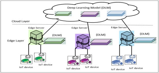
Figure 3. Deep learning in edge computing.

3. Related Work

Edge computing became more popular, particularly for applications with rapid response times and restricted bandwidth, since it places computing near data sources. Edge computing can be applied in different applications including smart cities, smart vehicles, smart traffic lights, and smart grids. These applications quickly integrate edge computing into their platforms, greatly increasing response time and saving network resources.

3.1. State-of-Art of Edge-Cloud Computing

Authors in [11] validated edge computing’s efficiency and resourcefulness. Edge systems are carefully surveyed, and a comparative cloud computing system research is presented. The results demonstrate that edge computing systems perform better than cloud computing systems after studying various network aspects of the system. In comparison to cloud computing standards, the current edge computing and fog computing standards provide stable and enhanced quality of service for IoT applications. Cao et al. in [34] examined a joint communication and computation user collaboration for mobile edge computing to enhance the power consumption for mobile edge computing (MEC). Consider a basic three-node MEC framework consisting of a helper node, an access point node, and a user node connected to an MEC server for demonstration purposes. A nearby helper node is enabled to contribute its computation and communication resources to increase the user’s computing performance. Numerical findings show the value of the collaboration in computing and communication offered by the users. Another study by Wang et al. [35] performed a full review of edge computer state-of-art research initiatives. This model integrates computing, caching, and communication resources. The edge computing is initially outlined, including description, design, and benefits. A complete examination of computing, caching and communication concerns is then provided at the network’s edge. The proposed framework architecture is composed of mobile edge, fog computing, and cloud. Mao et al. [36] provided a summary of significant advances in research for edge computing. Modelling methodologies for key edge computing (EC) components, such as computing tasks, communications, mobile computing, and the EC servers, were initially summarised. Models of essential elements of EC systems such as computation tasks, communications, and the computation of mobile devices and MEC servers were initially summarised. This facilitates characterising the latency and energy performance of EC systems. A research perspective is also presented, which contains a set of prospective MEC research guidelines. Finally, they discussed current industry standardisation initiatives, as well as numerous common application scenarios. The surveys addressed [11,34,36] highlight the potential of edge computing in data analytics and the relevance of edge computing in IoT for dealing with the number of linked devices that is rapidly increasing. As our work contributes to the use of edge computing for data analytics by merging edge and cloud computing for the delivery of deep learning applications, different applications for both IoT and edge cloud computing are reviewed below.

3.2. IoT Applications Based on Edge-Cloud Framework

One of the most often mentioned use cases and applications of edge computing is smart cities. Mohamed et al. [37] described how the service-oriented middleware (SOM) approach might benefit from resolving the issues associated with designing and managing smart city services utilising cloud and fog computing. They proposed SmartCityWare as a SOM for the complete coordination and usage of fog and cloud computing. The proposed framework isolates components and services used in smart city applications and makes them available as services via the service-oriented approach. This improves integration and enables the flexible incorporation and use of the many services required in a smart city application. Another study by Tang et al. [38] provided a multi-tier fog computing system for extensive data analytics in smart cities. Because of the inherent geo-distribution of massive data collected by enormous sensors, they disseminate smart at the edge of a tiered fog computing system. To maintain the safety of essential infrastructure components, computing nodes at each tier conduct latency-sensitive applications and offer rapid controller loops. Using smart pipeline monitoring as an example, a four-layer fog-based computing paradigm is presented to showcase the usefulness and feasibility of the system’s potential city-wide implementation.

Wang et al. [39] created a three-layer conceptual framework, dividing the city into zones for dispersed management. The fog and cloud layers offer potential computing abilities and resources for message processing without adding network expenses. According to queueing theory, model stationary and moving vehicle-based fog nodes predict the average reply time depending on their processing abilities. They conclude that moving fog nodes of vehicle-based may be seen as servers with queue theory M/M/1. To show the efficiency of the proposed framework, a performance assessment based on a real-world taxi path dataset is presented. In terms of average system response time and processing resources required, the proposed framework outperforms the competition. He et al. [40] proposed multi-tier fog for smart city applications with a large-scale data analysis service. The multi-layer fog is made up of devoted fogs and ad-hoc fogs, each having adaptable and dedicated computing resources. The developed novel fog computing framework, which includes distinct functional modules, can reduce the potential issues of a specialised computing platform and delayed reply in cloud computing. The results of experiments show that the analytical services are efficient across multitier fogs, and the proposed QoS systems are effective. In terms of job blocking likelihood and service utilities, fogs may significantly increase smart city analytical services than cloud models.

Other applications have used the edge-cloud framework for data analysis, Darwish and Bakar [41] proposed a new real-time intelligent transportation system (ITS) significant data analysis framework on the Internet of Vehicles (IoV) environment. The architecture presented fuses three dimensions: intelligent computing real-time extensive data analysis, intelligent computing, and IoV dimension, i.e., fog and cloud computing. This study also provides an exhaustive overview of the IoV setup lambda real-time large data analysis architecture, ITS big data characteristics, and various smart computing technologies. Sittón-Candanedo et al. [42] proposed an energy-efficient system using an edge-IoT framework and a social computing architecture inside a public building scenario. The system is assessed in a public building, and the findings show the remarkable advantages that edge computing brings to energy-saving circumstances and the framework. These advantages encompassed lowering the IoT-Edge data transmission into the cloud and lowering cloud, computer and networking expenses. The result of this work shows that systems with less computing capacity, consumption and hardware expenses may be deployed in a much more cost-effective manner by dividing computation loads from the cloud into the edge. Thakur et al. [43] presented a water conservation edge computing framework by employing easy computing methods. The proposed work helps decision-makers raise people’s awareness of water efficiency in a scientifically easy method. Based on numerous parameters such as the number of people, average family income, the profession of the members, and previous water needs, the proposed model leverages edge computing at the home nodes of the network to estimate the actual consumption of a specific home in real-time. Results reveal that the proposed approach operates better in a self-synthesised dataset than in other similar networks. The approach framework converges effectively and provides greater precision in spatial and temporal terms.

There are also other applications on health care and video streaming. Rahmani et al. [44] provided a fog-based computing-based framework that presents an implementation of an Internet of Things health monitoring system as a proof of concept. The proposed framework improves, for example, energy economy, performance, reliability, interoperability, and other diverse properties of IoT architecture utilised in health applications. A fog computing-based health IoT system and its services are described in more detail in the proposed framework, which is conducted from a variety of viewpoints. A medical case study named early alert cases to monitor patients suffering from acute diseases was applied to the fog-assisted system. All data flow operations from the data collection at sensor nodes to the cloud and end-users are part of our whole system demonstration. Sheltami et al. [15] proposed a framework for mobile users to employ fog computing as a content delivery system. The fog nodes are distributed close to mobile users. The users request the fog servers and answer each request, whether they are downloaded from the fog server or from the cloud if the request is just initialised. The findings show that fog computing gives minimal response time compared to the cloud. The studies also examine mobile users’ power consumption in different modes.

3.3. Edge Computing for AI

All the studies reviewed previously in this section used edge-cloud computing but for the non-machine learning task. The edge processing needs to accommodate the final machine learning computation for machine learning activities while decreasing the required network bandwidth and traffic [45]. Our work focused on using edge-cloud computing for machine and deep learning applications. Hence, it is essential to review a few works in this category.

Khelifi et al. [46] addressed the mapping of deep learning and information-centric networks (ICN) with IoT at edge computing and their potential benefits. They also introduced an effective component that enhances IoT by making the edge more intelligent. As a result, a convolutional neural network (CNN) model can be employed in the IoT area to use data from a complicated environment reliably. Furthermore, reinforcement learning (RL) and recurrent neural networks (RNN) have recently been integrated into IoT, which can be utilised to account for data multimodality in real-time applications. Ran et al. [47] proposed a distributed framework, DeepDecision, that links computationally weak devices (assuming that they’re smartphones) to more robust back-end devices that let deep learning in choosing local or remote execution. Any device that delivers the required computing power can be worked as the back-end helper. They are especially interested in running a CNN developed for recognising objects in real-time for augmented reality applications. Another work by Zhao et al. [48] presented a unique distributed deep learning framework (DDL). The DDL enables mobile edge nodes in the network to cooperate and interchange information in order to decrease the error of content demand estimation without compromising mobile users’ private information. They demonstrated through simulation findings that their proposed approach can improve accuracy by lowering the root mean squared error (RMSE) by up to 33.7 percent and minimising service latency by 47.4 percent compared to other machine learning techniques.

All the papers reviewed in this section show that cloud computing is the computing platform that is currently being used to analyze and monitor the quality of water. Therefore, we decided to take advantage of distributed computing and apply edge computing to monitor water quality and make real-time decisions.

4. System Model: Proposed Framework

In this work, we take a water distribution system as a case study to introduce our proposed intelligent edge-cloud framework to monitor drinking water quality. Figure 4 depicts the proposed distributed edge-cloud framework consisting of IoT devices and edge nodes equipped with edge server functionality and remote cloud. Compared to cloud servers, edge servers typically have more resources than IoT devices and are physically closer to them. In the IoT layer, water quality sensors are deployed in the WDS. This layer takes seven water quality indicators that are utilised to monitor the quality of the drinking water by using AI models, these features are chlorine (Cl), turbidity (TUR), PH, total organic carbon (TOC), temperature (TEMP), conductivity (COND), and pressure (PRES). To communicate edge servers and IoT devices, we used a communication technology suited for a short distance and lightweight IoT protocol (ZigBee). Using the same medium and protocol from both IoT devices and edge servers benefit in the following:

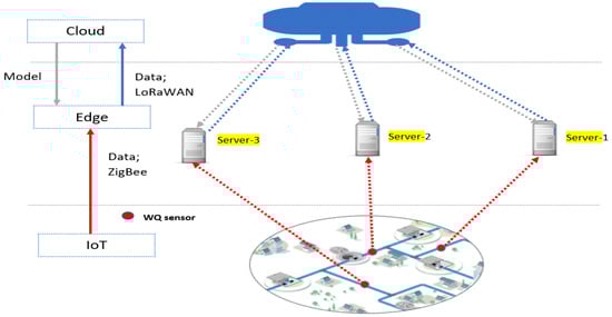
Figure 4. Proposed intelligent edge-cloud framework.

• Reduced design complexity due to the use of only one network stack and eliminating the requirement to convert packets from one format to another.
• Packet conversion is not required, which decreases energy consumption and latency.

However, the training phase of some machine learning algorithms, such as MLPs, puts a lot of pressure on edge servers’ computational capabilities and the backbone network’s communication resources, as training data must be obtained from sensors. Thus, the intelligent computational architecture must be altered. In this regard, we proposed an IoT intelligent computing architecture that consists of a two-tier smart data center, namely the edge layer and cloud layer. Edge and cloud computing work together to provide water quality sensors with near real-time computing through the edge layer and comprehensive and powerful computing through the cloud layer.

• Edge layer: It supports lightweight IoT intelligent computing services, while edge server computing services can be distinguished by computing application and service accuracy. This layer mainly works for the purpose of detecting water contaminants using deep learning models. The MLP model is trained and used for detection at the edge layer, as presented in scenario 1 explained below. The ensemble model is trained in the cloud and then used for detection at the edge layer, as illustrated in scenario 3. While edge servers act as a data forwarder to cloud computing, as explained in scenario 4.
• Cloud layer: It offers IoT users a strong and comprehensive computing solution at the cost of latency and connection overhead. It was used as long-term storage for data, as explained by Scenario 1. It has been used to train detection models using deep learning, as in scenarios 2 and 3. It was used to carry out all the tasks assigned to it to monitor water quality using deep learning models as in scenario 4.

To investigate the functionality of the proposed framework, four different scenarios will apply, whereby the functionality provided by both the edge and the cloud computing layers will be changed.

4.1. Scenario 1 (Fully Distributed)

In this scenario, training the MLP model and the detection apply at the edge layer. The framework initialises to work using an offline MLP model that is already pre-trained using historical data. The model keeps updated and trained at the edge using the real-time data that come from the sensors. The edge servers here conduct all functions train the model and use the model for detection, as shown in Figure 5.

Figure 5. Architecture for scenario 1.

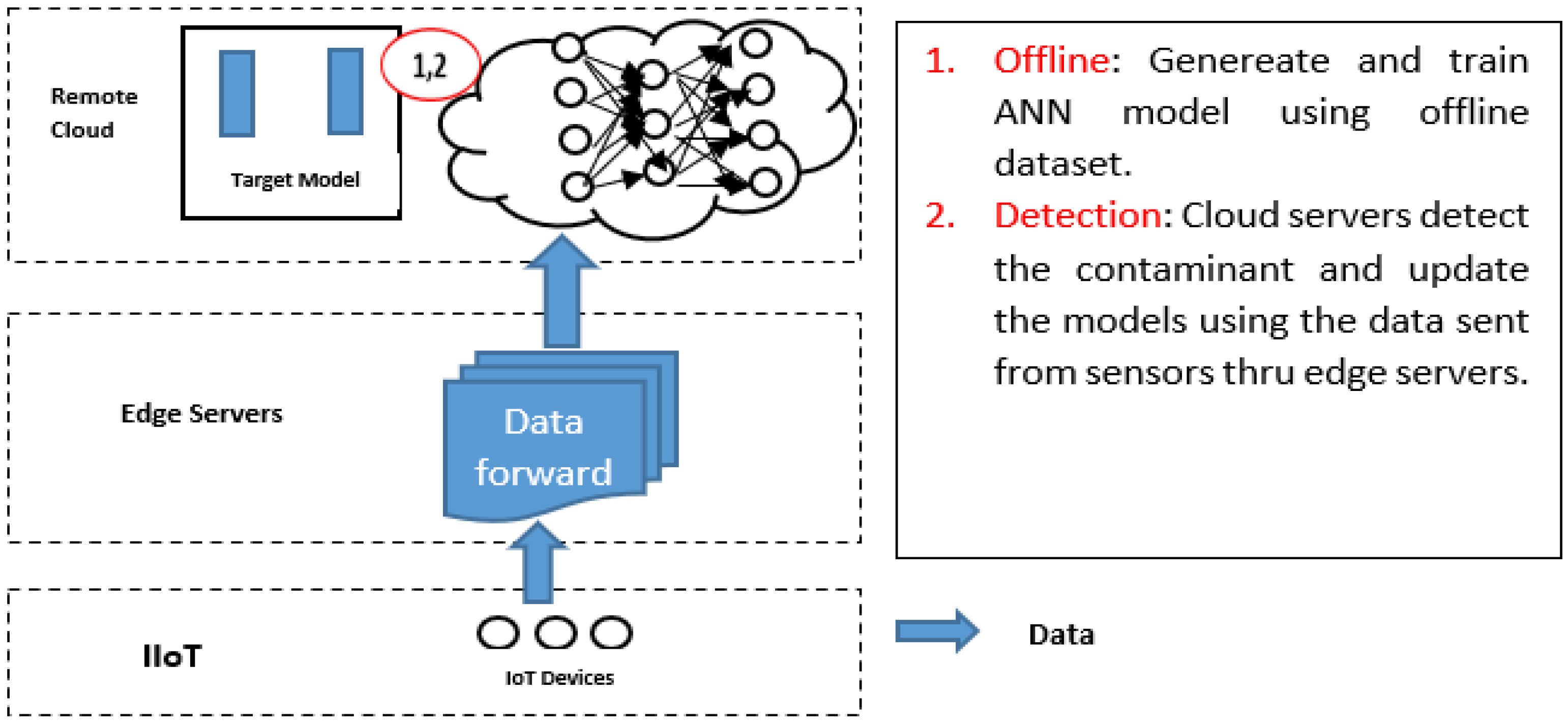
4.2. Scenario 2 (Train Mlp Model at Cloud and Detect at Edge)

The MLP model is trained in the cloud and sent down to the edge layer for detection. In this scenario, the edge servers have two functions:

• Continuously forward data to the cloud to continue the training.
• Use the trained MLP model downloaded from the cloud for detection as shown in Figure 6.
  

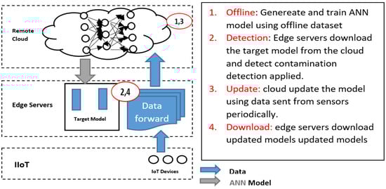  Figure 6. Architecture for scenario 2.

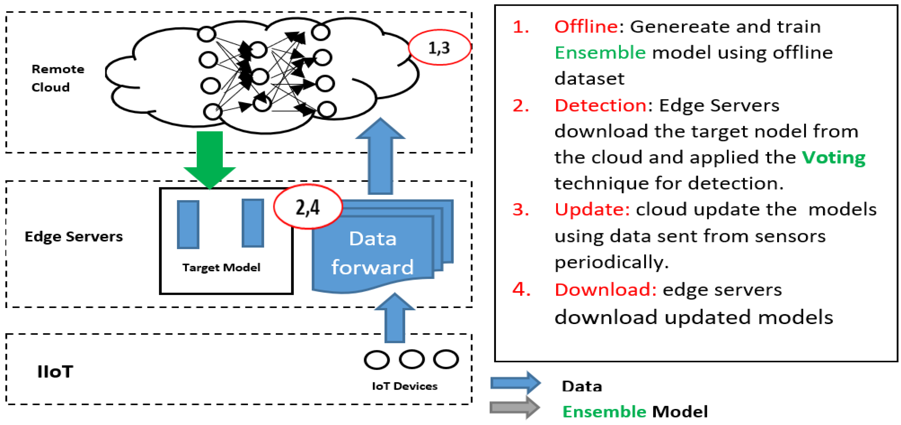
4.3. Scenario 3 (Train Ensemble Model at Cloud, and Detect at the Edge)

In this scenario, the third scenario aims to enhance the MLP model’s performance by applying ensemble learning in the cloud and sending the enhanced MLP model to the edge layer for detection. To take advantage of the high power resources at the cloud computing layer, ensemble learning (training) applies to the cloud. The ensemble uses different voting task models to select the suited model to apply at the edge (detection) as shown in Figure 7.

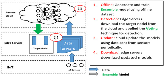
Figure 7. Architecture for scenario 3.

4.4. Scenario 4: (Fully Centralised)

Fourth scenario (fully centralised), in this scenario, all tasks apply at the cloud layer and edge servers work as data forwarders. All data need to be sent to the cloud in more detail, and the MLP model generated, trained, and used for detection at the cloud (See Figure 8).

Figure 8. Architecture for scenario 4.

5. Results and Discussion

5.1. Network Topology

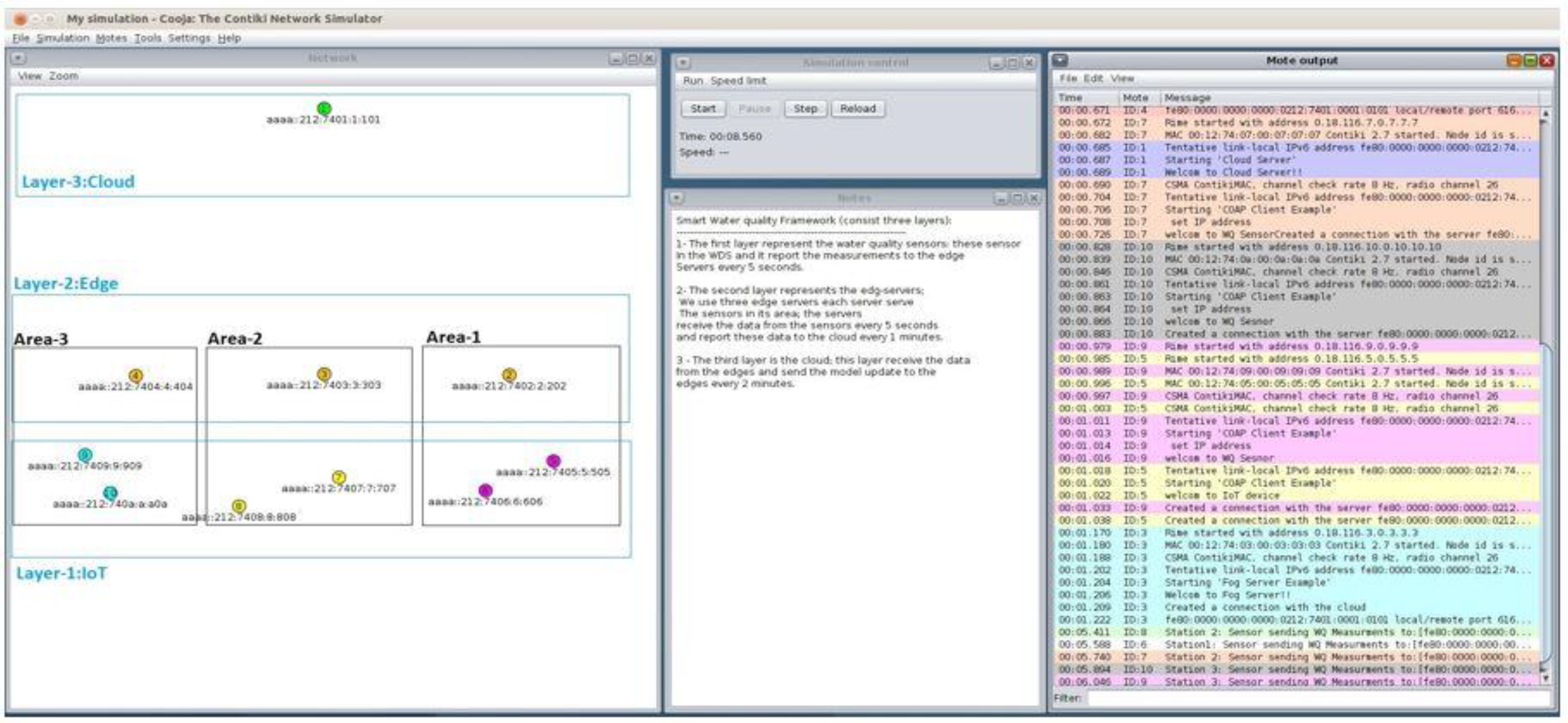
The proposed framework consists of three different layers: IoT in WDS, edge layer, and cloud layer as explained in the previous section. The network topology used to represent this framework is as follows. The case study (WDS) was divided into three different zones: Area-1 (B), Area-2 (C), and Area-3 (F) as shown in Figure 9. Each area contains a number of drinking water quality sensors, and these sensors were positioned in the area using optimisation method that was applied in the WDS [49]. A separate edge server is assigned for each area, and it is responsible for all water quality sensors located in its area. Water quality sensors need to establish a connection with edge servers, and edge servers establish communication with cloud servers. Another connection is also required, as cloud servers require establishing a connection with edge servers.

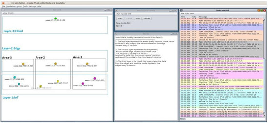
Figure 9. Network topology.

ContikiOS with CooJa simulator was used to implement the communication of our proposed framework. Contiki OS is an open-source operating system for resource-constrained hardware devices with low power and less memory [50]. It was developed mainly for Internet of Things applications. It also has many features, such as the communication module encompassing uIP and 6LowPAN [51]. uIP is, known as “micro IP”, has been designed to integrate a minimum set of components needed for TCP / IP stacks [52]. 6LowPAN is a growing technology that allows the use of IPv6 over IoT devices [53]. ContikiOS also has an extra function that supports the resource constraint hardware with the following features: small size, limited memory, lower power, low bandwidth, short-range, and communication using radio [54]. On the other hand, Cooja is a wireless sensor network emulator based on Java across layers, and it is distributed with Contiki OS. It simulates different levels from the physical to the application layer and enables the emulation of the hardware of a group of sensor nodes [55].

5.2. Experiment Setting

In order to develop the proposed framework presented in this work, we use data collected from three different zones in the case study as explained in the network topology. For that, edge servers are implemented using a Constrained Application Protocol (CoAP). CoAP is a constrained application protocol designed for IoT applications. Simplistically, CoAP is a machine-to-machine protocol built based on the request/response client-server paradigm and it is quite similar to HTTP [56]. It also supports the CoAP supports built-in discovery of services and resources. The main features of this protocol are: connectionless, lightweight, RESTful, and has a small 4-byte header. This protocol is used to manage the communication and data transfer between the sensors and edge servers on one side and the edge server and cloud servers on the other side. We have used two different communications technologies to establish the connection between the sensors with the edge servers and edge servers with the cloud server. ZigBee was used to offer the communication bridge between the edge and sensors as they are typically located closer to sensors in a ≤100 m range. LoRaWAN was used to provide the data from the edge to the cloud that were assumed to be apart from the edge servers with 10 km. More details of these techniques and parameters required are listed in Table 1.

Table 1. Communication technologies parameters.

Parameters	Values
Technology	ZigBee, LoRaWAN
Radio Medium	Unit Disk Graph Medium
Mote Type	TmoteSky
MAC Layer	CSMA/CA
Bandwidth (max)	250 Kbs, 50 Kbs
Payload	20 Kbps, 1.7 Kbps
Transmission Range	100 m

On the other hand, MLP was built using a sequential model with three layers: The input layer takes the seven water qualities: PH, TOC, temperature, conductivity, chlorine, and pressure. The activation function of this layer is linearly corrected. In this model, two hidden layers were used; the first hidden layer had 10 neurons, and the second hidden layer had 8 neurons; in order to activate both hidden layers, the rectified linear function was used. The output layer uses five classes have been used to represent the outcome (level of contamination) and Softmax used as an activation function. We used the “Adam” optimizer, as well as losses and accuracy for measurements. Summarised of all these parameters are presented in Table 2.

Table 2. Hyperparameters of the MLP model.

Hyperparameters	Values
Number of layers	3
Input layer	7 features as input; ReLU activation function
Hidden layer	2 hidden layers with 10 neurons for 1st and 8 neurons for 2nd. The activation function is relu
Output layer	5 classes; Softmax as activation function
Optimizer and losses	Adam, categorical_crossentropy and accuracy
Others	learning rate: 0.01; epochs: 200; batch size = 128

5.3. Numerical Results

In this section, the numerical results from all scenarios explained before will be presented. In addition, five metrics have been used to evaluate the performance of each scenario: latency, throughput, packet deliver ratio (PDR), power consumption, and model performance. Firstly, latency in a network refers to the time for data transmission across the network to its desired destination. One-way latency is measured in packet-based networks by sending a precisely timestamped packet across the network. The one-way delay is calculated by comparing the packet’s timestamp with the time of the receiving unit’s reference clock [57]. Secondly, the amount of data that may be transmitted from source to destination in a particular timeframe is referred to as network throughput [58]. Throughput capacity is often measured in bits per second, although it may also be measured in data (Kilobit or Megabit) per second. Throughput is calculated by dividing the data bits delivered to the destination by the delay time of communications data packets [59]. Moreover, (PDR) is defined as the ratio of packets transmitted to total packets sent from the source node to the destination node in a network. PDR describes the packet loss rate, which restricts the network’s throughput. The routing protocol’s performance improves as the delivery ratio rises. PDR is computed as:

$$PDR=\frac{P_{tr}}{P_s}\times 100$$

(1)

where $P_{tr}$ is the total packet received at the destination, $P_s$ is the number of packets sent from the source. For power consumption, we utilised the Contiki power tracer model, which reads the number of Ticks on a regular basis and computes the power consumption using the equation below [60].

$$Powr\left(mW\right)=\frac{Energst\times current\times voltge}{RTMER\times Runtime}$$

(2)

where $Energes{t}_{value}$ is the values in TICKS read from the simulator, $current$ and $voltage$ are the sensor values of current and voltage from the datasheet of the used sensors. $Runtime$ is the simulation time and $RTME{R}_{second}$ is the constant $value=$ 32,768 used to convert the values of the simulator from TICKS to seconds.

5.3.1. Results of Scenario 1

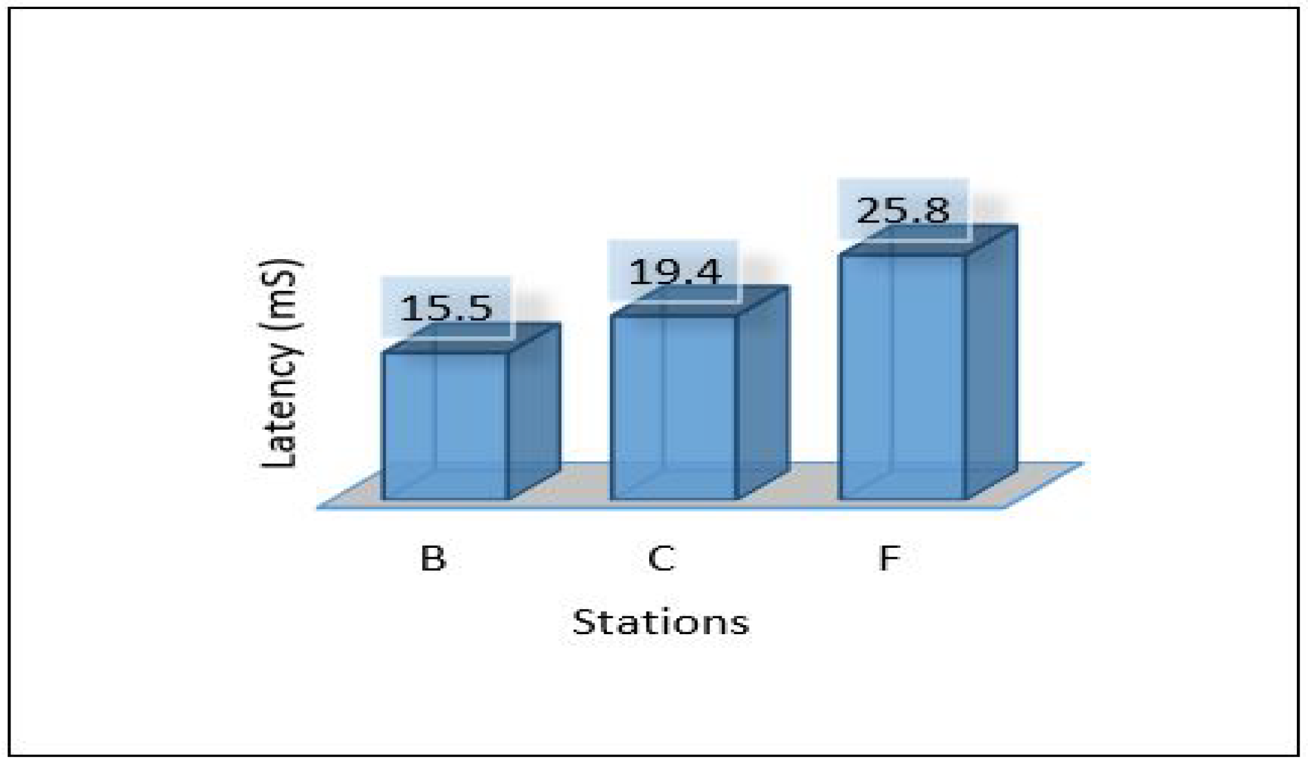
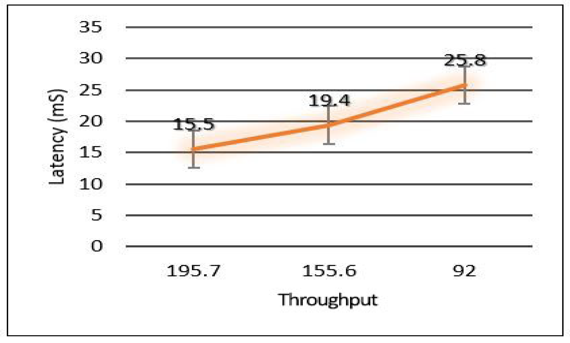
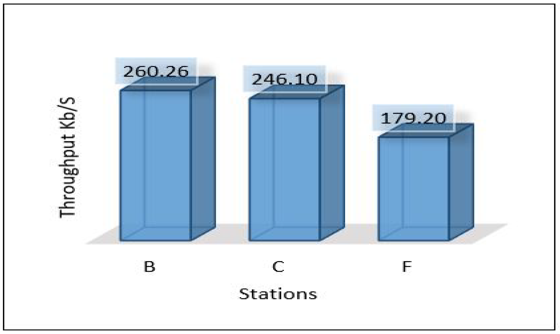
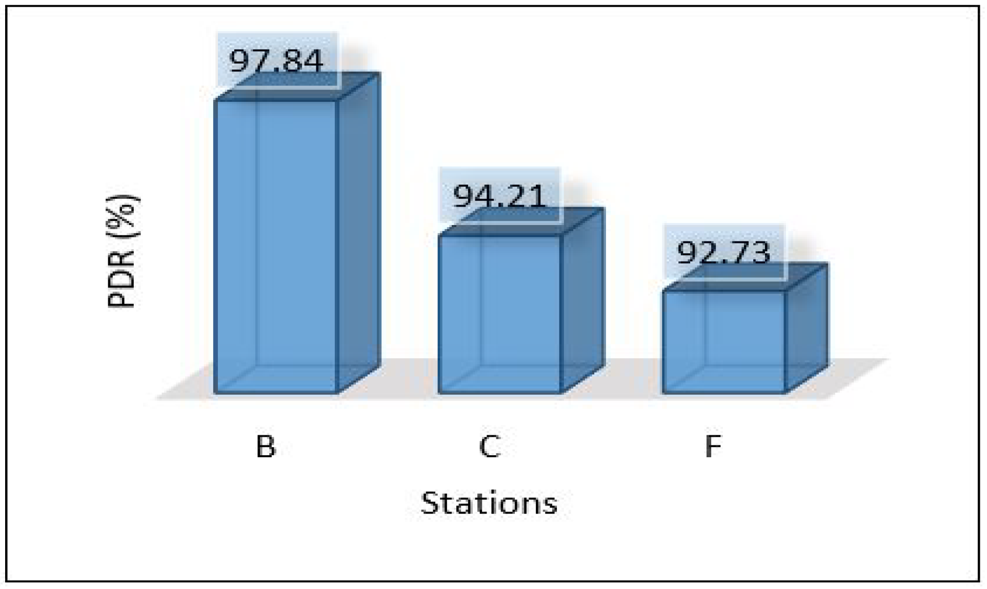
Since we used three different areas in our case study as explained in the network topology section. We need to evaluate the overall network performance by sending all the data from the lower layer (IoT-layer) to the upper layers (edge and cloud) in all three areas. The average latency for sending all data from the first layer to the edge server has been shown in Figure 10. We can notice the latency for the three areas is different due to the accessibility to the medium and the data size in which Area-1 recorded a low latency $15.5$ mS. In comparison, Area-3 recorded the height value of the average latency ($25.8$ mS). Figure 11 and Figure 12 show the average throughput used by each area during the transmission and the average packet delivery ratio (PDR) that offers the average success of packet delivery, respectively.

Figure 10. Latency of areas for scenario 1.

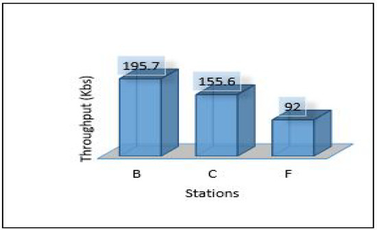
Figure 11. Throughput of areas for scenario 1.

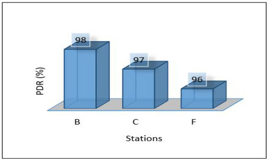
Figure 12. Packet delivery ratio for scenario 1.

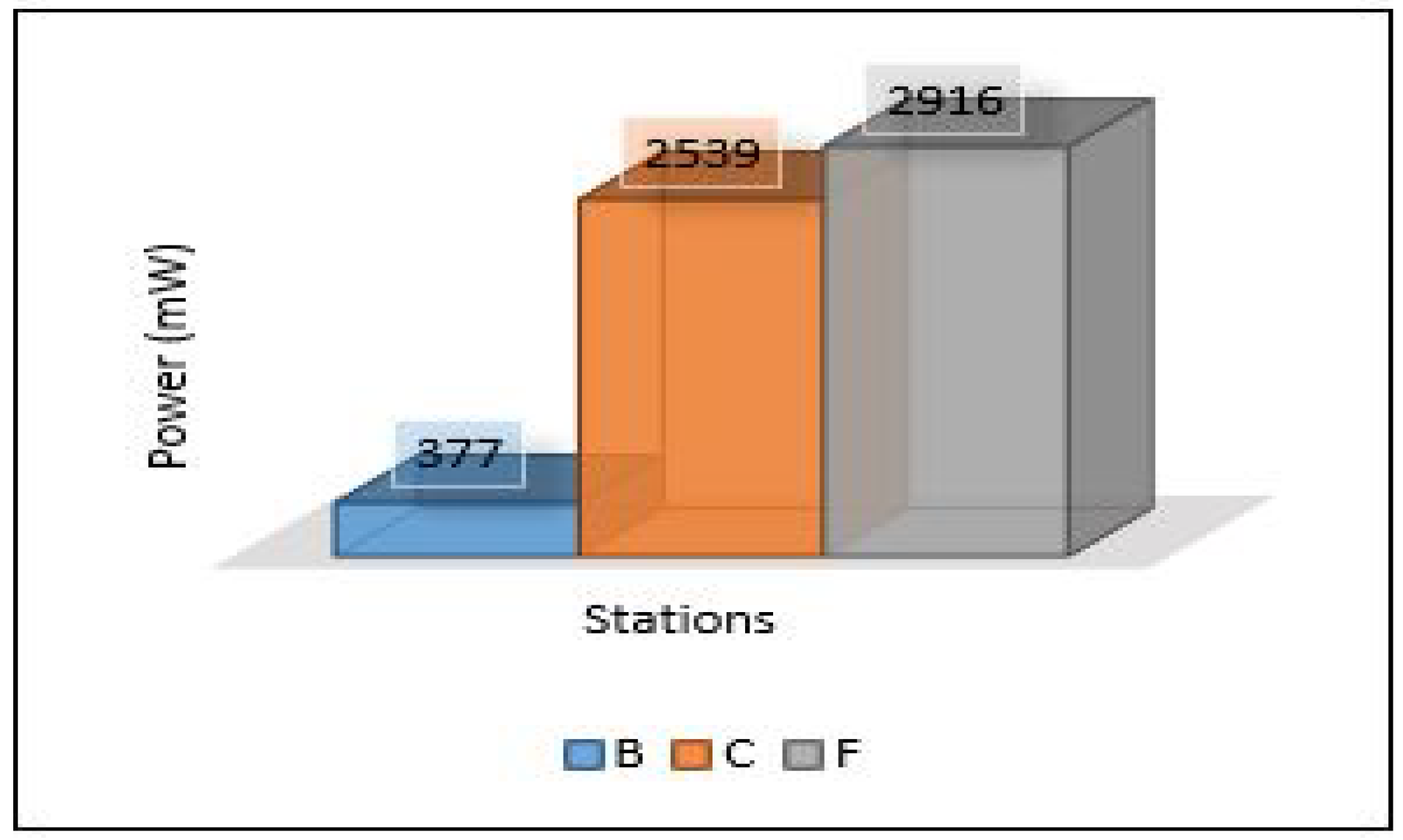
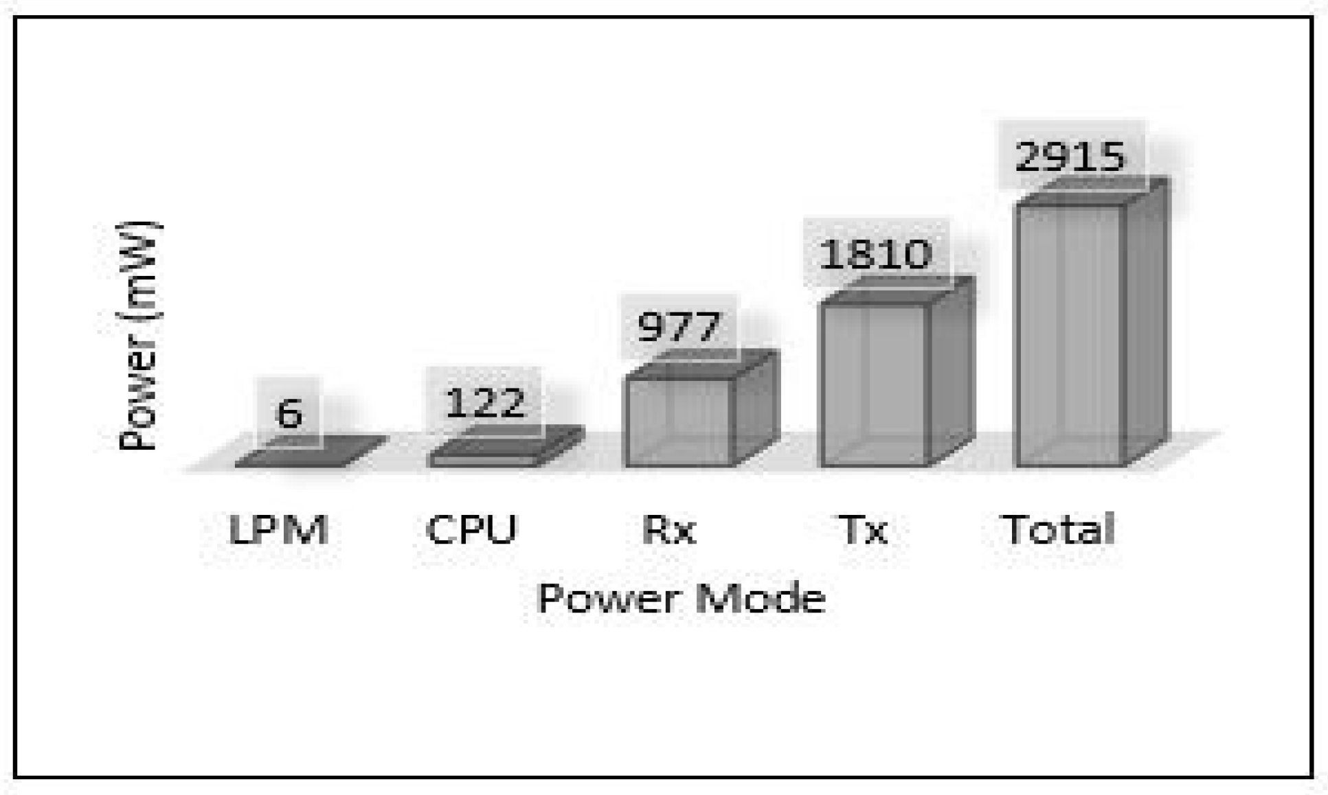
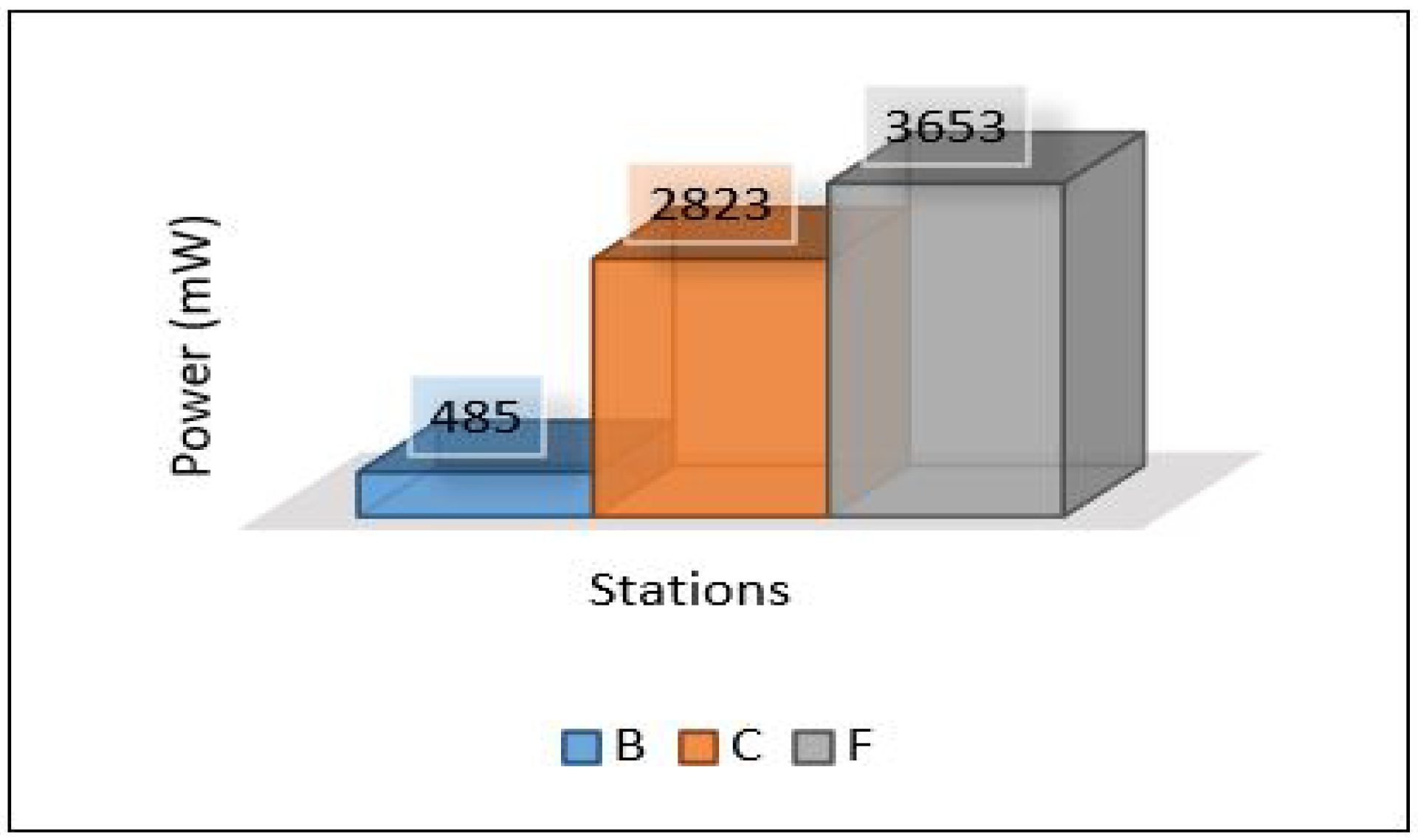
The relation between latency versus throughput is presented in Figure 13. We notice that throughput has a significant impact on both latency and PDR as increasing the throughput helps reduce the latency and increases the successful number of delivery packets. Considering power consumption as an essential metric for performance evaluation, we calculate the power consumption for edge servers and sensors. The amount of energy consumed for each device has been calculated based on four different models: low power mode (LPM), processing mode (CPU), receiving (Rx), and transmission (Tx). The total power consumption of sensors for each area (Area-1, Area-2, Area-3) is presented in Figure 14. Area-3 shows high power consumption because extensive data have been collected from that area, while Area-1 power looks small because it collected small data. The details of power consumption for Area-1, Area-2, and Area-3 including all modes are presented in Figure 15, Figure 16 and Figure 17, respectively.

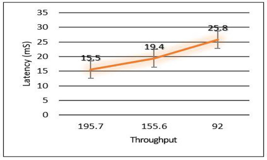
Figure 13. Relation of latency and throughput.

Figure 14. Power consumption for sensors.

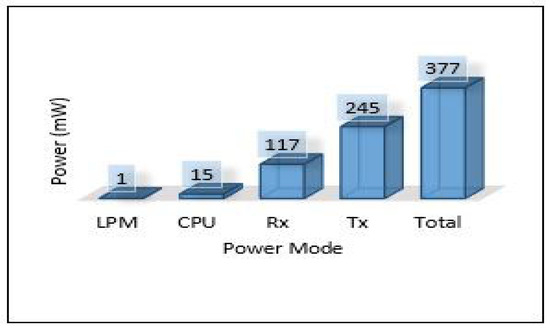
Figure 15. Power modes for sensor in Area-1.

Figure 16. Power modes for sensor in Area-2.

Figure 17. Power modes for sensor in Area-3.

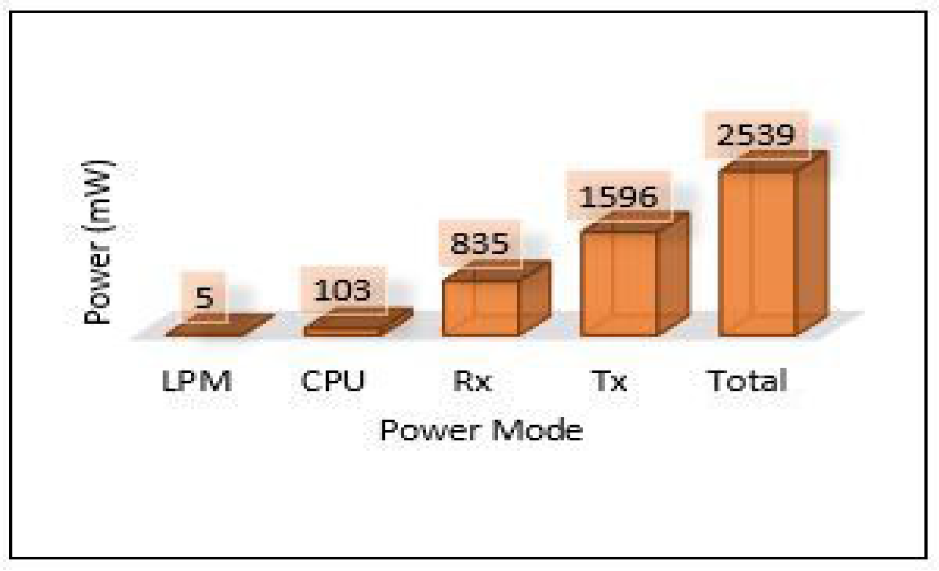
On the other hand, the total power consumption for edge servers has been calculated using the same mods used with sensors. Figure 18 presents the total power of all edge servers (Area-1, Area-2, and Area-3). We can notice that the edge servers used a huge amount of power in this scenario because all the tasks of training and detection for the MLP model have been applied at the edge layer. Most of this power was consumed by the processing mode (CPU) that performed all training and detection tasks, and the rest of the consumed power was distributed between the other modes, high for the receiving mode (Rx). Figure 19, Figure 20 and Figure 21 present the breakdown power consumption of all servers. These figures show in which mode the power consumption rate rises (LPM, CPU, Rx, Tx).

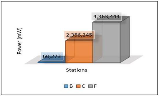
Figure 18. Power of servers for scenario 1.

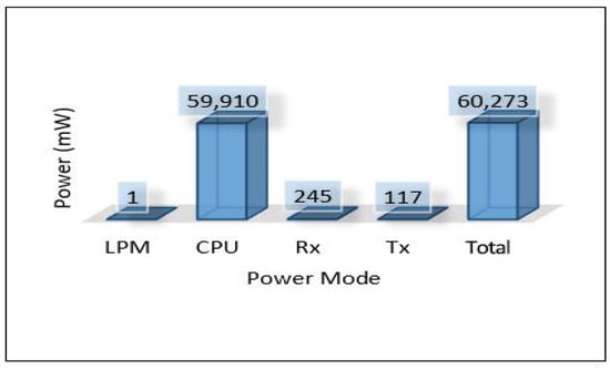
Figure 19. Power modes of edge server-1.

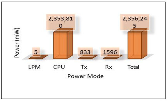
Figure 20. Power modes of edge server-2.

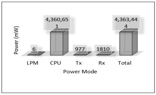
Figure 21. Power modes of edge server-3.

5.3.2. Results of Scenario 2

In this scenario, the MLP model trains and develops in the cloud and then needs to be sent back down to the edge, and we expect the latency to be higher than the latency of the previous scenario. Figure 22 depicts the total average latency that passed through three hops: sensor-edge, edge-cloud, cloud-edge (end-to-end) for the three areas. The result shows a high value at Area-3 and a low value at Area-1. The throughput used to send all data and models, and the PDR are presented in Figure 23 and Figure 24, respectively. Power consumption of the edge servers seems to be reduced compared to the previous scenario because the model’s training has been moved to the cloud, and the edge servers are used only for detection; see Figure 25 for the total average of power consumption for edge servers.

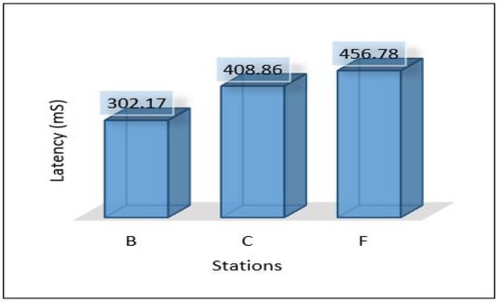
Figure 22. Latency of areas scenario 2.

Figure 23. Throughput of areas scenario 2.

Figure 24. PDR for areas scenario 2.

Figure 25. Power of servers scenario 2.

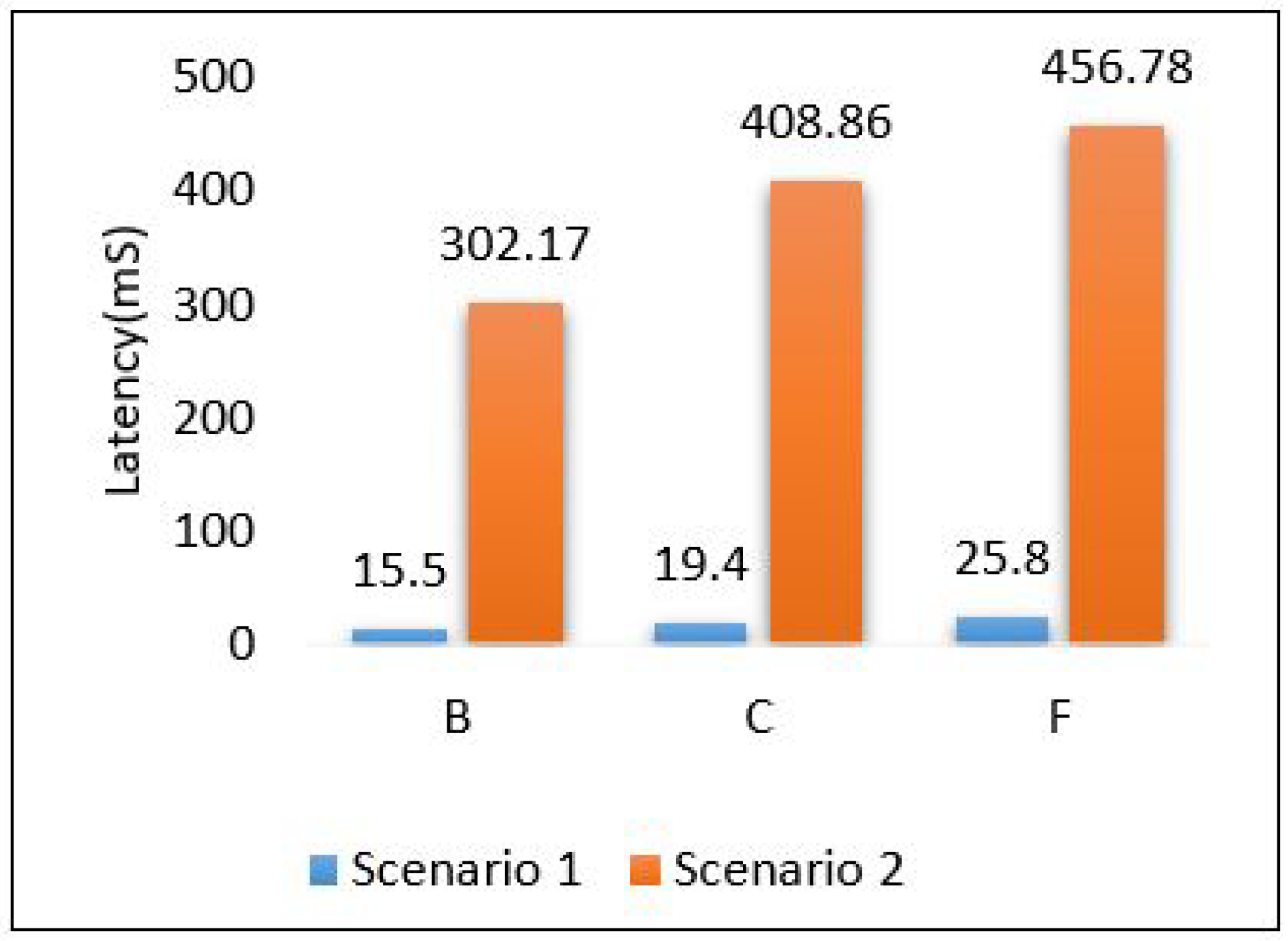
A simple comparison between scenario 1 and scenario 2 in terms of latency and power is presented in Figure 26 and Figure 27, respectively. The results show that scenario 1 outperforms scenario 2 in terms of latency while scenario 2 outperforms scenario 1 in terms of power, as scenario 1 consumes a huge amount of power. To sort the issue of power that appeared in scenario 2 and scenario 3 we will try to take advantage of cloud and edge by dividing the tasks between cloud and edge layers.

Figure 26. Comparison between scenarios 1 and 2: latency.

Figure 27. Comparison between scenario 1 and 2: power.

5.3.3. Results of Scenario 3

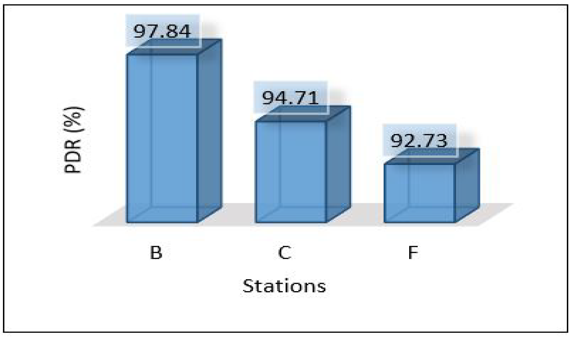
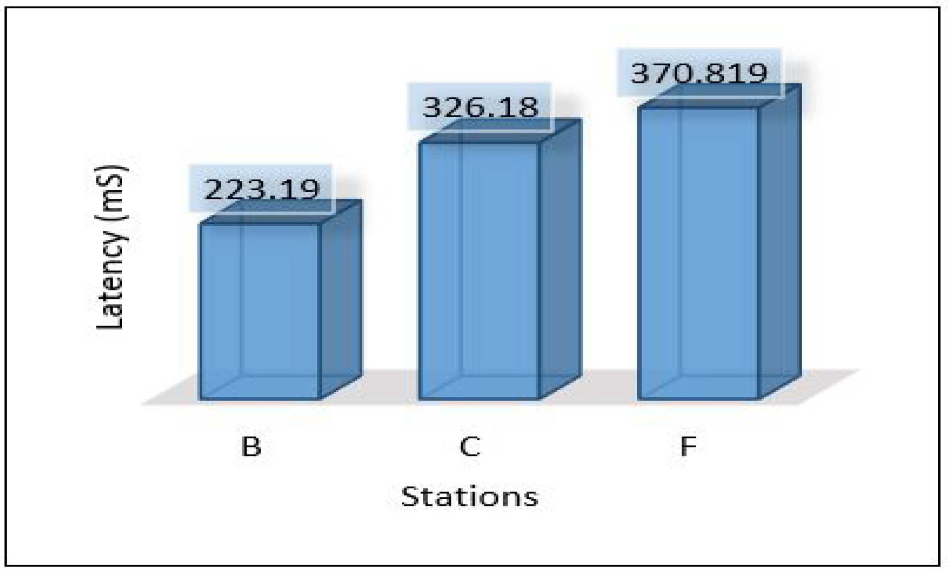
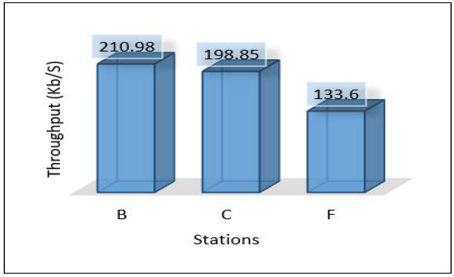
In this scenario, we applied ensemble learning to enhance the performance of the MLP model. The process of data analysis is divided between the cloud and edge servers. The cloud layer is used to train and develop the ensemble model and the edge layer uses the pertained model sent from the cloud for the detection. More precisely, edge servers are used to apply the voting technique for detection. Figure 28 shows the latency for all areas. In general, it seems that the latency is very high compared to previous scenarios while maintaining the same level between areas (Area-1, Area-2, and Area-3). Throughput and PDR seem to be the same with very little change compared to scenario 2 as shown in Figure 29 and Figure 30. The total average power consumption for the edge servers is presented in Figure 31.

Figure 28. Latency of areas scenario 3.

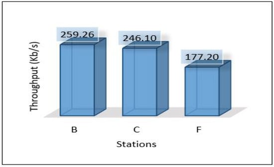
Figure 29. Throughput of areas scenario 3.

Figure 30. PDR of areas scenario 3.

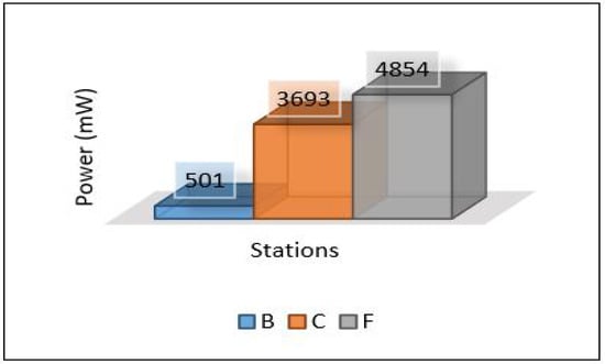
Figure 31. Power consumption of edge servers.

5.3.4. Results of Scenario 4

In this scenario, fully centralised is used. All data analysis tasks are performed in the cloud, so there is no need to send the model to the edge layer. This leads to reducing the latency compared to scenario 2 and scenario 3. Figure 32, Figure 33 and Figure 34 show the latency, throughput and PDR, respectively. This scenario has not calculated the power consumption for edge and cloud servers. Since the edge servers are used for a very light task as data forwarders, that will lead to very low power consumption that can be neglected, and the cloud assumes it is fully equipped with power all the time.

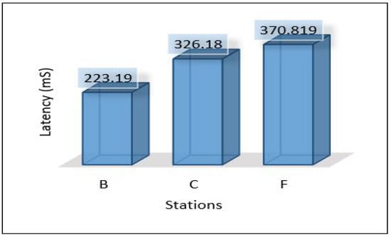
Figure 32. Latency for areas scenario 4.

Figure 33. Throughput for areas scenario 4.

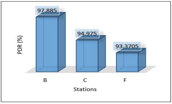
Figure 34. PDR for areas scenario 4.

5.4. Discussion

Through the above numerical experimental analysis, we can compare the performance metrics between all scenarios. For example, Figure 35 depicts the latency of all scenarios for each area, and we can conclude that scenario 1 outperforms all scenarios in terms of latency, as it has achieved the least delay in all areas with different data volumes. Figure 36 presents the throughput of all scenarios for the three areas; from the figure, it is clear that scenario 2 and scenario 3 require a very high throughput compared to the others. This is because sending data goes through 2-hops (edge, cloud) and sending the model from the cloud down to the edge. Scenario 1 shows that it requires a little throughput as it only needs to send data to one hop and does not require sending a model anywhere else. Scenario 4 plays a marginal role between scenario 1 and scenarios 2, and 3.

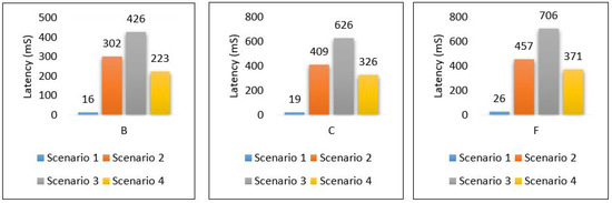
Figure 35. Latency for all scenarios based on each area.

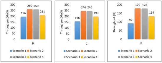
Figure 36. Throughput for all scenarios based on each area.

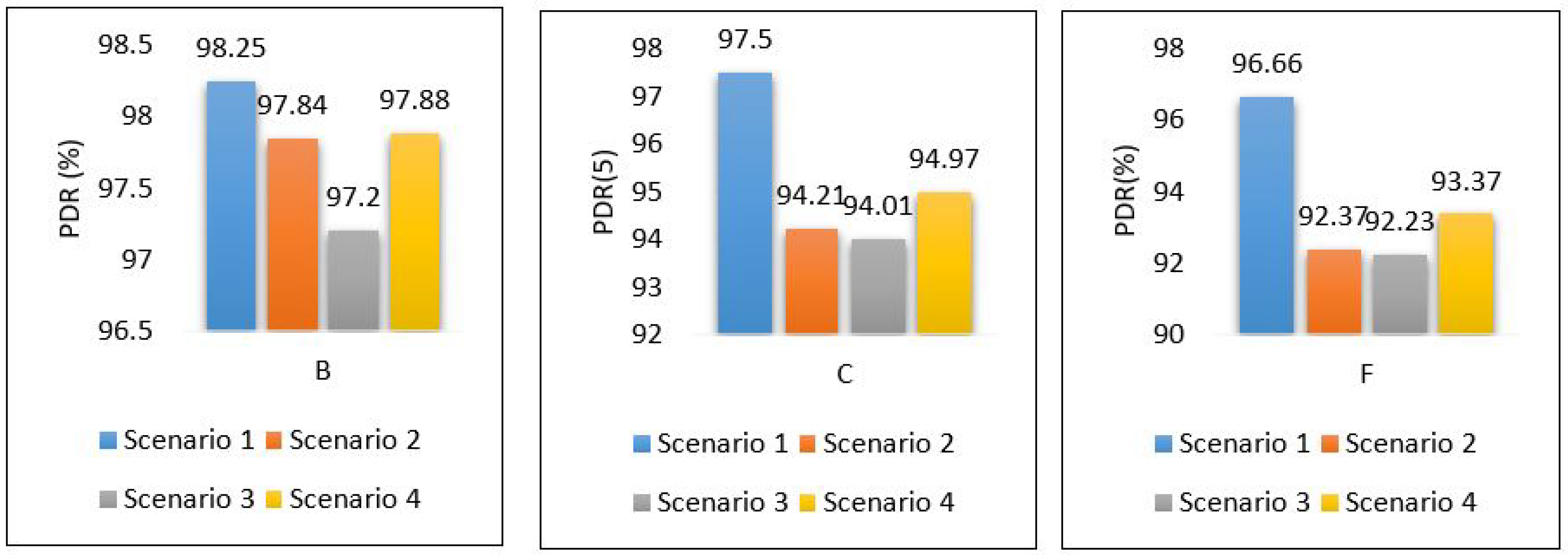
Figure 37 shows the PDR for each area separately. It shows that scenario 1 outer performs the others with a high percentage of successful packet delivery, and scenario 3 indicates the lowest rate of successful packet delivery. That’s because scenario 1 requires only one hop connection while scenario 3 requires three hop connections. This leads to an increase in the probability of packet loss.

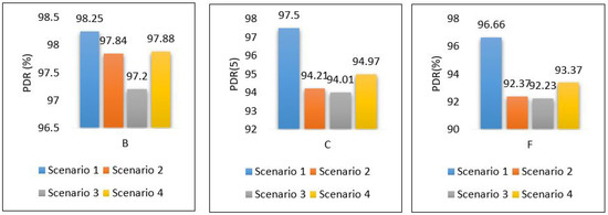
Figure 37. PDR for all scenarios based on each area.

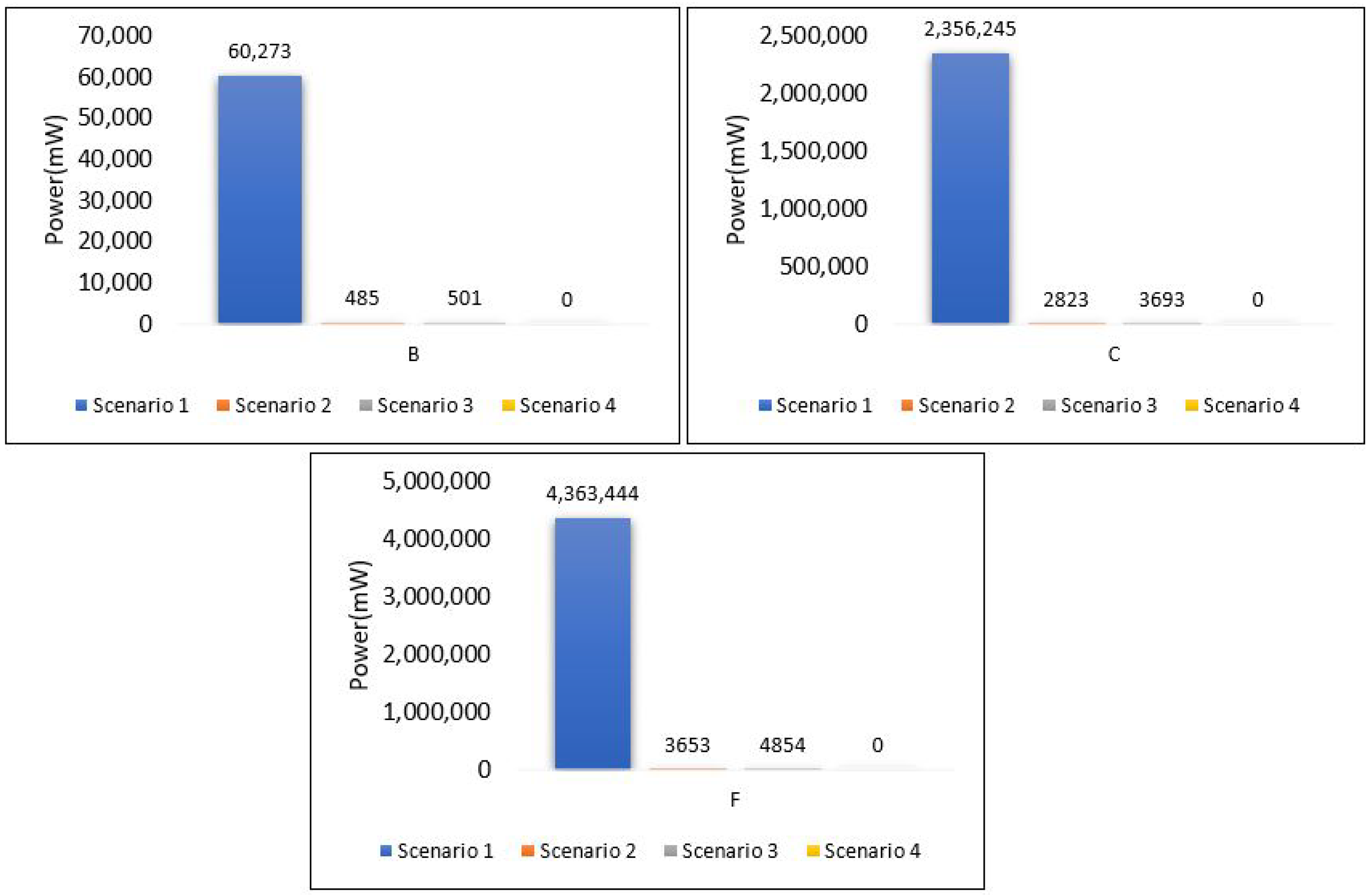
Power consumption for edge servers also was compared between all scenarios, as shown in Figure 38. The results here show the significant differences in power consumption between the first scenario and the others. Scenario 1 shows terrible power consumption compared to others because all the tasks required for training the model and for the contaminant detection process are performed at the edge layer. Looking at the power consumption in both the second and third scenarios, we find that the consumption is logically close to the increase in consumption in scenario 3 because the voting process required in ensemble learning is performed at the edge layer.

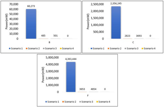
Figure 38. Power consumption of all scenarios based on each area.

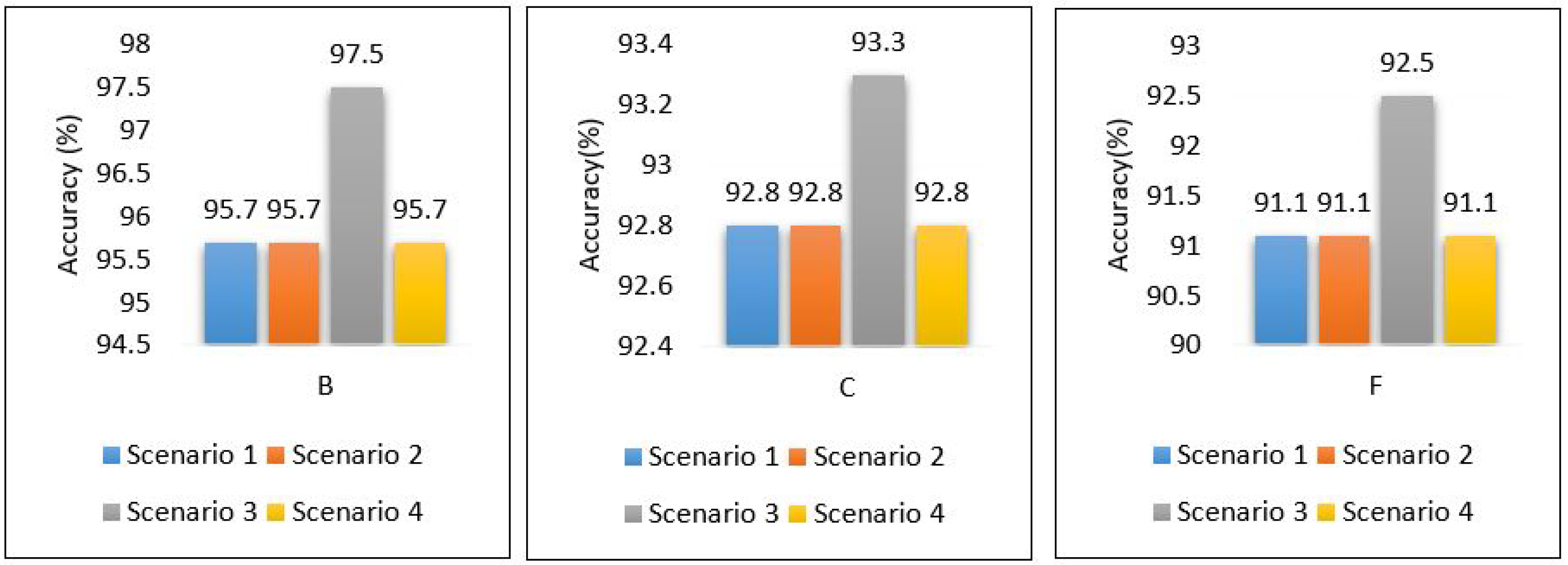
The performance of the MLP model is compared between all scenarios in Figure 39; the results show that the performance of the MLP model is stable and obtains the same accuracy regardless of the place in which it was implemented, whether in the cloud or at the edge. With the exception of scenario 3, it achieved the best performance, because we used ensemble learning, which helped improve the model’s performance without affecting the rest of the parameters, all energy consumption and delay.

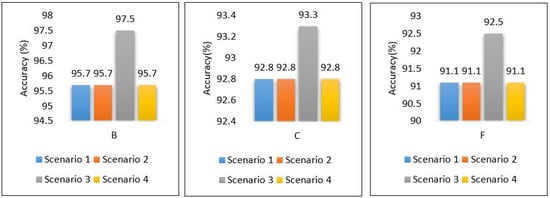
Figure 39. Performance accuracy of models for all scenarios based on each area.

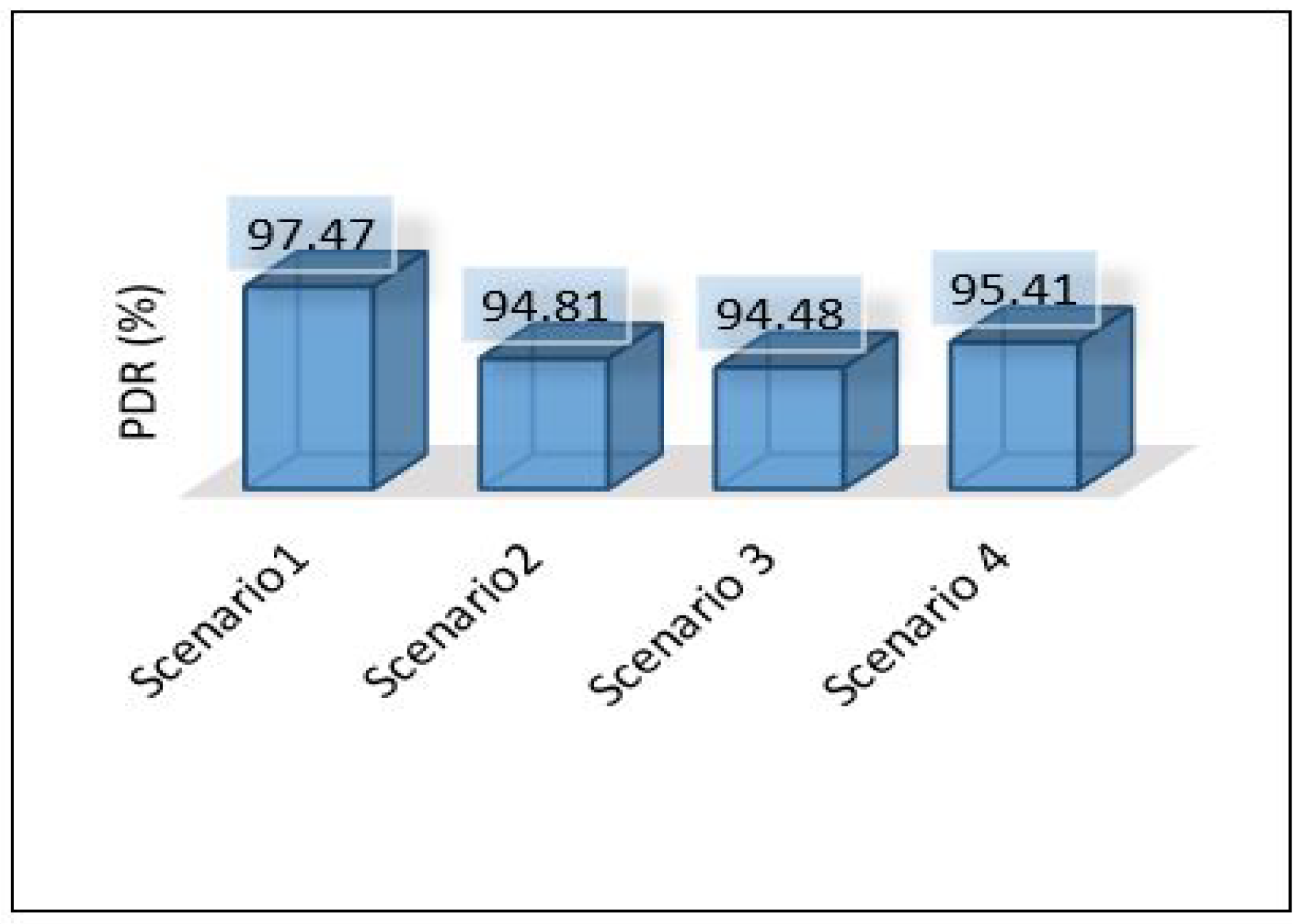
The overall performance of the framework presented for each metric is as follows: Figure 40 shows the overall latency for all scenarios. The result shows that scenario 1 is the best in terms of latency while scenario three is the worst one. Figure 41 shows the overall performance of the throughput, the results show that scenario 2 and scenario 3 required more throughput than others while scenario 1 required the lowest throughput. Figure 42, summarises the percentage of the successful packet received at the destination. The result shows that scenario 1 is the best while scenario 2 is the worst. Figure 43 shows the overall power consumption of the framework; it shows that scenario 1 is the worst with a very massive amount of power consumption, while scenario 3 is the best. Power scenario 4 is ignored as it performed totally in the cloud. Finally, the overall performance of the MLP model for classification is presented in Figure 44, the results depict that scenario 3 enhances the accuracy of the model while all other models recorded the same accuracy. In summary, taking all metrics into consideration, scenario 3 shows the optimal solution as it shows the best performance.

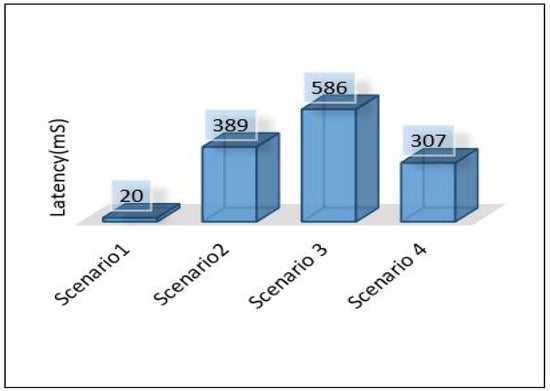
Figure 40. Overall latency of the framework.

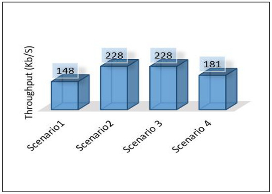
Figure 41. Overall thru of the framework.

Figure 42. Overall PDR of the framework.

Figure 43. Overall power of the framework.

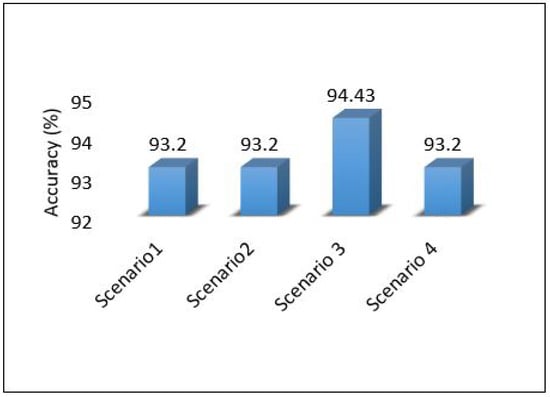
Figure 44. Overall performance of the classification models for the framework.

6. Conclusions

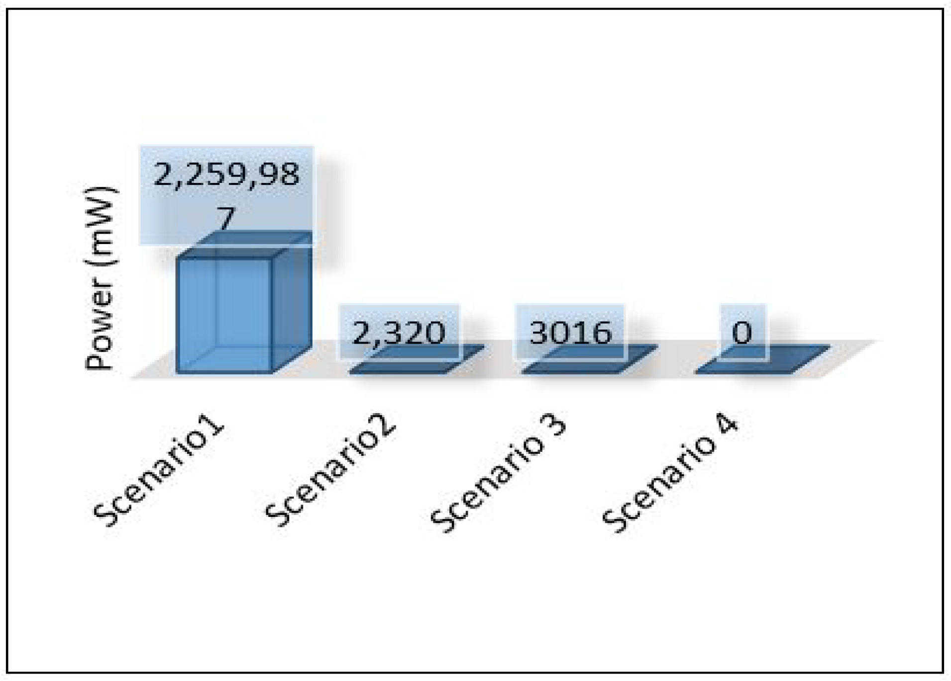
This paper proposes an intelligent computing architecture for water quality, based on collaboration between edge servers and remote clouds. A deep learning application aimed to provide real-time monitoring of water quality in WDS. Thus, the datasets from three different areas (Area-B, Area-C, and Area-F) in the WDS were used to develop the deep learning model and then evaluated the framework’s performance. The datasets include the main parameters used to indicate the quality of water such as chlorine, turbidity, Ph, TOC, conductivity, temperature, and pressure. Four different scenarios were applied in the proposed framework to investigate the ideal architecture for the used application. We have used Contiki with Cooja simulator to implement and simulate all these scenarios. We have used five different metrics to evaluate the performance of the proposed framework in all these scenarios. These metrics are latency, throughput, packet delivery ratio, power consumption, and deep learning model detection accuracy. The overall performance of the proposed work shows that scenario 1 outperforms the others in all stations (B, C, F) in terms of latency, throughput, and packet delivery ratio obtaining 20.33 mS, 148 Kb/s, 97.47%. On the other hand, scenario 1 shows the worst in terms of power consumption as it records a high value of 2,259,987 mW. In terms of model accuracy detection, Scenario 3 shows the best, and it records 94.43%.

References

- Xu, H.; Yu, W.; Griffith, D.; Golmie, N. A survey on industrial Internet of Things: A cyber-physical systems perspective. IEEE Access 2018, 6, 78238–78259. [Google Scholar] [CrossRef] [PubMed]
- Azzedin, F.; Ghaleb, M. Internet-of-Things and information fusion: Trust perspective survey. Sensors 2019, 19, 1929. [Google Scholar] [CrossRef] [PubMed]
- Krishnamoorthy, S.; Dua, A.; Gupta, S. Role of emerging technologies in future IoT-driven Healthcare 4.0 technologies: A survey, current challenges and future directions. J. Ambient. Intell. Humaniz. Comput. 2021, 14, 1–47. [Google Scholar] [CrossRef]
- Ur Rehman, M.H.; Yaqoob, I.; Salah, K.; Imran, M.; Jayaraman, P.P.; Perera, C. The role of big data analytics in industrial Internet of Things. Future Gener. Comput. Syst. 2019, 99, 247–259. [Google Scholar] [CrossRef]
- Liu, J.; Gui, H.; Ma, C. Digital twin system of thermal error control for a large-size gear profile grinder enabled by gated recurrent unit. J. Ambient. Intell. Humaniz. Comput. 2021, 14, 1–27. [Google Scholar] [CrossRef]
- Sun, W.; Liu, J.; Yue, Y. AI-enhanced offloading in edge computing: When machine learning meets industrial IoT. IEEE Netw. 2019, 33, 68–74. [Google Scholar] [CrossRef]
- Sipos, R.; Fradkin, D.; Moerchen, F.; Wang, Z. Log-based predictive maintenance. In Proceedings of the 20th ACM SIGKDD International Conference on Knowledge Discovery and Data Mining, New York, NY, USA, 24–27 August 2014; pp. 1867–1876. [Google Scholar]
- Shah, P.; Jain, A.K.; Mishra, T.; Mathur, G. IoT-Based Big Data Storage Systems in Cloud Computing. In Proceedings of the Second International Conference on Smart Energy and Communication, Bilaspur, India, 19–22 December 2021; pp. 323–333. [Google Scholar]
- Liu, W.; Huang, G.; Zheng, A.; Liu, J. Research on the optimization of IIoT data processing latency. Comput. Commun. 2020, 151, 290–298. [Google Scholar] [CrossRef]
- Shu, Y.; Zhu, F. An edge computing offloading mechanism for mobile peer sensing and network load weak balancing in 5G network. J. Ambient. Intell. Humaniz. Comput. 2020, 11, 503–510. [Google Scholar] [CrossRef]
- El-Sayed, H.; Sankar, S.; Prasad, M.; Puthal, D.; Gupta, A.; Mohanty, M.; Lin, C.T. Edge of things: The big picture on the integration of edge, IoT and the cloud in a distributed computing environment. IEEE Access 2017, 6, 1706–1717. [Google Scholar] [CrossRef]
- Rajavel, R.; Ravichandran, S.K.; Harimoorthy, K.; Nagappan, P.; Gobichettipalayam, K.R. IoT-based smart healthcare video surveillance system using edge computing. J. Ambient. Intell. Humaniz. Comput. 2022, 13, 3195–3207. [Google Scholar] [CrossRef]
- Shi, W.; Dustdar, S. The promise of edge computing. Computer 2016, 49, 78–81. [Google Scholar] [CrossRef]
- Ai, Y.; Peng, M.; Zhang, K. Edge computing technologies for Internet of Things: A primer. Digit. Commun. Networks 2018, 4, 77–86. [Google Scholar] [CrossRef]
- Sheltami, T.R.; Shahra, E.Q.; Shakshuki, E.M. Fog computing: Data streaming services for mobile end-users. Procedia Comput. Sci. 2018, 134, 289–296. [Google Scholar] [CrossRef]
- Jazayeri, F.; Shahidinejad, A.; Ghobaei-Arani, M. Autonomous computation offloading and auto-scaling the in the mobile fog computing: A deep reinforcement learning-based approach. J. Ambient. Intell. Humaniz. Comput. 2021, 12, 8265–8284. [Google Scholar] [CrossRef]
- Ranaweera, P.; Jurcut, A.D.; Liyanage, M. Survey on multi-access edge computing security and privacy. IEEE Commun. Surv. Tutorials 2021, 23, 1078–1124. [Google Scholar] [CrossRef]
- Gorelik, E. Cloud Computing Models. Ph.D. Thesis, Massachusetts Institute of Technology, Boston, MA, USA, 2013. [Google Scholar]
- Mahbub, M.; Gazi, M.S.A.; Provar, S.A.A.; Islam, M.S. Multi-Access Edge Computing-Aware Internet of Things: MEC-IoT. In Proceedings of the 2020 Emerging Technology in Computing, Communication and Electronics (ETCCE), Dhaka, Bangladesh, 21–22 December 2020; pp. 1–6. [Google Scholar]
- Pan, J.; McElhannon, J. Future edge cloud and edge computing for internet of things applications. IEEE Internet Things J. 2017, 5, 439–449. [Google Scholar] [CrossRef]
- Liu, Y.; Fieldsend, J.E.; Min, G. A framework of fog computing: Architecture, challenges, and optimization. IEEE Access 2017, 5, 25445–25454. [Google Scholar] [CrossRef]
- Cha, H.J.; Yang, H.K.; Song, Y.J. A study on the design of fog computing architecture using sensor networks. Sensors 2018, 18, 3633. [Google Scholar] [CrossRef]
- Sonmez, C.; Ozgovde, A.; Ersoy, C. Edgecloudsim: An environment for performance evaluation of edge computing systems. Trans. Emerg. Telecommun. Technol. 2018, 29, e3493. [Google Scholar] [CrossRef]
- Shakarami, A.; Ghobaei-Arani, M.; Shahidinejad, A. A survey on the computation offloading approaches in mobile edge computing: A machine learning-based perspective. Comput. Networks 2020, 182, 107496. [Google Scholar] [CrossRef]
- Aliyu, F.; Sheltami, T.; Shakshuki, E.M. A detection and prevention technique for man in the middle attack in fog computing. Procedia Comput. Sci. 2018, 141, 24–31. [Google Scholar] [CrossRef]
- Yu, W.; Liang, F.; He, X.; Hatcher, W.G.; Lu, C.; Lin, J.; Yang, X. A survey on the edge computing for the Internet of Things. IEEE Access 2017, 6, 6900–6919. [Google Scholar] [CrossRef]
- Wang, X.; Han, Y.; Leung, V.C.; Niyato, D.; Yan, X.; Chen, X. Convergence of edge computing and deep learning: A comprehensive survey. IEEE Commun. Surv. Tutorials 2020, 22, 869–904. [Google Scholar] [CrossRef]
- Li, H.; Ota, K.; Dong, M. Learning IoT in edge: Deep learning for the Internet of Things with edge computing. IEEE Netw. 2018, 32, 96–101. [Google Scholar] [CrossRef]
- Kuutti, S.; Bowden, R.; Jin, Y.; Barber, P.; Fallah, S. A survey of deep learning applications to autonomous vehicle control. IEEE Trans. Intell. Transp. Syst. 2020, 22, 712–733. [Google Scholar] [CrossRef]
- Ghamizi, S.; Cordy, M.; Papadakis, M.; Traon, Y.L. FeatureNET: Diversity-driven generation of deep learning models. In Proceedings of the ACM/IEEE 42nd International Conference on Software Engineering: Companion Proceedings, Seoul, Republic of Korea, 5–11 October 2020; pp. 41–44. [Google Scholar]
- Shahra, E.Q.; Wu, W.; Basurra, S.; Rizou, S. Deep Learning for Water Quality Classification in Water Distribution Networks. In Proceedings of the International Conference on Engineering Applications of Neural Networks, Crete, Greece, 25–27 June 2021; pp. 153–164. [Google Scholar]
- Yao, S.; Hu, S.; Zhao, Y.; Zhang, A.; Abdelzaher, T. Deepsense: A unified deep learning framework for time-series mobile sensing data processing. In Proceedings of the 26th International Conference on World Wide Web, Perth, Australia, 3–7 April 2017; pp. 351–360. [Google Scholar]
- Alsaffar, A.A.; Pham, H.P.; Hong, C.S.; Huh, E.N.; Aazam, M. An architecture of IoT service delegation and resource allocation based on collaboration between fog and cloud computing. Mob. Inf. Syst. 2016, 2016, 6123234. [Google Scholar] [CrossRef]
- Cao, X.; Wang, F.; Xu, J.; Zhang, R.; Cui, S. Joint computation and communication cooperation for mobile edge computing. In Proceedings of the 2018 16th International Symposium on Modeling and Optimization in Mobile, Ad Hoc, and Wireless Networks (WiOpt), Shanghai, China, 7–11 May 2018; pp. 1–6. [Google Scholar]
- Wang, S.; Zhang, X.; Zhang, Y.; Wang, L.; Yang, J.; Wang, W. A survey on mobile edge networks: Convergence of computing, caching and communications. IEEE Access 2017, 5, 6757–6779. [Google Scholar] [CrossRef]
- Mao, Y.; You, C.; Zhang, J.; Huang, K.; Letaief, K.B. A survey on mobile edge computing: The communication perspective. IEEE Commun. Surv. Tutorials 2017, 19, 2322–2358. [Google Scholar] [CrossRef]
- Mohamed, N.; Al-Jaroodi, J.; Jawhar, I.; Lazarova-Molnar, S.; Mahmoud, S. SmartCityWare: A service-oriented middleware for cloud and fog enabled smart city services. IEEE Access 2017, 5, 17576–17588. [Google Scholar] [CrossRef]
- Tang, B.; Chen, Z.; Hefferman, G.; Pei, S.; Wei, T.; He, H.; Yang, Q. Incorporating intelligence in fog computing for big data analysis in smart cities. IEEE Trans. Ind. Inform. 2017, 13, 2140–2150. [Google Scholar] [CrossRef]
- Wang, X.; Ning, Z.; Wang, L. Offloading in Internet of vehicles: A fog-enabled real-time traffic management system. IEEE Trans. Ind. Inform. 2018, 14, 4568–4578. [Google Scholar] [CrossRef]
- He, J.; Wei, J.; Chen, K.; Tang, Z.; Zhou, Y.; Zhang, Y. Multitier fog computing with large-scale iot data analytics for smart cities. IEEE Internet Things J. 2017, 5, 677–686. [Google Scholar] [CrossRef]
- Darwish, T.S.; Bakar, K.A. Fog based intelligent transportation big data analytics in the internet of vehicles environment: Motivations, architecture, challenges, and critical issues. IEEE Access 2018, 6, 15679–15701. [Google Scholar] [CrossRef]
- Sittón-Candanedo, I.; Alonso, R.S.; García, Ó.; Muñoz, L.; Rodríguez-González, S. Edge computing, iot and social computing in smart energy scenarios. Sensors 2019, 19, 3353. [Google Scholar] [CrossRef] [PubMed]
- Thakur, T.; Mehra, A.; Hassija, V.; Chamola, V.; Srinivas, R.; Gupta, K.K.; Singh, A.P. Smart water conservation through a machine learning and blockchain-enabled decentralized edge computing network. Appl. Soft Comput. 2021, 106, 107274. [Google Scholar] [CrossRef]
- Rahmani, A.M.; Gia, T.N.; Negash, B.; Anzanpour, A.; Azimi, I.; Jiang, M.; Liljeberg, P. Exploiting smart e-Health gateways at the edge of healthcare Internet-of-Things: A fog computing approach. Future Gener. Comput. Syst. 2018, 78, 641–658. [Google Scholar] [CrossRef]
- Ghosh, A.M.; Grolinger, K. Edge-cloud computing for Internet of Things data analytics: Embedding intelligence in the edge with deep learning. IEEE Trans. Ind. Inform. 2020, 17, 2191–2200. [Google Scholar]
- Khelifi, H.; Luo, S.; Nour, B.; Sellami, A.; Moungla, H.; Ahmed, S.H.; Guizani, M. Bringing deep learning at the edge of information-centric internet of things. IEEE Commun. Lett. 2018, 23, 52–55. [Google Scholar] [CrossRef]
- Ran, X.; Chen, H.; Zhu, X.; Liu, Z.; Chen, J. Deepdecision: A mobile deep learning framework for edge video analytics. In Proceedings of the IEEE INFOCOM 2018-IEEE Conference on Computer Communications, Honolulu, HI, USA, 16–19 April 2018; pp. 1421–1429. [Google Scholar]
- Zhao, Y.; Yin, Y.; Gui, G. Lightweight deep learning based intelligent edge surveillance techniques. IEEE Trans. Cogn. Commun. Netw. 2020, 6, 1146–1154. [Google Scholar] [CrossRef]
- Shahra, E.Q.; Wu, W. Water contaminants detection using sensor placement approach in smart water networks. J. Ambient. Intell. Humaniz. Comput. 2020, 14, 1–16. [Google Scholar] [CrossRef]
- Dunkels, A.; Gronvall, B.; Voigt, T. Contiki-a lightweight and flexible operating system for tiny networked sensors. In Proceedings of the 29th Annual IEEE International Conference on Local Computer Networks, Tampa, FL, USA, 16–18 November 2004; pp. 455–462. [Google Scholar]
- Gia, T.N.; Thanigaivelan, N.K.; Rahmani, A.M.; Westerlund, T.; Liljeberg, P.; Tenhunen, H. Customizing 6LoWPAN networks towards Internet-of-Things based ubiquitous healthcare systems. In Proceedings of the 2014 NORCHIP, Tampere, Finland, 27–28 October 2014; pp. 1–6. [Google Scholar]
- Dunkels, A. Full {TCP/IP} for 8-Bit Architectures. In Proceedings of the First International Conference on Mobile Systems, Applications, and Services (MobiSys2003), San Francisco, CA, USA, 5–8 May 2003. [Google Scholar]
- Lamkimel, M.; Naja, N.; Jamali, A.; Yahyaoui, A. The Internet of Things: Overview of the essential elements and the new enabling technology 6LoWPAN. In Proceedings of the 2018 IEEE International Conference on Technology Management, Operations and Decisions (ICTMOD), Marrakech, Morocco, 21–23 November 2018; pp. 142–147. [Google Scholar]
- Musaddiq, A.; Zikria, Y.B.; Hahm, O.; Yu, H.; Bashir, A.K.; Kim, S.W. A survey on resource management in IoT operating systems. IEEE Access 2018, 6, 8459–8482. [Google Scholar] [CrossRef]
- Österlind, F. A Sensor Network Simulator for the Contiki OS; Swedish Institute of Computer Science: Stockholm, Sweden, 2006. [Google Scholar]
- Ruta, M.; Scioscia, F.; Loseto, G.; Gramegna, F.; Ieva, S.; Pinto, A.; Di Sciascio, E. Social internet of things for domotics: A knowledge-based approach over LDP-CoAP. Semant. Web 2018, 9, 781–802. [Google Scholar] [CrossRef]
- De Vito, L.; Rapuano, S.; Tomaciello, L. One-way delay measurement: State of the art. IEEE Trans. Instrum. Meas. 2008, 57, 2742–2750. [Google Scholar] [CrossRef]
- Amiri, I.S.; Prakash, J.; Balasaraswathi, M.; Sivasankaran, V.; Sundararajan, T.; Hindia, M.; Tilwari, V.; Dimyati, K.; Henry, O. DABPR: A large-scale internet of things-based data aggregation back pressure routing for disaster management. Wirel. Netw. 2020, 26, 2353–2374. [Google Scholar] [CrossRef]
- Fatemidokht, H.; Rafsanjani, M.K. QMM-VANET: An efficient clustering algorithm based on QoS and monitoring of malicious vehicles in vehicular ad hoc networks. J. Syst. Softw. 2020, 165, 110561. [Google Scholar] [CrossRef]
- Barnawi, A.Y.; Mohsen, G.A.; Shahra, E.Q. Performance analysis of RPL protocol for data gathering applications in wireless sensor networks. Procedia Comput. Sci. 2019, 151, 185–193. [Google Scholar] [CrossRef]
Disclaimer/Publisher’s Note: The statements, opinions and data contained in all publications are solely those of the individual author(s) and contributor(s) and not of MDPI and/or the editor(s). MDPI and/or the editor(s) disclaim responsibility for any injury to people or property resulting from any ideas, methods, instructions or products referred to in the content. |
© 2024 by the authors. Licensee MDPI, Basel, Switzerland. This article is an open access article distributed under the terms and conditions of the Creative Commons Attribution (CC BY) license (https://creativecommons.org/licenses/by/4.0/).