Displacement Interval Prediction Method for Arch Dam with Cracks: Integrated STL, MF-DFA and Bootstrap

Abstract

Displacement prediction models based on measured data have been widely applied in structural health monitoring. However, most models neglect the particularity of displacement monitoring for arch dams with cracks, nor do they thoroughly analyze the non-stationarity and uncertainty of displacement. To address this issue, the influencing factors of displacement were first considered, with crack opening displacement being incorporated into them, leading to the construction of the HSCT model that accounts for the effects of cracks. Feature selection was performed on the factors of the HSCT model utilizing the max-relevance and min-redundancy (mRMR) algorithm, resulting in the screened subset of displacement influence factors. Next, displacement was decomposed into trend, seasonal, and remainder components applying the seasonal-trend decomposition using loess (STL) algorithm. The multifractal characteristics of these displacement components were then analyzed by multifractal detrended fluctuation analysis (MF-DFA). Subsequently, displacement components were predicted employing the convolutional neural network-long short-term memory (CNN-LSTM) model. Finally, the impact of uncertainty factors was quantified using prediction intervals based on the bootstrap method. The results indicate that the proposed methods and models are effective, yielding satisfactory prediction accuracy and providing scientific basis and technical support for the health diagnosis of hydraulic structures.

1. Introduction

Under the synergistic effect of various factors, displacement is the most immediate indicator of the effects on the structure of a dam under internal and external influences [1,2,3]. However, the appearance of large-scale cracks in long-operated concrete arch dams is not an isolated phenomenon. The appearance of cracks can lead to the degradation of material properties and make it more prone to deformation under stress. Cracks can increase the displacement of the arch dam, which has a negative effect on the rigidity and overall safety of the dam body and is not conducive to the stability of the dam [4,5,6,7]. To explain the impact of environmental loads on the displacement characteristics of arch dams, establishing a reasonable and high-precision mathematical model of the displacement is an effective approach [8,9,10].

1.1. Literature Review

With the advancement of artificial intelligence, machine learning has garnered significant attention in the field of structural health monitoring [11,12,13,14,15]. In order to achieve online monitoring, Ren et al. [16] proposed a Bayesian incremental learning method based on an extreme learning machine, known as the incremental global Bayesian extreme learning machine (I-GBELM). Through incremental learning, new knowledge can be directly acquired to update model parameters without the need for retraining. To address the issue of models in time-varying environments being unable to dynamically track displacements, Ren et al. [17] introduced an adaptive forgetting extreme learning machine (AF-ELM) based on a forgetting mechanism. They employed a sequential learning approach to establish a dynamic monitoring model for dam displacements. Chen et al. [18] presented a probability prediction method based on an optimized relevance vector machine (ORVM) for monitoring radial displacements, optimizing its parameters using the parallel Jaya algorithm. To enhance interpretability, Ren et al. [19] proposed a dynamic prediction method for dam displacements based on long short-term memory (LSTM) and attention mechanism, quantifying the importance of influencing factors. Machine learning methods have shown good ability to fit the non-linear relationship between environmental variables and dam displacements.

Decomposing time series helps in understanding the contributions of different components. Yuan et al. [20] employed variational mode decomposition (VMD) based on time series characteristics to decompose measured displacements into multiple signals, utilizing the sample entropy (SE) method to avoid excessive decomposition. Li et al. [21] utilized seasonal-trend decomposition based on the loess (STL) method to decompose dam displacement time series into trend, seasonal, and remainder components. Extreme random trees were used to predict seasonal components based on causal models, while LSTM was used to predict trend and remainder components based on historical observation data. Time series decomposition methods are valuable tools that can help better understand the constituent parts of data, thereby enabling improved forecasting and analysis.

To identify the inherent patterns of time series evolution, fractal theory is utilized to explore their internal correlations. Su et al. [22] combined fractal theory with rescaled range analysis (R/S analysis) to extract the intrinsic patterns of displacement sequences from measured data and analyze their changing trends. Su et al. [23] employed the multifractal detrended fluctuation analysis (MF-DFA) method to identify the fractal characteristics of displacement-measured data and integrated fractal models with iterative function systems for predicting the structural states of dams. Wu et al. [24] analyzed the correlation between streamflow and sediment using multifractal detrended cross-correlation analysis (MF-DXA). At small time scales, the multifractal responses of streamflow and sediment exhibit long-range correlations, while at large time scales, they show randomness. Su et al. [25] applied MF-DFA to analyze measured data of dams, revealing the multifractal characteristics of displacement time series that reflect the long-term states and evolutionary patterns of existing dams internally.

Considering the uncertainty of displacement changes, scholars usually establish prediction intervals for the predicted results. To address unavoidable errors, Ren et al. [26] proposed a two-stage modeling method for constructing displacement prediction intervals. Firstly, utilizing the regression means of multiple least squares support vector machines (LSSVM) to estimate model uncertainty variance; secondly, estimating data noise variance using artificial neural networks (ANN). Lastly, combining the model uncertainty variance and data noise variance to obtain the final prediction interval, Ren et al. [27] integrated classification and regression tree (CART) and quantile regression (QR) methods into a gradient boosting framework, replacing mean square error with quantile loss for interval prediction. Wang et al. [28] proposed a dual-objective SVM based on the shape similarity index (SSI) between measured displacements and fitting mean square error, constructing a 3S prediction interval by computing the root mean square error (S) between predicted and actual values. Prediction intervals provide a visual representation of uncertainty, enabling an effective exploration of displacement uncertainty and randomness by establishing these intervals.

1.2. Problem Statement

In existing research on concrete arch dam monitoring models, significant progress has been made in displacement prediction. However, there are still some deficiencies worth further investigation. Displacement prediction models based on measured data have been widely applied in structural health monitoring. However, most models neglect the particularity of displacement monitoring for arch dams with cracks, nor do they thoroughly analyze the non-stationarity and uncertainty of displacement. The main points are summarized as follows:

(1)

Displacement monitoring data exhibit characteristics such as non-stationarity, temporal variability, and inevitably contain noise [20]. Hence, analysis based on a single algorithm struggles to accurately capture meaningful information from noisy monitoring data [29]. Previous displacement prediction studies mostly focus on statistical fitting, making it difficult to evaluate the trend of dam displacement [30,31]. Thus, combining time series decomposition techniques and fractal theory is needed for a deep analysis of the overall trend of arch dam displacement.

(2)

Previous studies have updated the HST model for displacement prediction, resulting in various variant models [10,32,33,34]. However, in existing arch dams, cracks often appear in the dam body. However, in the above literature, the influence of cracks on the displacement is rarely considered, and there is also less feature selection for the input factor set to exclude features that are irrelevant or redundant to the target variable [35]. Therefore, accurately selecting features for the model input factor set remains a challenge.

(3)

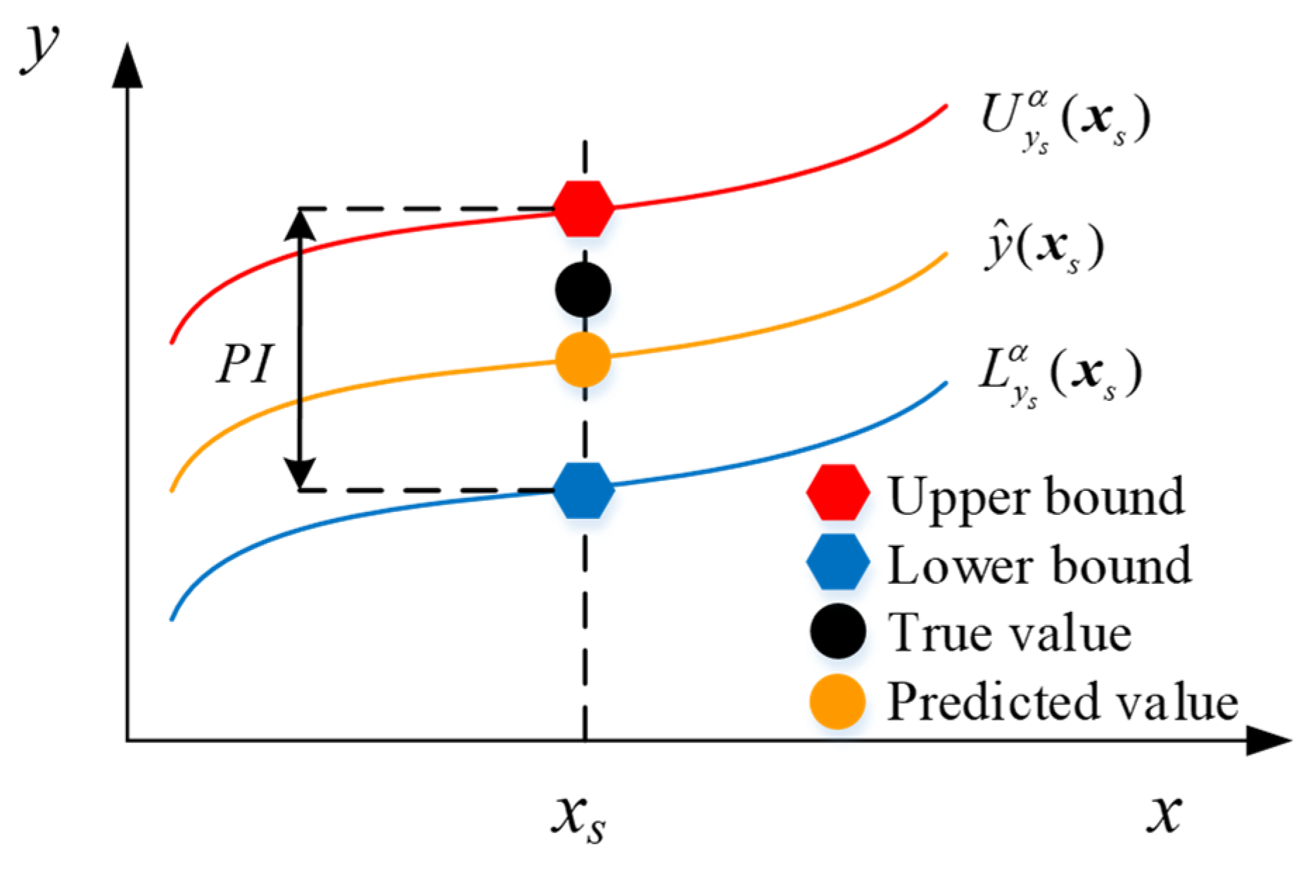
In existing research on arch dam displacement monitoring models, scholars mostly obtain deterministic point estimates of the displacement through mathematical models, with limited consideration for the uncertainty and randomness of displacement changes [11]. Interval prediction contains more informative value compared to point prediction and can reflect the uncertainty based on the prediction interval [26,27]. Therefore, evaluating and quantifying the uncertainty in displacement prediction results is an urgent issue to address.

1.3. Proposed Solution

To address the aforementioned issues, this study integrates mRMR, STL, MF-DFA, and bootstrap methods and, based on CNN-LSTM model, develops a method for predicting displacement intervals for arch dams with cracks. The proposed method is validated using actual displacement data from an arch dam with cracks. The results indicate that the proposed method is reasonable, feasible, and holds significant practical value. The main contributions of this study are as follows:

(1)

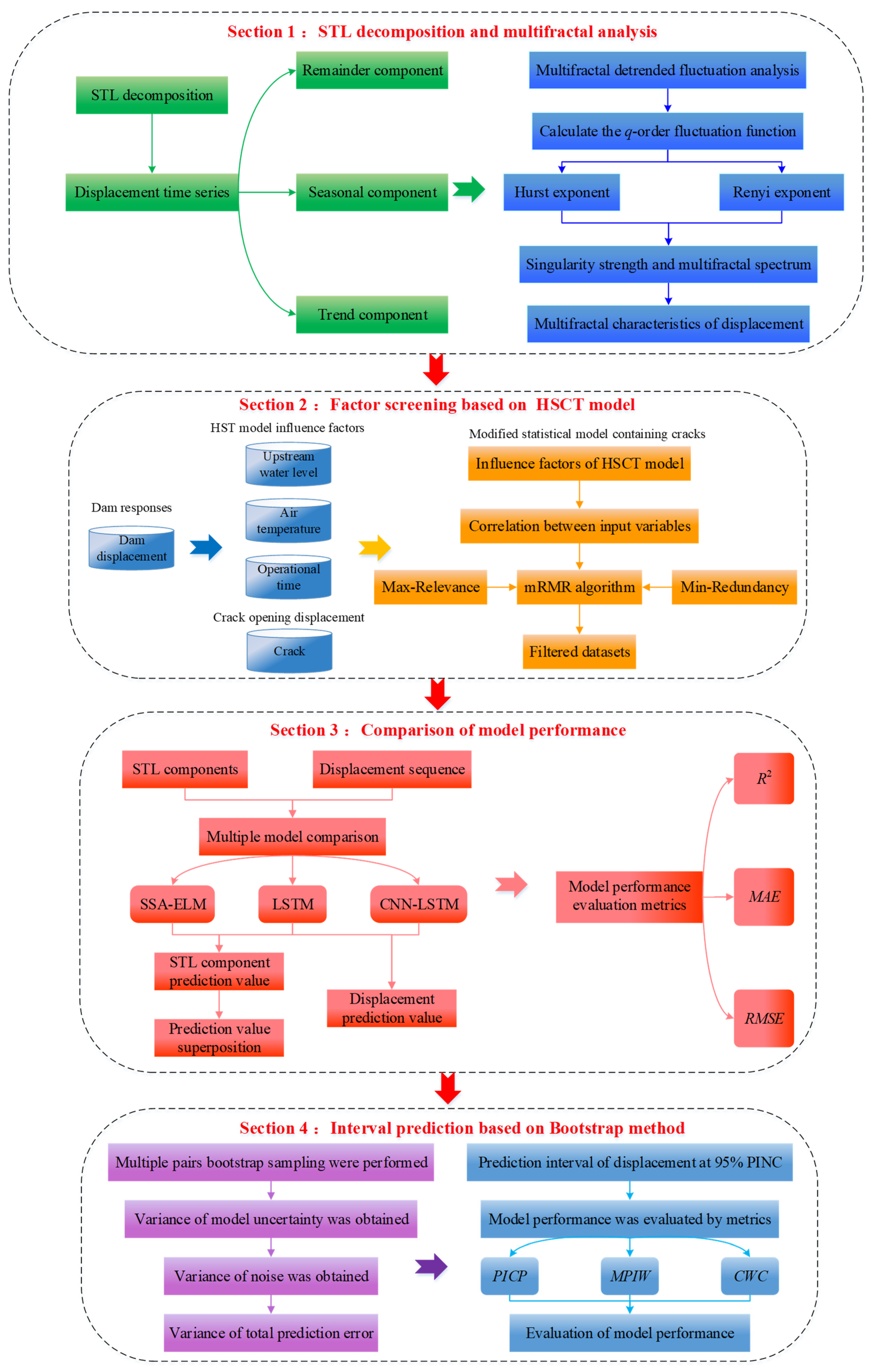
Considering the non-stationarity and time-varying feature of displacement, the STL algorithm is employed to decompose displacement into trend components, seasonal components, and remainder components to implement separate modeling and effectively handle the non-linear characteristics of displacement. Furthermore, the MF-DFA based on multifractal theory is used to analyze the multifractal features of displacement for trend identification.

(2)

Introducing crack opening displacement as a factor that influences the displacement within the HST model, establishing the HSCT model. Utilizing the mRMR method to identify irrelevant variables in the HSCT model, resulting in a screened set.

(3)

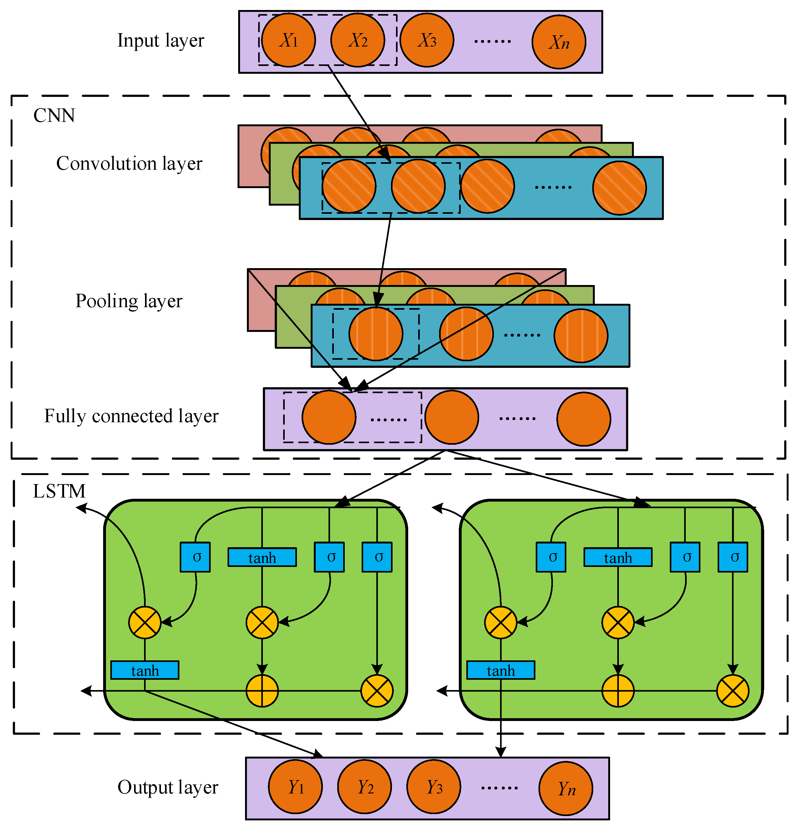
To explore the uncertainty and randomness in displacement changes, and to account for errors in regression models and noise, the study introduces prediction intervals using the bootstrap method and a CNN-LSTM model to quantify the impact of these uncertainty factors and thereby enhance the reliability of displacement predictions.

2. Principles and Methodologies

2.1. Displacement STL Decomposition

Seasonal-trend decomposition using loess (STL) is a time series decomposition algorithm based on Loess smoothing. Due to its simple design and fast computation speed, it is commonly used for handling long time series [14]. The algorithm decomposes the time series into trend components, seasonal components, and remainder components through inner and outer loops:

$$Y_t=T_t+S_t+R_t$$

(1)

where $Y_t$ represents the displacement value at time t, $T_t$ represents the trend component at time t, it represents the long-term direction of change in the time series data and reflects the overall upward or downward trajectory of the data over time. The trend component is typically smooth, removing the effects of short-term fluctuations. $S_t$ represents the seasonal component at time t; it refers to the part of the time series that exhibits periodic variations, usually associated with specific time periods. The seasonal component reflects the repetitive patterns in the data during specific time intervals. $R_t$ represents the remainder component, it refers to what remains in the time series after the trend and seasonal components have been removed. The remainder component includes random fluctuations or noise that cannot be explained by the trend and seasonal elements.

The STL consists of two recursive processes: the inner loop and the outer loop. Let $S_t^k,T_t^k$ denote the seasonal and trend components at the k-th iteration, respectively. The next iteration at k + 1 is carried out as follows:

(1)

Detrend time series by computing the sequence $Y_t-T_t^k$.

(2)

Smooth seasonal subseries by applying Loess smoothing to detrended subseries, resulting in a temporary seasonal series $C_t^{k+1}$.

(3)

Low-pass filter for smoothing a subsequence. Obtained $L_t^{k+1}$ through the use of low-pass filters and the Loess process.

(4)

Compute the seasonal component $S_t^{k+1}$ for k + 1 iteration using the formula $C_t^{k+1}-L_t^{k+1}$.

(5)

Remove the seasonal component pursuant to the expression $Y_t-S_t^{k+1}$.

(6)

Derive the trend component by applying Loess smoothing to the time series obtained in step (5) to obtain the k + 1 iteration’s trend component $T_t^{k+1}$.

In the outer loop, the remainder components are computed using the seasonal and trend components obtained after the inner loop iterations:

$$R_t^{k+1}=Y_t-T_t^{k+1}-S_t^{k+1}$$

(2)

2.2. Multifractal Analysis of Displacement

To analyze the trend changes of displacement sequences, multifractal detrended fluctuation analysis (MF-DFA) is carried out to analyze the three displacement components obtained from STL decomposition and the displacement itself. MF-DFA is an analysis method based on multifractal theory, used to describe the fractal characteristics of time series and analyze their self-similarity and long-memory properties [36,37]. Taking the displacement trend component as an example, the calculation steps of MF-DFA are elaborated as follows.

Given the displacement trend component x(t), with a sequence length of N and a sequence mean of μ_x, then calculate the cumulative deviation sequence y(t) of x(t) relative to μ_x.

$$y(t)={\displaystyle \sum _{i=1}^t(x(i)-{\mu }_x)}$$

(3)

Given a time scale s, divide y(t) into m equally long, non-overlapping subintervals, m = int(N/s). Conduct trend fitting for each subinterval; subtract the trend component from the original data to obtain the residual sequence z_v(t):

$$z_v(t)=y_v(t)-p_v^k(t)$$

(4)

where y_v(t) represent subintervals, $p_v^k(t)$ is a k-th order fitted polynomial for the v-th subinterval.

Calculate F²(s,v) of the residual sequence z_v(t) and the q-th order fluctuation function F_q(s):

$$F^2(s,v)={\displaystyle \frac{1}{s}}{\displaystyle \sum _{t=1}^s{[z_v(t)]}^2}$$

(5)

$$F_q(s)={\left\{{\displaystyle \frac{1}{m}}{\displaystyle \sum }_{v=1}^m{[F^2(s,v)]}^{q/2}\right\}}^{1/q}$$

(6)

By varying the value of s and repeating the above steps, the corresponding F_q(s) can be obtained. If there is long-range correlation in the displacement trend component, the following relationship exists between F_q(s) and s:

$$F_q(s)\propto s^{h(q)}$$

(7)

$$\lg F_q(s)=h(q)\lg s+\lg b$$

(8)

where F_q(s) represents the q order fluctuation function of a sequence, h(q) stands for the Hurst exponent, and b is a constant coefficient. If h(q) is a fixed constant, it indicates that the displacement trend component is monofractal without multifractal features. If h(q) is a non-linear decreasing function of q, then the displacement trend component exhibits multifractal features.

The fractal strength and fractal singularity of the displacement trend component are typically characterized by the multifractal spectrum f(α).

$$\tau (q)=qh(q)-1$$

(9)

$$\alpha =d\tau (q)/dq$$

(10)

$$f(\alpha )=q\alpha -\tau (q)$$

(11)

where τ(q) represents the Renyi exponent, also known as the scaling function. If it is a non-linear, convex function of q, then the displacement trend component exhibits multifractal characteristics. α stands for singularity strength, f(α) for multifractal spectrum. When the α−f(α) relationship is unimodal and convex, resembling a quadratic function, it indicates that the displacement trend component possesses multifractal characteristics.

Moreover, the displacement’s seasonal component, remainder component, and the displacement sequence itself can be analyzed using MF-DFA based on the above steps.

2.3. Establishment of Displacement Factor Set of Arch Dam with Cracks

The commonly used hydrostatic-seasonal-time (HST) model currently attributes displacement changes to the main influences of water pressure, temperature, and time. Additionally, the opening of some horizontal cracks changes with the load, which also significantly affects the dam displacement. Therefore, incorporating crack opening displacements, the hydrostatic-seasonal-crack-time (HSCT) model [10,34,35] can be expressed as:

$$\delta =a_0+{\displaystyle \sum _{i=1}^4{a}_i{H}^i}+{\displaystyle \sum _{j=1}^2\left(b_{1j}\sin \frac{2\pi jt}{365}+b_{2j}\cos \frac{2\pi jt}{365}\right)}+c_1\theta +c_2\ln \theta +{\displaystyle \sum _{k=1}^s{d}_k{J}_k}$$

(12)

where H represents the upstream water depth, $a_0$ is a constant term, $a_i$, $b_{1j}$, $b_{2j}$, $c_1$, $c_2$ and $d_k$ are fitting coefficients, t denotes the cumulative number of days from the displacement observation date to the initial displacement monitoring date, $\theta =t/100$, s is the number of joint meters, and $J_k$ represents the crack opening of each joint meter.

Based on the HSCT regression model, obtain a set of factors that affect displacement, and match these factors with the observed displacement values:

$$(\mathit{X},\mathit{Y})=\left(H,H^2,H^3,H^4,\sin {\displaystyle \frac{2\pi t}{365}},\sin {\displaystyle \frac{4\pi t}{365}},\cos {\displaystyle \frac{2\pi t}{365}},\cos {\displaystyle \frac{4\pi t}{365}},\theta ,\ln \theta ,J_k,y\right)$$

(13)

In the formula, X is the matrix of influencing factors; Y is the target variable, the internal elements are displacement values; and $J_k$ is the crack opening and closing degree measured by the joint meters.

In the HSCT model, multiple collinearity among input variables leads to redundant information among variables, increasing model complexity. Feature selection helps identify a representative subset of variables to replace the original set, aiding in reducing data dimensions and thus lowering model complexity. According to the literature [35], max-relevance and min-redundancy (mRMR) is effective in selecting features for input factors, identifying relatively important variables. For specific details of this method, refer to literature [38].

2.4. Displacement Prediction Based on CNN-LSTM

CNN extracts features from input data through convolutional kernels and obtains output through non-linear activation functions. The pooling layer follows the convolutional layer to reduce feature dimensionality, thereby reducing redundant information and computational complexity [39]. LSTM introduces storage units in recurrent neural networks (RNNs) to ensure that data passing through does not ignore dependencies between data. LSTM has three types of gate structures: forget gate, input gate, and output gate. For specific details of LSTM, refer to reference [21].

In the CNN-LSTM model, CNN is used to extract local features: (1) Short-term trends: identifying the upward or downward trends in data values within a short time window. (2) Local periodicity: detecting local periodic changes within smaller time frames. These features can provide rich information for the subsequent LSTM layers, helping to capture the long-term dependencies and evolving trends in time series data. While LSTM is utilized for modeling long-term dependencies. The model includes an input layer, convolutional layer, LSTM layer, and output layer, as shown in Figure 1: (1) Input layer: receives displacement data and its influencing factors. (2) Convolution layer: comprises 1D convolution layers, batch normalization, ReLU activation, pooling, and fully connected layers to extract features from displacement data. It enhances performance, addresses the vanishing gradient problem, and reduces computational complexity. (3) LSTM layer: processes output displacements from the convolution layer to learn feature vectors, exploring latent information and improving training efficiency through non-linear activation. (4) Output layer: flattens and processes LSTM output through fully connected layers for final output.

This article uses the Adam optimizer instead of the traditional gradient descent strategy for hyperparameter updating. The Adam optimizer efficiently handles sparse gradient problems and prevents excessive parameter updates [40]. During model training, the loss function is mean squared error (MSE), and performance of the predictive model is evaluated using root mean square error (RMSE), mean absolute error (MAE), and coefficient of determination (R²).

$$RMSE=\sqrt{{\displaystyle \frac{1}{n}}{\displaystyle \sum _{i=1}^n{(y_m^i-y_p^i)}^2}}$$

(14)

$$MAE={\displaystyle \frac{1}{n}}{\displaystyle \sum _{i=1}^n\left|y_m^i-y_p^i\right|}$$

(15)

$$R^2={\displaystyle \frac{{({\displaystyle \sum _{i=1}^n(y_m^i-{\overline{y}}_m)}(y_p^i-{\overline{y}}_p))}^2}{{\displaystyle \sum _{i=1}^n{(y_m^i-{\overline{y}}_m)}^2}{\displaystyle \sum _{i=1}^n{(y_p^i-{\overline{y}}_p)}^2}}}$$

(16)

where n represents the number of predicted data, $y_m^i$ and $y_p^i$ denote the i-th monitoring data and predicted data, and ${\overline{y}}_m$ and ${\overline{y}}_p$ denote the mean values of both the observed and the predicted data.

2.5. Displacement Interval Prediction Based on Bootstrap

The displacement of a dam is influenced by various factors, and the measured displacement exhibits a certain degree of randomness. The diagram in Figure 2 illustrates the prediction interval, which provides more information for the operation and management of the dam, thereby improving the reliability of predictions. Predicting dam displacements is a regression problem, where input factor vectors x_s and output targets y_s always appear in pairs. To account for the uncertainty of displacement evolution, the pairs bootstrap method is applied to predict intervals for the superposition displacements in Section 2.4, as detailed in reference [41].

Assuming that the estimation error and data noise are statistically independent, the variance of the total prediction error can be calculated as follows:

$${\sigma }_y^2({\mathit{x}}_s)={\sigma }_{\widehat{F}}^2({\mathit{x}}_s)+{\sigma }_{\xi }^2({\mathit{x}}_s)$$

(17)

where ${\sigma }_{\widehat{F}}^2({\mathit{x}}_s)$ and ${\sigma }_{\xi }^2({\mathit{x}}_s)$ represent the variance of model uncertainty and data noise, respectively.

When the significance level is set to α, $(1-\alpha )\times 100\%$ is known as the prediction interval nominal confidence level (PINC). The displacement y_s at the s-th time step can be represented:

$$I_{y_s}^{\alpha }({\mathit{x}}_s)=\left[L_{y_s}^{\alpha }({\mathit{x}}_s),U_{y_s}^{\alpha }({\mathit{x}}_s)\right]$$

(18)

$$L_{y_s}^{\alpha }({\mathit{x}}_s)=\widehat{F}({\mathit{x}}_s)-z_{1-\alpha /2}\sqrt{{\sigma }_{y_s}^2({\mathit{x}}_s)}$$

(19)

$$U_{y_s}^{\alpha }({\mathit{x}}_s)=\widehat{F}({\mathit{x}}_s)+z_{1-\alpha /2}\sqrt{{\sigma }_{y_s}^2({\mathit{x}}_s)}$$

(20)

where $L_{y_s}^{\alpha }({\mathit{x}}_s)$ and $U_{y_s}^{\alpha }({\mathit{x}}_s)$ are respectively the lower and upper bounds of the displacement prediction interval, $\widehat{F}({\mathit{x}}_s)$ denotes the output of the prediction model, ${\sigma }_{y_s}^2({\mathit{x}}_s)$ denotes the variance of the total prediction error, $z_{1-\alpha /2}$ denotes the percentile of the standard normal distribution, depending on the specified significance level (usually 0.05).

To assess the overall quality of the constructed interval, the prediction interval coverage probability (PICP), the mean prediction interval width (MPIW), and the coverage width-based criterion (CWC) are introduced to measure [42]. Its definitions are as follows:

$$PICP={\displaystyle \frac{1}{N_t}}{\displaystyle \sum _{s=1}^{N_t}{c}_s},c_s=\left\{\begin{array}{l}1,y_s\in \left[L_{y_s}^{\alpha }({\mathit{x}}_s),U_{y_s}^{\alpha }({\mathit{x}}_s)\right]\hfill \\ 0,y_s\notin \left[L_{y_s}^{\alpha }({\mathit{x}}_s),U_{y_s}^{\alpha }({\mathit{x}}_s)\right]\hfill \end{array}\right.$$

(21)

$$MPIW={\displaystyle \frac{1}{N_t}}{\displaystyle \sum _{s=1}^{N_t}\left[U_{y_s}^{\alpha }({\mathit{x}}_s)-L_{y_s}^{\alpha }({\mathit{x}}_s)\right]}$$

(22)

$$CWC=MPIW[1+\gamma (PICP)e^{-\eta (PICP-PINC)}]$$

(23)

$$\gamma (PICP)=\left\{\begin{array}{l}0,PICP\ge PINC\\ 1,PICP\le PINC\end{array}\right.$$

(24)

where N_t represents the number of samples. The value of c_s is 1 if the displacement lies within the interval, and 0 otherwise; $\gamma (PICP)$ serves as a control factor and $\eta$ is a penalization parameter. When PICP is greater than or equal to the PINC, the exponential term is eliminated, thus the quality of the interval is solely gauged by the MPIW. Conversely, if the PICP is less than the PINC, a penalty is imposed, and in this paper, the parameter is set to 50 [26].

2.6. Displacement Interval Prediction Method

Drawing on the aforementioned principles, this section delineates the detailed execution of the proposed approach. The workflow is depicted in Figure 3. The methodology primarily encompasses the subsequent steps:

Step 1: The displacement sequence is decomposed into trend components, seasonal components, and remainder components using STL decomposition. Based on fractal theory, the MF-DFA method is utilized to calculate the Hurst exponent, Renyi exponent, and multifractal spectrum of displacement components and displacement sequence itself, enabling a multifractal analysis of displacement and its components to achieve qualitative analysis of displacement trends.

Step 2: Based on the HST model, crack is considered as a factor affecting displacement, thus establishing the HSCT model. Due to information redundancy in the HSCT model, the variable selection method mRMR is used to select the factors affecting displacement, resulting in a set of selected displacement factors.

Step 3: Based on the selected set of displacement factors obtained in Step 2, matched with displacement components in Step 1 to form a dataset. A deep learning model (CNN-LSTM) is established to predict displacement trend components, seasonal components, and remainder components; then the predictions are combined to obtain the final displacement prediction, achieving quantitative displacement prediction. Additionally, predictions are made for the displacement sequence itself, and model performance is evaluated based on evaluation metrics. For comparative purposes, SSA-ELM and LSTM predictions are also performed.

Step 4: To quantify the impact of uncertainty factors on displacement, the three models mentioned above are used to implement interval predictions based on the bootstrap method. This involves estimating the variance of uncertainty in the combined displacement, noise variance, and uncertainty variance in the noise regression model, ultimately obtaining the prediction interval at a 95% confidence level and calculating evaluation metrics to compare the performance of prediction intervals for each model.

3. Engineering Instance

Taking a certain gravity arch dam on the upstream of the Qingyi River, a tributary of the Yangtze River in China, as the research subject, Figure 4 shows the spatial distribution of the vertical line measuring points of the arch dam [11]. According to references [6,7], the horizontal cracks at an elevation of 105 m downstream of the dam, with a depth of about 6 m, which is relatively deep and has a significant impact on the displacement of the dam body above an elevation of 105 m, as illustrated in Figure 5. Therefore, this study focuses on the impact of horizontal cracks at an elevation of 105 m downstream of the dam on the displacement. The evolution of the crack is primarily reflected through its length, depth, and opening displacement. In practical engineering, the opening displacement is the main parameter monitored. This study selected measuring points PL8−U and PL18−U near the elevation of 105 m to analyze the horizontal displacements from 1 January 2006 to 31 December 2015.

The water level and temperature data are obtained through sensors installed on the arch dam, while the displacements are obtained based on sensors installed on the vertical observation system. Figure 6 illustrates the variations in water level, temperature, and displacement near the 105 m elevation PL8−U and PL18−U throughout the entire time period. The crack opening displacement process lines of the selected 19 joint meters are shown in Figure 7. Both displacement and temperature display evident periodic patterns, with displacement demonstrating an inverse relationship with temperature. A decrease in temperature leads to downstream displacement of the arch dam, while an increase in temperature results in upstream displacement, aligning with the deformation behavior of the arch dam.

4. Multifractal Characteristics Analysis

Addressing the non-linearity and non-stationary characteristics of data disturbed by noise, the use of the STL algorithm decomposes the displacement of measuring points into trend components, seasonal components, and remainder components. Figure 8 displays the STL decomposition results for PL8−U and PL18−U. As depicted in Figure 8, both measuring points exhibit a growing trend in their trend components, while the seasonal components of both points demonstrate strong periodicity. Furthermore, the remainder components of the two measuring points lack a clear pattern [43].

To further analyze the trend of displacement, MF-DFA is applied to analyze the three displacement components obtained from STL decomposition and the displacement itself, with the fluctuation order q ranging from [−10, 10]. The analysis results are shown in Figure 9, Figure 10 and Figure 11.

Figure 9 illustrates the variation of the Hurst exponent for displacement and its components. It can be observed from Figure 9 that as q fluctuates within the range of [−10, 10], the Hurst exponent of the displacement and its components is not a constant but exhibits a non-linearly decreasing trend with the variation of q. This indicates that the displacement and its components possess distinct multifractal characteristics. Under different orders of fluctuation q, the Hurst exponent curves are concentrated in the lower part, showing weaker multifractality, yet the h(q) values are significantly greater than 0.5, suggesting that the displacement and its components have good memory and long-range correlation, embodying both non-stationarity and randomness. From Figure 9, it is evident that when q < 0, the distribution of h(q) values for displacement and its components is more dispersed, with a noticeable difference in the strength of positive persistence. Conversely, when q > 0, the h(q) values show better consistency, with similar positive persistence. Moreover, the difference in h(q) values when q > 0 is smaller than when q < 0, indicating that the decreasing trend of displacement and its components is essentially the same, with a consistent overall trend and stable long-range correlation. Based on h(q), the Renyi exponent, that is, the scaling function τ(q), is calculated, as shown in Figure 10. The scaling functions of the displacement and its components exhibit good consistency, with a convex shape in the middle, satisfying τ(0) = −1, and are overall non-linear, further confirming the multifractal characteristics of the displacement. Figure 11 presents the multifractal spectrum, where each multifractal spectrum image shows a single-peak convex distribution, resembling a quadratic function curve, depicting the diversity of local changes at different moments. The singularity strength α is mainly concentrated on both sides of the image, reflecting the uneven distribution of the fractal structure of the displacement sequence, and the uneven distribution of α also corroborates the multifractal characteristics of the measurement sequence. Regardless of whether it is displacement or its components, the multifractal spectrum is essentially symmetric, with good overall coordination and stable development, and reflects the multifractal characteristics of the displacement sequence. The aforementioned analysis indicates that the variation of the displacement and its components shows a consistent and gradually ascending trend, with self-similarity and regularity [44]. Furthermore, compared to direct multifractal analysis of displacement, multifractal analysis of the trend and seasonal components after STL decomposition also yields the same conclusion.

5. Results and Analysis

5.1. Construction of Influencing Factor Set

This study introduces the crack opening displacement as a factor in HST model, resulting in the HSCT model. The set of displacement influence factors can be denoted as $\{H,H^2,H^3,H^4,\sin {\displaystyle \frac{2\pi t}{365}},\sin {\displaystyle \frac{4\pi t}{365}},\cos {\displaystyle \frac{2\pi t}{365}},\cos {\displaystyle \frac{4\pi t}{365}},\theta ,\ln \theta ,J\}$, where $J=\{J_1,J_2,\dots ,J_{19}\}$ represents all crack factors. To further verify the necessity of considering cracks, this paper implemented multi model prediction analysis of displacement of two measuring points under the HST model and HSCT model.

Table 1. Improvement rates of two measuring points under HSCT model.

Monitoring Points	Models	RMSE	MAE	R2
PL8−U	SSA-ELM	0.264 (10.5%)	0.188 (12.2%)	0.912 (2.4%)
	LSTM	0.238 (15.3%)	0.168 (18.1%)	0.929 (3.1%)
	CNN-LSTM	0.236 (11.6%)	0.165 (15.8%)	0.931 (2.2%)
PL18−U	SSA-ELM	0.267 (12.7%)	0.214 (8.5%)	0.912 (3.1%)
	LSTM	0.262 (6.1%)	0.213 (5.3%)	0.914 (1.3%)
	CNN-LSTM	0.258 (5.5%)	0.212 (4.5%)	0.917 (1.1%)

shows the improvement rate of the HSCT model compared to HST model prediction.

According to Table 1, compared to the HST model, the HSCT model considering the influence of cracks has higher prediction accuracy, with an average RMSE reduction of 11.6% and an average MAE reduction of 10.4% for the SSA-ELM model; the RMSE of the LSTM model decreased by an average of 10.7%, and the MAE decreased by an average of 11.7%; the RMSE of the CNN-LSTM model decreased by an average of 8.6%, and the MAE decreased by an average of 8.7%. The validation of various models mentioned above shows that using the factor set under the HSCT model for prediction has improved accuracy and further enhanced model performance, which confirms the necessity of considering the influence of cracks. Based on the conclusion in reference [37], the mRMR method was used for feature selection. Factors corresponding to a mutual information quotient less than 1 were eliminated to obtain the filtered factor set.

Table 2. HSCT model factors of PL8−U and PL18−U calculated by mRMR.

Factor	PL8−U	PL18−U	Factor	PL8−U	PL18−U
x1	3.947	1.266	J6	1.527	1.390
x2	1.108	2.885	J7	0.864	0.531
x3	1.528	0.838	J8	1.527	1.390
x4	0.875	0.662	J9	1.584	1.442
x5	19.641	17.617	J10	3.042	5.740
x6	1.701	1.002	J11	0.583	0.772
x7	4.540	10.262	J12	5.069	1.389
x8	34.841	1.329	J13	0.625	0.569
x9	1.528	1.389	J14	5.456	10.563
x10	0.735	0.669	J15	1.527	1.388
J1	7.400	6.787	J16	18.267	4.252
J2	5.074	1.390	J17	0.639	0.581
J3	1.528	1.389	J18	0.862	1.402
J4	3.044	2.764	J19	5.078	1.390
J5	1.005	12.943	-	-	-

shows the results of PL8−U and PL18−U calculated using mRMR under the HSCT model.

For measuring point PL8−U, after mRMR calculation, the water pressure factor H⁴ and the aging factor lnθ were removed, and the crack factors J₁–J₆, J₈–J₁₀, J₁₂, J₁₄–J₁₆, and J₁₉ were selected. For measuring point PL18−U, after mRMR calculation, the water pressure factors H³ and H⁴, the aging factor lnθ were removed, and the crack factors J₁–J₆, J₈–J₁₀, J₁₂, J₁₄–J₁₆, J₁₈, and J₁₉ were selected.

Table 3. Subsets of factors through mRMR method.

Monitoring Points	Filtered Data Sets
PL8−U	{x1–x3, x5–x9, J1–J6, J8–J10, J12, J14–J16, J19}
PL18−U	{x1, x2, x5–x9, J1–J6, J8–J10, J12, J14–J16, J18, J19}

shows the final factor sets for different measuring points after variable selection.

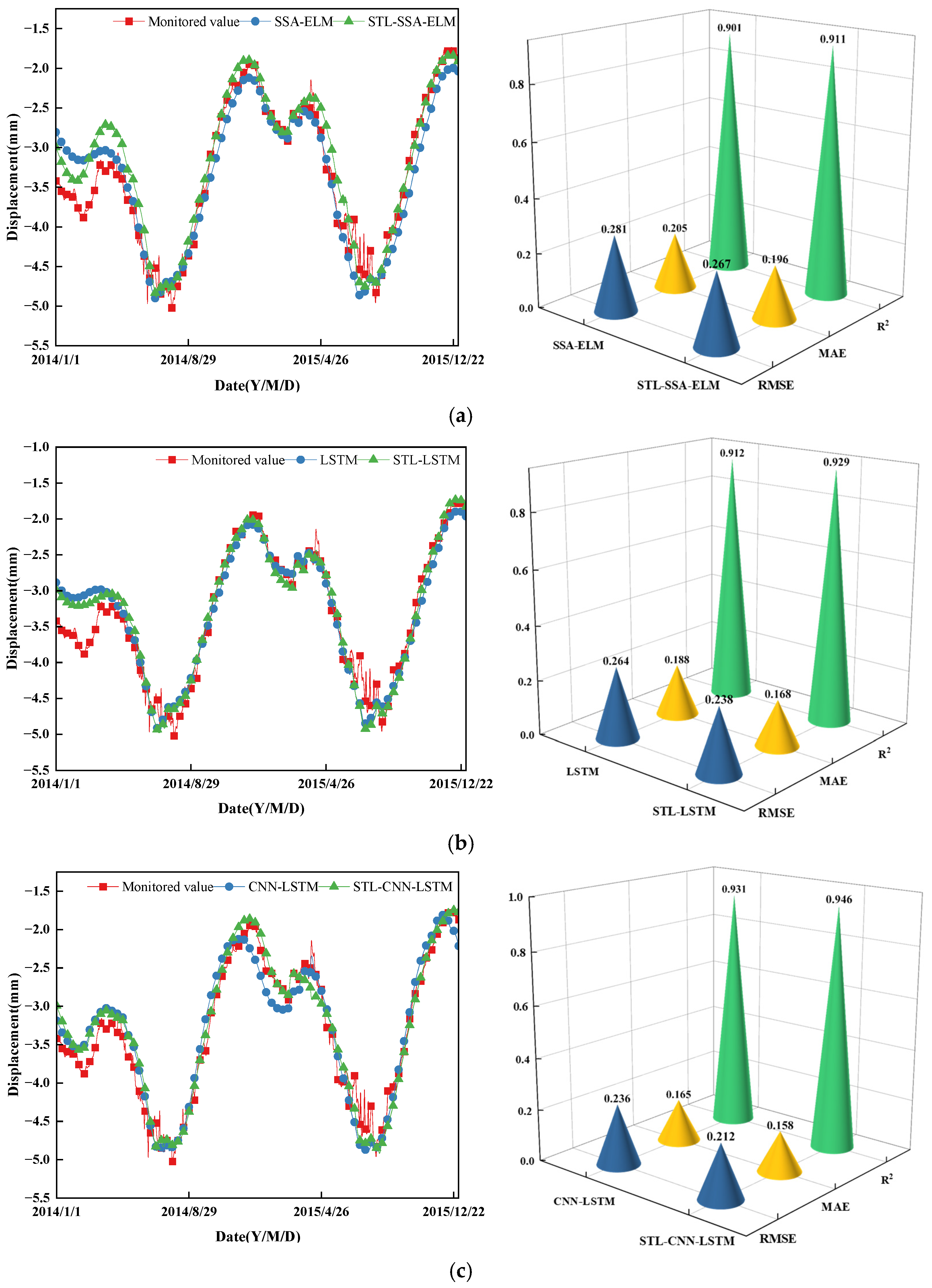
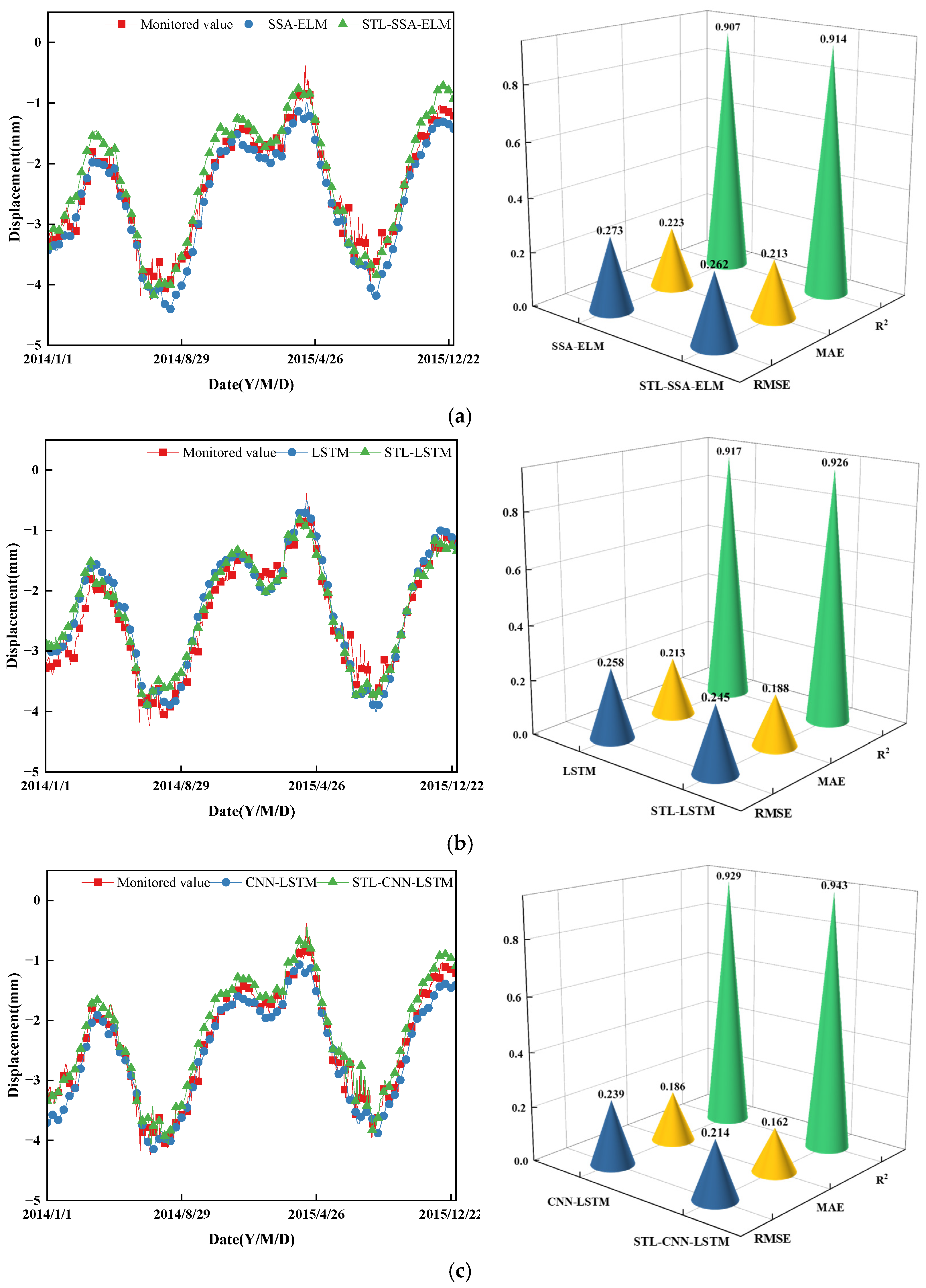
5.2. Comparison of Prediction Model Performance

To affirm the efficacy of STL decomposition in enhancing the separative modeling process, models such as SSA-ELM, LSTM, and CNN-LSTM were constructed to predict the individual components derived from STL decomposition. The subsequent aggregation of these predictions yields the superposition displacement. For comparison purposes, the point value prediction of the displacement without undergoing STL decomposition was also performed using the three models mentioned above. The first 80% of the dataset was used as the training set for the models, while the remaining 20% was used as the testing set to evaluate model accuracy. Figure 12 and Figure 13 display the multi-model fitting curves and their statistical indicators for the test sets of two measuring points.

Analyzing the fitting curves and statistical metrics presented in Figure 12 and Figure 13, it is evident that the CNN-LSTM model achieves a notable decrease in error measures compared to the SSA-ELM, with an average reduction of 16.9% in the RMSE and 19.8% in the MAE. Furthermore, when compared with the LSTM model, the CNN-LSTM demonstrates an average decrease of 10.4% in RMSE and 11.1% in MAE. The CNN-LSTM emerges as the superior model, underscoring its proficiency in managing complex, high-dimensional, non-linear dynamics. The analysis above indicates that decomposing displacement through STL, modeling the components separately, and combining them yields improved predictive accuracy compared to directly predicting displacement, thus validating the necessity of STL decomposition.

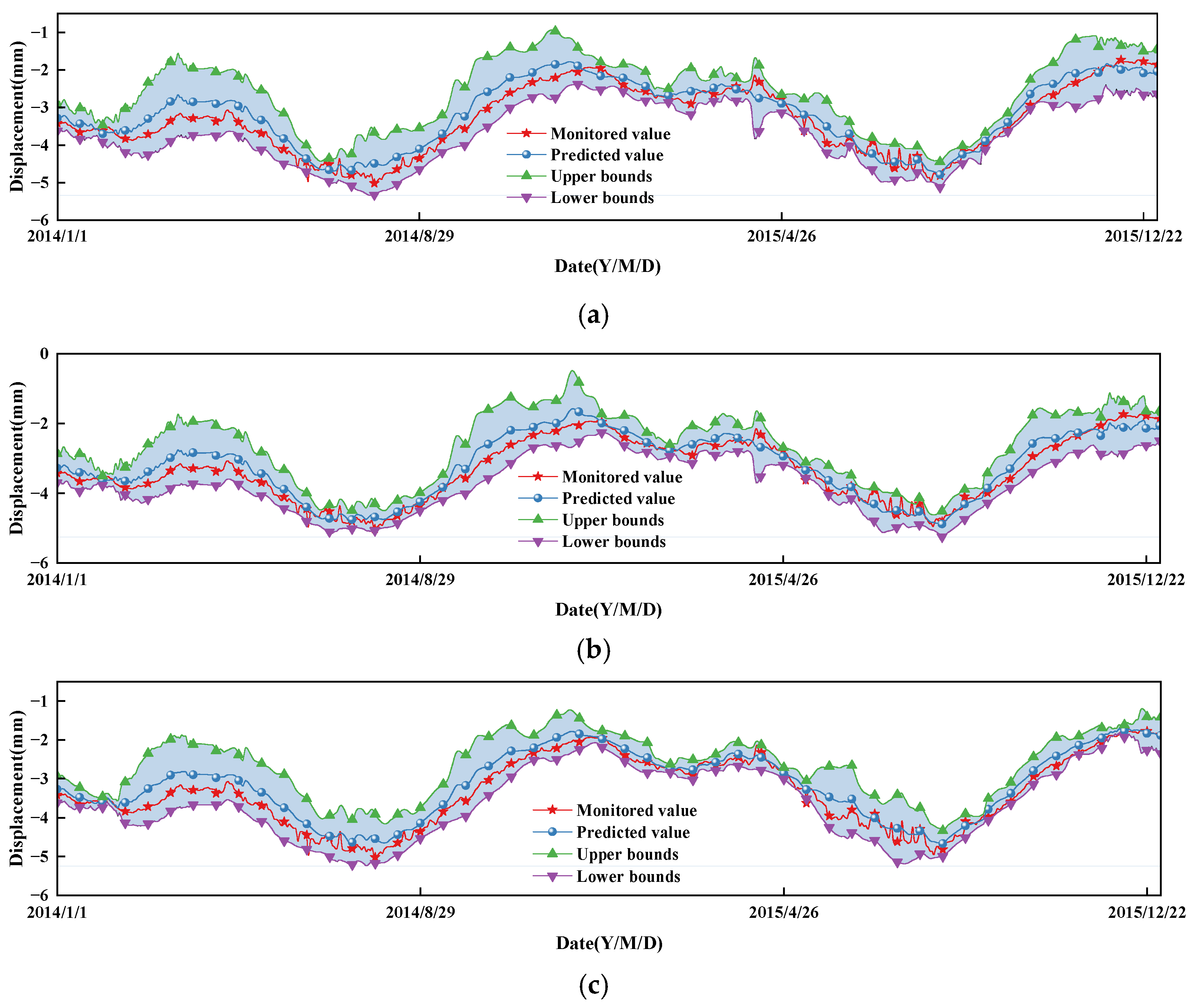
5.3. Displacement Interval Prediction Analysis

Traditional point value prediction methods only output deterministic values as the final prediction outcome, but interval prediction can construct high-confidence intervals to represent the uncertainty of displacement. The goal of interval prediction is to construct a dam displacement prediction interval with a certain level of confidence to ensure an accurate understanding of the dam’s operational state. To study the performance of different prediction algorithms in quantifying the impact of uncertainty, this study implemented SSA-ELM, LSTM, and CNN-LSTM models based on the bootstrap method for interval prediction at a 95% confidence level. Figure 14 and Figure 15 provide the prediction intervals for two measuring points.

Table 4. Performance metrics for interval prediction of two measuring points.

Measuring Points	Prediction Models	PINC 95%
		PICP (%)	MPIW (mm)	CWC (mm)
PL8−U	STL-SSA-ELM	98.22	1.10	1.10
	STL-LSTM	98.89	0.98	0.98
	STL-CNN-LSTM	98.77	0.95	0.95
PL18−U	STL-SSA-ELM	95.79	1.07	1.07
	STL-LSTM	98.49	1.21	1.21
	STL-CNN-LSTM	98.90	1.11	1.11

shows the quantitative evaluation metrics for interval prediction of the displacements at two measuring points across multiple models.

Table 4 further demonstrates that the constructed prediction intervals can cover the vast majority of samples. At a 95% confidence level, the PICP values of the three models are all greater than the specified PINC (95%), indicating that CWC will not be affected by penalty terms as PICP exceeds PINC, resulting in relatively small values equal to MPIW. This implies that the obtained prediction intervals are all effective. For the monitoring point PL8−U, the coverage rates of the three models are as high as 98%. The MPIW of SSA-ELM is greater than the other two models, while CNN-LSTM has the smallest MPIW among the three models. For monitoring point PL18−U, the MPIW of SSA-ELM is smaller than the other two models, and the coverage rate is slightly higher than PINC. Although the coverage of LSTM exceeds that of SSA-ELM, its MPIW will inevitably increase. In contrast, CNN-LSTM has the highest coverage and relatively small MPIW. The prediction results of CNN-LSTM are relatively consistent with the true values, allowing for narrower prediction intervals. These results indicate that different prediction algorithms exhibit variations in uncertainty quantification. However, interval prediction based on the bootstrap method and CNN-LSTM model presents satisfactory performance by accurately quantifying the uncertainty of displacement changes.

The complexity of dam systems and limitations in people’s understanding create uncertainties in predicting the displacement of arch dams. In comparison to point value predictions, interval predictions contain more information and can reflect the uncertainties based on the prediction intervals. The proposed method for interval prediction of displacement in arch dams with cracks not only qualitatively analyzes the trend of displacement changes but also quantitatively assesses the accuracy of displacement prediction. This method can effectively replace traditional point-value prediction methods, providing management personnel with more valuable insights to enhance the effectiveness and reliability of dam risk management.

6. Conclusions

There is limited consideration of the impact of cracks on arch dam displacement in existing models and the failure to simultaneously analyze the non-stationarity and uncertainty of displacement. To solve this problem, firstly, crack opening displacement is added to the factors affecting displacement, and a displacement monitoring model HSCT considering the influence of cracks is constructed. The mRMR algorithm is then utilized for feature selection. Subsequently, the displacement is decomposed using the STL method to extract trend components, seasonal components, and remainder components. The multifractal features of displacement are analyzed using MF-DFA. Finally, to account for the uncertainty of displacements, a displacement interval prediction method for arch dams with cracks is developed based on the bootstrap method and the CNN-LSTM model. The superiority of this method is validated using actual displacement data from a specific arch dam with cracks. The main conclusions are as follows:

(1)

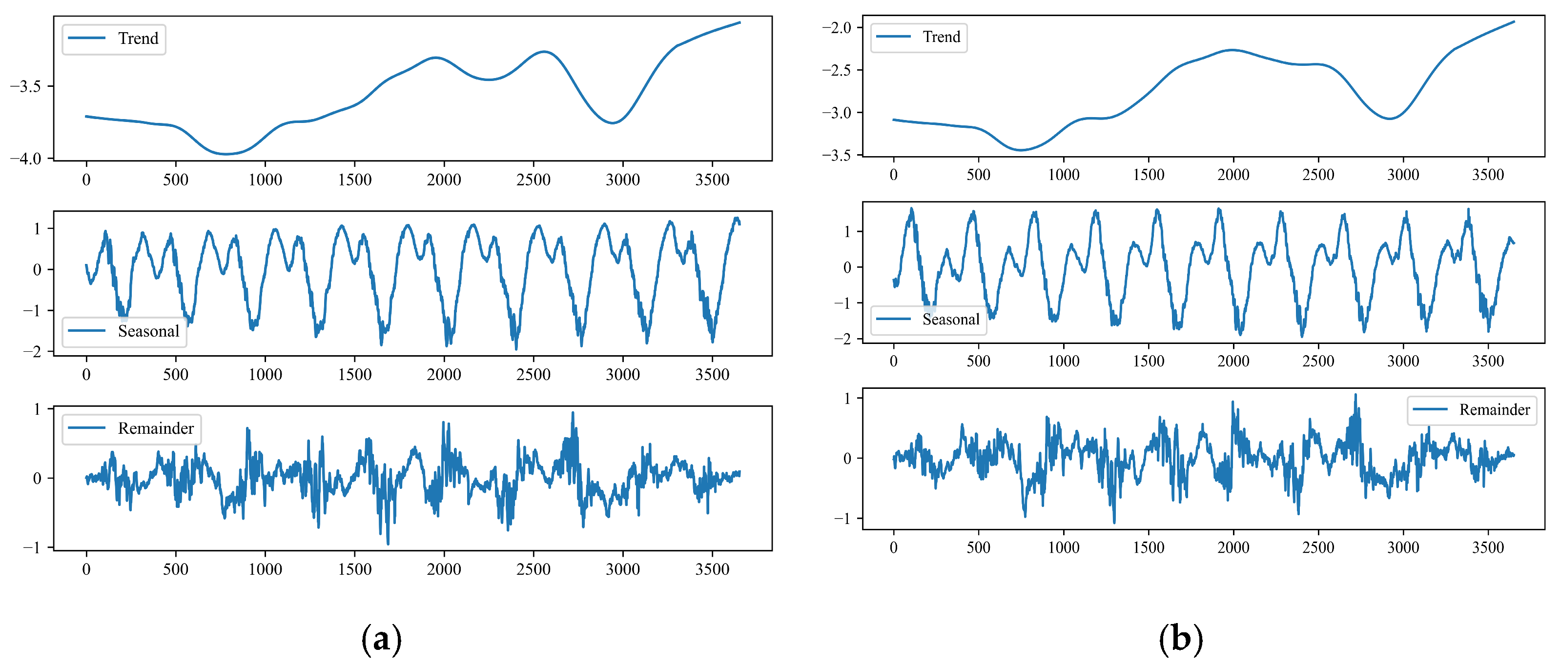
Noise in data often degrades the quality of displacement monitoring sequences and masks actual patterns in displacement sequences. By decomposing displacement sequences into trend components, seasonal components, and remainder components using the STL algorithm, growth trends in trend components, strong periodicity in seasonal components, and irregularity in remainder components are identified. By separating modeling, enabling better handling of the non-linear features of displacement in subsequent prediction and improving prediction accuracy.

(2)

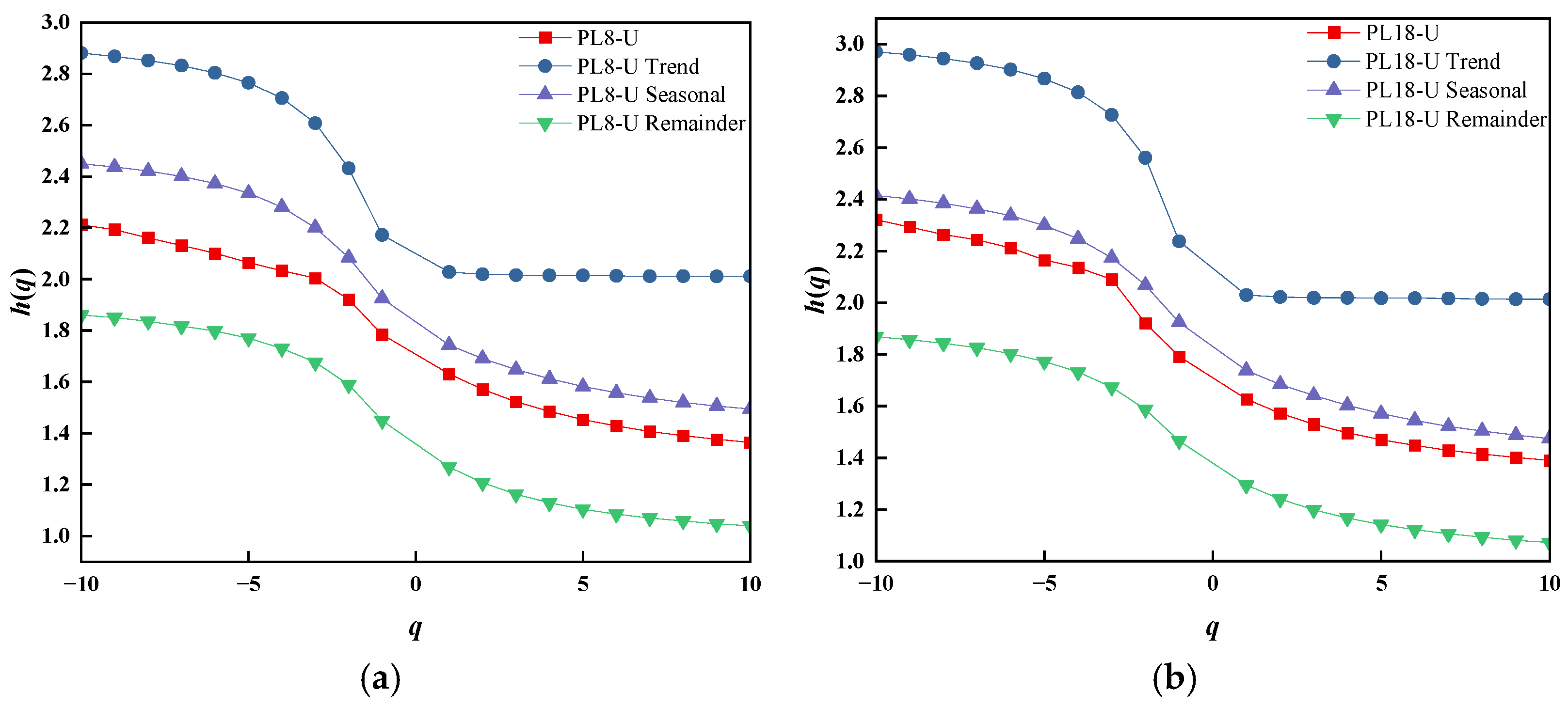
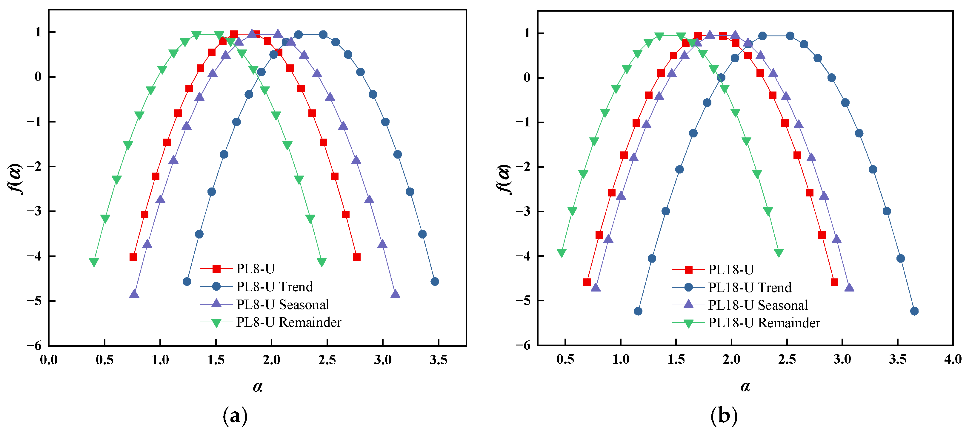
To identify the non-linear dynamic evolution patterns of displacement, the Hurst exponent, Renyi exponent, and multifractal spectrum of displacement and its components are computed using MF-DFA based on multifractal theory. These calculations verify the distinct multifractal features and long-range correlations of displacement and its components, with components exhibiting fractal features consistent with those of displacement. The evolution of displacement is highly complex, and MF-DFA can characterize fractal features at different time scales to effectively identify changing trends in displacement and its components.

(3)

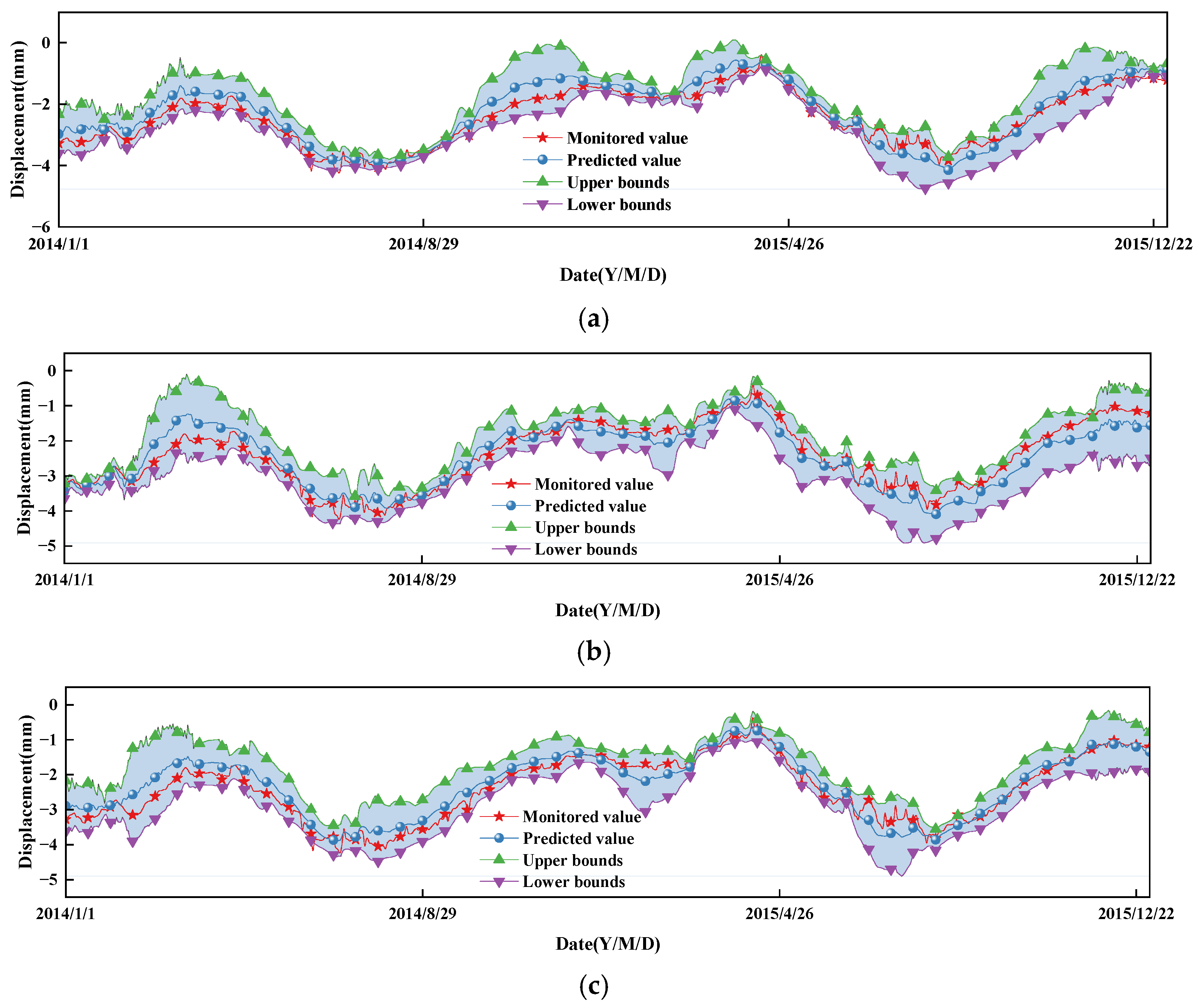
In comparison to deterministic point value predictions, interval predictions contain more information and reflect uncertainty based on the predicted interval. To study the performance of different prediction algorithms in quantifying uncertainty, SSA-ELM, LSTM, and CNN-LSTM models are implemented for interval prediction based on STL decomposition, separate modeling, and superposition. The prediction intervals constructed by these models at a 95% confidence level are effective (PICP ≥ PINC), with CNN-LSTM showcasing the highest performance, achieving a PICP of 98% and the smallest MPIW. This precise quantification of displacement uncertainty through interval prediction enhances the understanding of displacement variations.

(4)

The proposed displacement interval prediction method for arch dams with cracks presents an effective and feasible approach for concrete dam displacement monitoring and health diagnosis. It facilitates both qualitative analysis of displacement trends and quantitative assessment of displacement prediction accuracy, offering a novel perspective for displacement analysis and prediction in hydraulic structures. This method provides valuable insights for operational management personnel, thereby enhancing the reliability of dam risk management.

Although the proposed method and model provide higher accuracy for predicting displacement intervals of arch dams with cracks, there is still room for further improvement. Due to the lack of transparency in the training process of deep learning models, it is necessary to incorporate some interpretation methods in the future, such as the attention mechanism or SHapley Additive exPlanation in references [15,20], to quantitatively analyze the importance of water pressure, temperature, aging, and cracks on displacement and further improve the interpretability of the model.

References

1. Ren, Q.; Li, M.; Kong, T.; Ma, J. Multi-sensor real-time monitoring of dam behavior using self-adaptive online sequential learning. Autom. Constr. 2022, 140, 104365. [Google Scholar] [CrossRef]
2. Lin, C.; Chen, S.; Hariri-Ardebili, M.A.; Li, T. An explainable probabilistic model for health monitoring of concrete dam via optimized sparse bayesian learning and sensitivity analysis. Struct. Control Health Monit. 2023, 2023, 2979822. [Google Scholar] [CrossRef]
3. Huang, B.; Kang, F.; Li, J.; Wang, F. Displacement prediction model for high arch dams using long short-term memory based encoder-decoder with dual-stage attention considering measured dam temperature. Eng. Struct. 2023, 280, 115686. [Google Scholar] [CrossRef]
4. Qin, X.; Guo, J.; Gu, C.; Chen, X.; Xu, B. A discrete-continuum coupled numerical method for fracturing behavior in concrete dams considering material heterogeneity. Constr. Build. Mater. 2021, 305, 124741. [Google Scholar] [CrossRef]
5. Zhao, E.; Li, B. Evaluation method for cohesive crack propagation in fragile locations of RCC dam using XFEM. Water 2020, 13, 58. [Google Scholar] [CrossRef]
6. Zheng, C. Numerical Simulation of Interfaces in Concrete Dams and Its Application; China Institute of Water Resources and Hydropower Research: Beijing, China, 2006. (In Chinese) [Google Scholar]
7. Zhang, G.; Liu, Y.; Zheng, C.; Feng, F. Simulation of influence of multi-defects on long-term working performance of high arch dam. Sci. China Technol. Sci. 2011, 54 (Suppl. S1), 1–8. [Google Scholar] [CrossRef]
8. Chen, S.; Gu, C.; Lin, C.; Hariri-Ardebili, M.A. Prediction of arch dam deformation via correlated multi-target stacking. Appl. Math. Model. 2021, 91, 1175–1193. [Google Scholar] [CrossRef]
9. Wang, S.; Xu, Y.; Gu, C.; Xia, Q.; Hu, K. Two spatial association-considered mathematical models for diagnosing the long-term balanced relationship and short-term fluctuation of the deformation behaviour of high concrete arch dams. Struct. Health Monit. 2020, 19, 1421–1439. [Google Scholar] [CrossRef]
10. Wu, Z. Safety Monitoring Theory and Its Application of Hydraulic Structures; Higher Education Press: Beijing, China, 2003. (In Chinese) [Google Scholar]
11. Chen, H.; Chen, X.; Guan, J.; Zhang, X.; Guo, J.; Yang, G.; Xu, B. A combination model for evaluating deformation regional characteristics of arch dams using time series clustering and residual correction. Mech. Syst. Signal Process. 2022, 179, 109397. [Google Scholar] [CrossRef]
12. Zhou, Y.; Bao, T.; Li, G.; Shu, X.; Li, Y. Multi-expert attention network for long-term dam displacement prediction. Adv. Eng. Inform. 2023, 57, 102060. [Google Scholar] [CrossRef]
13. Hu, J.; Li, X. A novel prediction model construction and result interpretation method for slope deformation of deep excavated expansive soil canals. Expert Syst. Appl. 2024, 236, 121326. [Google Scholar] [CrossRef]
14. Li, M.; Shen, Y.; Ren, Q.; Li, H. A new distributed time series evolution prediction model for dam deformation based on constituent elements. Adv. Eng. Inform. 2019, 39, 41–52. [Google Scholar] [CrossRef]
15. Lei, W.; Wang, J. Dynamic Stacking ensemble monitoring model of dam displacement based on the feature selection with PCA-RF. J. Civ. Struct. Health Monit. 2022, 12, 557–578. [Google Scholar] [CrossRef]
16. Ren, Q.; Li, H.; Li, M.; Kong, T.; Guo, R. Bayesian incremental learning paradigm for online monitoring of dam behavior considering global uncertainty. Appl. Soft Comput. 2023, 143, 110411. [Google Scholar] [CrossRef]
17. Ren, Q.; Li, H.; Li, M.; Zhang, J.; Kong, T. Towards online monitoring of concrete dam displacement subject to time-varying environments: An improved sequential learning approach. Adv. Eng. Inform. 2023, 55, 101881. [Google Scholar] [CrossRef]
18. Chen, S.; Gu, C.; Lin, C.; Zhang, K.; Zhu, Y. Multi-kernel optimized relevance vector machine for probabilistic prediction of concrete dam displacement. Eng. Comput. 2021, 37, 1943–1959. [Google Scholar] [CrossRef]
19. Ren, Q.; Li, M.; Li, H.; Shen, Y. A novel deep learning prediction model for concrete dam displacements using interpretable mixed attention mechanism. Adv. Eng. Inform. 2021, 50, 101407. [Google Scholar] [CrossRef]
20. Yuan, D.; Gu, C.; Wei, B.; Qin, X.; Xu, W. A high-performance displacement prediction model of concrete dams integrating signal processing and multiple machine learning techniques. Appl. Math. Model. 2022, 112, 436–451. [Google Scholar] [CrossRef]
21. Li, Y.; Bao, T.; Gong, J.; Shu, X.; Zhang, K. The prediction of dam displacement time series using STL, extra-trees, and stacked LSTM neural network. IEEE Access 2020, 8, 94440–94452. [Google Scholar] [CrossRef]
22. Su, H.; Hu, J.; Wu, Z. A study of safety evaluation and early-warning method for dam global behavior. Struct. Health Monit. 2012, 11, 269–279. [Google Scholar]
23. Su, H.; Wen, Z.; Wang, F.; Hu, J. Dam structural behavior identification and prediction by using variable dimension fractal model and iterated function system. Appl. Soft Comput. 2016, 48, 612–620. [Google Scholar] [CrossRef]
24. Wu, Y.; He, Y.; Wu, M.; Lu, C.; Gao, S.; Xu, Y. Multifractality and cross-correlation analysis of streamflow and sediment fluctuation at the apex of the Pearl River Delta. Sci. Rep. 2018, 8, 16553. [Google Scholar] [CrossRef] [PubMed]
25. Su, H.; Wen, Z.; Wang, F.; Wei, B.; Hu, J. Multifractal scaling behavior analysis for existing dams. Expert Syst. Appl. 2013, 40, 4922–4933. [Google Scholar] [CrossRef]
26. Ren, Q.; Li, M.; Kong, R.; Shen, Y.; Du, S. A hybrid approach for interval prediction of concrete dam displacements under uncertain conditions. Eng. Comput. 2023, 39, 1285–1303. [Google Scholar] [CrossRef]
27. Ren, Q.; Li, M.; Shen, Y. A new interval prediction method for displacement behavior of concrete dams based on gradient boosted quantile regression. Struct. Control Health Monit. 2022, 29, e2859. [Google Scholar] [CrossRef]
28. Wang, S.; Xu, C.; Liu, Y.; Wu, B. A spatial association-coupled double objective support vector machine prediction model for diagnosing the deformation behaviour of high arch dams. Struct. Health Monit. 2022, 21, 945–964. [Google Scholar] [CrossRef]
29. Wang, L.; Lee, R.S.T. Stock Index Return Volatility Forecast via Excitatory and Inhibitory Neuronal Synapse Unit with Modified MF-ADCCA. Fractal Fract. 2023, 7, 292. [Google Scholar] [CrossRef]
30. Yao, K.; Wen, Z.; Yang, L.; Chen, J.; Hou, H.; Su, H. A multipoint prediction model for nonlinear displacement of concrete dam. Comput.-Aided Civ. Infrastruct. Eng. 2022, 37, 1932–1952. [Google Scholar] [CrossRef]
31. Li, M.; Ren, Q.; Li, M.; Fang, X.; Xiao, L.; Li, H. A separate modeling approach to noisy displacement prediction of concrete dams via improved deep learning with frequency division. Adv. Eng. Inform. 2024, 60, 102367. [Google Scholar] [CrossRef]
32. Léger, P.; Leclerc, M. Hydrostatic, temperature, time-displacement model for concrete dams. J. Eng. Mech. 2007, 133, 267–277. [Google Scholar] [CrossRef]
33. Yu, X.; Li, J.; Kang, F. A hybrid model of bald eagle search and relevance vector machine for dam safety monitoring using long-term temperature. Adv. Eng. Inform. 2023, 55, 101863. [Google Scholar] [CrossRef]
34. Hu, J.; Wu, S. Statistical modeling for deformation analysis of concrete arch dams with influential horizontal cracks. Struct. Health Monit. 2019, 18, 546–562. [Google Scholar] [CrossRef]
35. Xu, B.; Chen, Z.; Su, H.; Zhang, H. A deep learning method for predicting the displacement of concrete arch dams considering the effect of cracks. Adv. Eng. Inform. 2024, 62, 102574. [Google Scholar] [CrossRef]
36. Wang, M.; Zhong, C.; Yue, K.; Zheng, Y.; Jiang, W.; Wang, J. Modified MF-DFA Model Based on LSSVM Fitting. Fractal Fract. 2024, 8, 320. [Google Scholar] [CrossRef]
37. Gorjão, L.R.; Hassan, G.; Kurths, J.; Witthaut, D. MFDFA: Efficient multifractal detrended fluctuation analysis in python. Comput. Phys. Commun. 2022, 273, 108254. [Google Scholar] [CrossRef]
38. Peng, H.; Long, F.; Ding, C. Feature selection based on mutual information criteria of max-dependency, max-relevance, and min-redundancy. IEEE Trans. Pattern Anal. Mach. Intell. 2005, 27, 1226–1238. [Google Scholar] [CrossRef]
39. Wei, Y.; Li, Q.; Hu, Y.; Wang, Y.; Zhu, X.; Tan, Y.; Liu, C.; Pei, L. Deformation prediction model based on an improved CNN+LSTM model for the first impoundment of super-high arch dams. J. Civ. Struct. Health Monit. 2023, 13, 431–442. [Google Scholar]
40. Bera, S.; Shrivastava, V.K. Analysis of various optimizers on deep convolutional neural network model in the application of hyperspectral remote sensing image classification. Int. J. Remote Sens. 2020, 41, 2664–2683. [Google Scholar] [CrossRef]
41. Flachaire, E. Bootstrapping heteroskedastic regression models: Wild bootstrap vs. pairs bootstrap. Comput. Stat. Data Anal. 2005, 49, 361–376. [Google Scholar] [CrossRef]
42. Khosravi, A.; Nahavandi, S.; Creighton, D.; Atiya, A.F. Comprehensive review of neural network-based prediction intervals and new advances. IEEE Trans. Neural Netw. 2011, 22, 1341–1356. [Google Scholar] [CrossRef]
43. Xu, X.; Yang, J.; Ma, C.; Qu, X.; Chen, J.; Cheng, L. Segmented modeling method of dam displacement based on BEAST time series decomposition. Measurement 2022, 202, 111811. [Google Scholar] [CrossRef]
44. Yang, C.; Huang, R.; Liu, D.; Qiu, W.; Zhang, R.; Tang, Y. Analysis and warning prediction of tunnel deformation based on multifractal theory. Fractal Fract. 2024, 8, 108. [Google Scholar] [CrossRef]
Figure 1. Structure of CNN-LSTM network.
Water 16 02755 g001
Figure 2. Schematic diagram of prediction interval.
Water 16 02755 g002
Figure 3. Flow chart of displacement interval prediction method.
Water 16 02755 g003
Figure 4. Layout diagram of plumb line measuring points.
Water 16 02755 g004
Figure 5. Schematic diagram of the arch dam.
Water 16 02755 g005
Figure 6. Process lines of water level, temperature, and displacement.
Water 16 02755 g006
Figure 7. Crack opening displacement process lines of 19 measuring points: (a) automatic measuring point and (b) manual measuring point.
Water 16 02755 g007
Figure 8. Decomposition results of two monitoring points via STL: (a) PL8−U and (b) PL18−U.
Water 16 02755 g008
Figure 9. Variation of Hurst exponent at measuring points: (a) PL8−U and (b) PL18−U.
Water 16 02755 g009
Figure 10. Variation of Renyi exponent at measuring points: (a) PL8−U and (b) PL18−U.
Water 16 02755 g010
Figure 11. Multifractal spectrum of measuring points: (a) PL8−U and (b) PL18−U.
Water 16 02755 g011
Figure 12. Fitting curves and statistical indicators of various models at PL8−U: (a) SSA-ELM, (b) LSTM, and (c) CNN-LSTM.
Water 16 02755 g012
Figure 13. Fitting curves and statistical indicators of various models at PL18−U: (a) SSA-ELM, (b) LSTM, and (c) CNN-LSTM.
Water 16 02755 g013
Figure 14. Prediction intervals at 95% PINC of various models at PL8−U: (a) STL-SSA-ELM, (b) STL-LSTM, and (c) STL-CNN-LSTM.
Water 16 02755 g014
Figure 15. Prediction intervals at 95% PINC of various models at PL18−U: (a) STL-SSA-ELM, (b) STL-LSTM, and (c) STL-CNN-LSTM.
Water 16 02755 g015