Article

LSTM-Autoencoder Based Detection of Time-Series Noise Signals for Water Supply and Sewer Pipe Leakages

1
Department of Smart Factory Convergence, Sungkyunkwan University, 2066 Seobu-ro, Jangan-gu, Suwon-si 16419, Gyeonggi-do, Republic of Korea
2
AI Research Lab., SC Solution Global Co., Ltd., 13 Heungdeok 1-ro, Giheung-gu, Yongin-si 16954, Gyeonggi-do, Republic of Korea
*
Author to whom correspondence should be addressed.
Water 2024, 16(18), 2631; https://doi.org/10.3390/w16182631
Submission received: 15 July 2024 / Revised: 14 September 2024 / Accepted: 15 September 2024 / Published: 16 September 2024
(This article belongs to the Special Issue Prediction and Assessment of Hydrological Processes)

Abstract

:
The efficient management of urban water distribution networks is crucial for public health and urban development. One of the major challenges is the quick and accurate detection of leaks, which can lead to water loss, infrastructure damage, and environmental hazards. Many existing leak detection methods are ineffective, especially in complex and aging pipeline networks. If these limitations are not overcome, it can result in a chain of infrastructure failures, exacerbating damage, increasing repair costs, and causing water shortages and public health risks. The leak issue is further complicated by increasing urban water demand, climate change, and population growth. Therefore, there is an urgent need for intelligent systems that can overcome the limitations of traditional methodologies and leverage sophisticated data analysis and machine learning technologies. In this study, we propose a reliable and advanced method for detecting leaks in water pipes using a framework based on Long Short-Term Memory (LSTM) networks combined with autoencoders. The framework is designed to manage the temporal dimension of time-series data and is enhanced with ensemble learning techniques, making it sensitive to subtle signals indicating leaks while robustly dealing with noise signals. Through the integration of signal processing and pattern recognition, the machine learning-based model addresses the leak detection problem, providing an intelligent system that enhances environmental protection and resource management. The proposed approach greatly enhances the accuracy and precision of leak detection, making essential contributions in the field and offering promising prospects for the future of sustainable water management strategies.

1. Introduction

Recent research has made significant strides in sensor-based leak detection methods, particularly through the exploration of innovative solutions like wireless sensor networks [1]. These studies focus on the efficient use of water resources and the reduction of water loss, leading to the development of smart technologies and systems for sustainable water management, which is expected to significantly impact future water management strategies [2]. The advancements in this field aim to enhance the efficiency of water distribution systems, contributing to the long-term sustainable management of water resources.
In the context of urban development and public health, efficient water and sewage distribution is critical. A major challenge in this area is the timely and accurate detection of leaks, which can lead to significant water loss, infrastructure damage, financial losses, and environmental hazards. Existing technologies often struggle with quickly detecting and accurately identifying leaks in complex, aging pipeline networks. These issues are exacerbated by an increasing urban water demand, climate change, and population growth, which add further pressure on water resources. Thus, there is an urgent need for intelligent systems that can overcome the limitations of traditional methodologies by leveraging sophisticated data analysis and machine learning technologies [3,4].
LSTM (Long Short-Term Memory) networks and autoencoders have shown promise in anomaly detection within time series data, which has garnered increasing attention due to the complexity of the temporal dimension [5]. A novel framework combining Bidirectional LSTM (Bi-LSTM) structures with autoencoders has been proposed to effectively capture long-term dependencies in time series data. For instance, a study using a wind power dataset demonstrated that the Bi-LSTM autoencoder model achieved a classification accuracy of 96.79%, outperforming traditional LSTM-autoencoder models [6,7]. Another study explored LSTM-capsule autoencoder networks for anomaly detection in multivariate data, driven by the need for lightweight, cost-effective fault detection solutions in Industry 4.0 [8]. These advancements highlight the potential applications of LSTM and autoencoder technologies across various sectors, including industry, finance, and security [9].
The primary objective of this study is to overcome the limitations of existing leak detection methods. Specifically, it proposes a method that combines LSTM networks with ensemble techniques to detect leaks more accurately and promptly in time-series data. By doing so, the goal is to improve the prediction accuracy and reliability while developing a scalable model that can be applied to various datasets and infrastructure systems. The key advancements include the following:
  • Improvement in accuracy: The accuracy of the random forest classifier increased from 0.9558 to 0.9814, and the F1 score of the CatBoost classifier improved from 0.968 to 0.9844. These results represent substantial progress in addressing critical infrastructure problems using machine learning technologies.
  • Potential of combined models: This advancement highlights the potential of combining LSTM and ensemble models, providing a scalable and robust solution for global water management systems.
The findings pave the way for future research to quantify leak volumes and explore the applicability of the model to other types of infrastructure data, demonstrating the broader potential of this approach.
The remainder of the paper is structured as follows: Section 2 reviews existing research related to the water supply and sewer pipeline systems. Section 3 details the proposed system’s structure, including a noise signal estimation layer, a noise signal attenuation layer, and a classification layer for normal and leak data using an ensemble model. Section 4 describes the experimental setup, datasets, and training methods, followed by performance evaluation results. Finally, Section 6 summarizes the key findings and discusses the advantages and limitations of the proposed method.

2. Related Work

2.1. Water Supply and Sewage System

The water supply and sewage pipeline system is a fundamental infrastructure of urban environments, responsible for the supply of drinking water and the treatment of wastewater. The efficient management of these systems is essential for maintaining public health and safety.
The water pipeline system is depicted in Figure 1, as follows. Leaks in water supply and sewage pipelines lead to the loss of valuable water resources, impose additional financial burdens on infrastructure maintenance, and pose threats to public health. Consequently, rapid and accurate leak detection and correction are crucial tasks in the management of water supply and sewage systems [10]. Advancements in IoT technology have enabled sensors in water supply and sewage pipes to provide real-time monitoring of pressure, flow, and temperature, generating vast amounts of time-series data. These data are extremely valuable for leak detection and are being utilized in the development of machine learning-based algorithms [11,12]. However, the data collected by sensors can include noise due to various external factors, which can negatively impact the accuracy of leak detection systems [13]. Noise in the signals can be caused by natural environmental changes, mechanical errors, sensor inaccuracies, or human intervention. For example, during heavy rainfall, the pressure and flow in the sewage system may be measured differently from usual, and these data could be mistakenly interpreted as a leak. Similarly, technical defects in sensors or installation issues can lead to erroneous data collection, resulting in noise signals. The presence of noise signals complicates the accurate classification of leak signals in time-series data. Traditional statistical methods and simple machine learning models often fail to eliminate the impact of noise and sometimes result in false positives. Therefore, developing advanced algorithms that can effectively identify and separate noise signals is necessary [14].

2.2. LSTM-Autoencoder

In this study, which integrates recent innovative technologies such as the LSTM-autoencoder model, we propose a new signal processing technique to address the complexity of water supply and drainage time series data for leak detection.The LSTM-autoencoder model is specifically engineered to capture latent features from time-series data, enabling the model to distinguish effectively between normal operational signals and noise. The model architecture is composed of two integral parts: the encoder, which learns a compressed representation of the input data by identifying key temporal patterns, and the decoder, which reconstructs the original input from this compressed representation, facilitating the detection of anomalies.
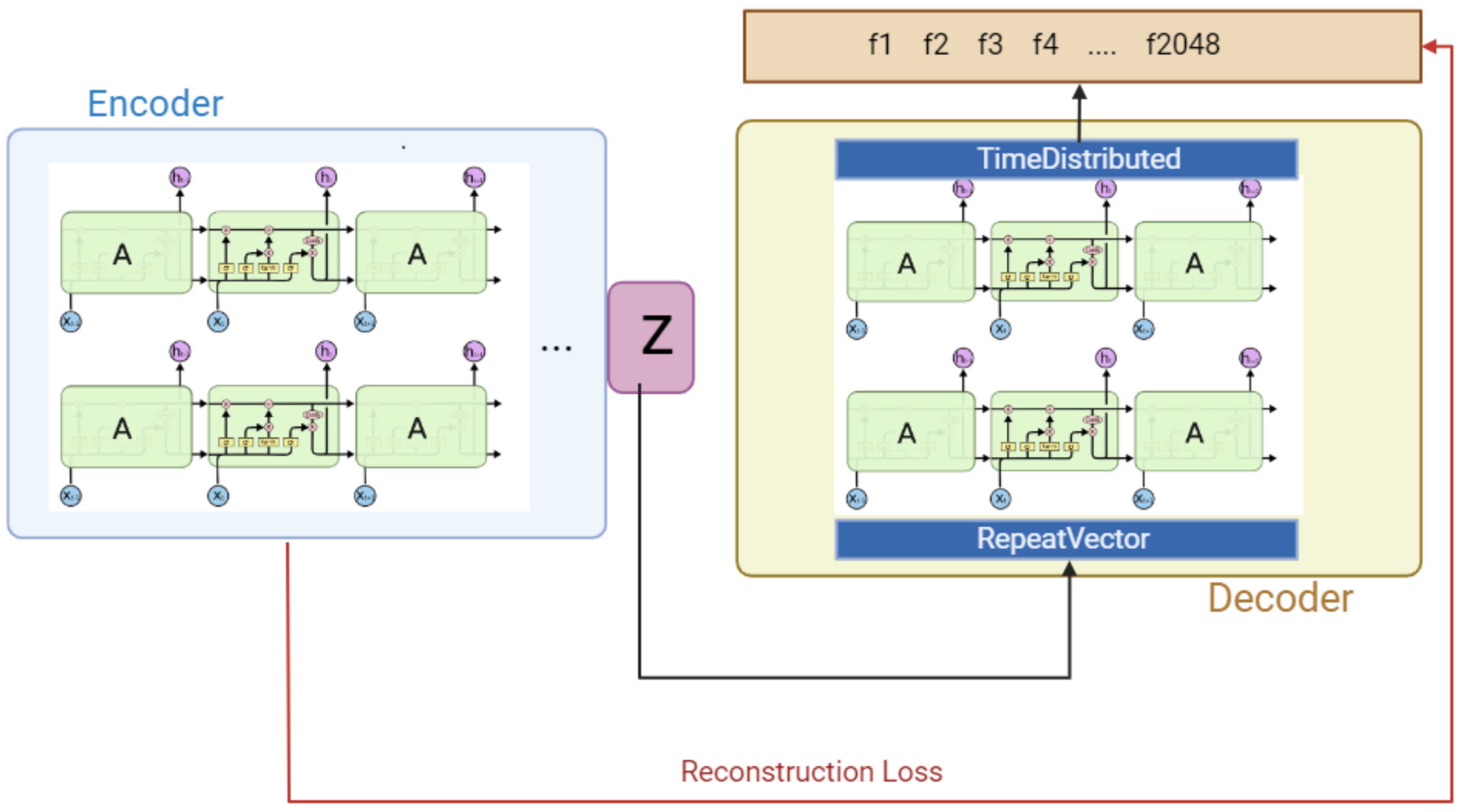
The structure of the LSTM-autoencoder is depicted in Figure 2, as follows. The encoder uses LSTM layers to capture and learn the temporal patterns inherent in time-series data. This approach takes advantage of the LSTM’s ability to retain long-term dependencies, which is critical for extracting relevant information from sequences with complex structures.These features are then transformed into a fixed-size vector Z, which represents a compressed form of the data. The decoder uses the latent vector Z generated by the encoder to reconstruct the original data. By integrating LSTM layers and time-distributed layers, the reconstructed data minimize errors when compared to the original input data. In this process, the repeat vector replicates the latent vector Z across each time step of the decoder, providing the necessary information to reconstruct the temporal patterns. The structure of the model is as shown in Table 1.
The LSTM-autoencoder model consists of an encoder and a decoder. The encoder has the same size as the input dimension, is composed of a single LSTM layer, and sets the size of the hidden state. The decoder uses the same hidden size as the encoder’s hidden state and has an output dimension that is identical to the encoder’s input dimension. It is also composed of a single LSTM layer. The combined autoencoder model uses mean squared error (MSE) as its loss function and is trained using the Adam optimizer with a specified learning rate. During training, the model is trained for a specified number of epochs, using early stopping with a patience of 3. Additionally, batch sizes are set for the train loader and validation loader. During model evaluation, the test loader is used, and the average loss value is returned to measure model performance.
The detection of noise signals in this model is based on the analysis of reconstruction errors produced by the autoencoder. When the LSTM-autoencoder reconstructs data that contain noise or anomalies, it generates high reconstruction errors, which serve as an indicator that the input data deviate from normal patterns. These anomalies appear as distinct peaks on a graph, allowing for visual identification of noise. In practical applications, when unexpected fluctuations are detected in time-series data, the model quickly identifies and classifies them as noise, distinguishing them from actual leak signals. By analyzing the difference between the predicted waveform and the actual data, anomalies in the pipeline can be accurately determined. This improves the accuracy of the leak detection system, reduces management and operational costs, and helps minimize water resource loss [15,16,17].

2.3. Signal Detection

Classifying leak data in modern water supply and sewage systems is a complex task that requires high precision to distinguish among numerous signals within the infrastructure. This classification is often facilitated by machine learning models trained to recognize patterns indicating leaks from vast amounts of time-series sensor data [18]. These patterns are characterized by anomalies in normal operating data, which may include unexpected pressure changes, flow rates, or acoustic signals that deviate from the baseline. In the proposed paradigm, integrating an ensemble model into the leak detection process is expected to significantly improve the classification accuracy. An ensemble model is a form of machine learning that combines the predictions of multiple models to enhance reliability and accuracy compared to a single-model approach. This approach leverages the strengths of different models, which together provide more robust predictions by complementing each other’s weaknesses. Ensemble models significantly enhance the accuracy of leak detection by reducing issues such as overfitting to the noise in the training data, to which individual classifiers may be vulnerable. This method enhances the reliability of pipeline management by minimizing risks and variabilities, combining domain expertise with data-driven predictions, and reducing false alarms. It addresses the inherent complexity of pipeline data and provides adaptability, allowing the system to evolve with new changes over time [19,20,21].
To implement such a system, the LSTM-autoencoder serves as an initial noise-reduction stage, effectively cleansing the data for subsequent classification processes. After the data have been filtered for noise, the classifier ensemble takes over to determine the presence of a leak. This decision is reached by aggregating the outputs of multiple classifiers, either through a voting mechanism, where the majority decision prevails, or by averaging their predictions to enhance reliability [22,23]. By implementing an ensemble model, the detection system not only improves accuracy but also enhances the robustness and reliability of leak detection by mitigating the limitations of individual models. This ensemble approach is particularly effective in addressing the complex characteristics of pipeline conditions where single-model approaches may fail. The system’s precision in identifying leaks ensures the prompt detection of even minor anomalies, reducing environmental damage from water loss. This method contributes to the improved maintenance of pipeline systems and advances pipeline monitoring technology [24].

2.4. Ensemble Model

This ensemble classifier includes a variety of machine learning models, including: RandomForestClassifier, XGBClassifier, LogisticRegression, KNeighborsClassifier, DecisionTreeClassifier, ExtraTreesClassifier, GradientBoostingClassifier, AdaBoostClassifier, SVC (Support Vector Classifier), MLPClassifier (Multi-Layer Perceptron Classifier), LGBMClassifier (LightGBM Classifier), and CatBoostClassifier.
  • RandomForestClassifier: Combines multiple decision trees trained on random subsets of data. The final output is determined by averaging the predictions of these trees, offering high accuracy and resistance to overfitting.
  • XGBClassifier: An enhanced gradient-boosting model that corrects the errors of previous models sequentially. It is known for its fast speed and high performance, especially in data science competitions.
  • LogisticRegression: A probabilistic model for binary classification, predicting the probability of a specific class by limiting results to values between 0 and 1.
  • KNeighborsClassifier: An instance-based learning algorithm that classifies data points by finding the k nearest neighbors in the dataset.
  • DecisionTreeClassifier: A tree-structured model where nodes represent decisions based on data features, and leaf nodes indicate final classification outcomes.
  • ExtraTreesClassifier: An ensemble learning technique that is similar to RandomForest but uses more trees and introduces additional randomness in the decision splits.
  • GradientBoostingClassifier: Sequentially improves weak predictive models by focusing on reducing errors and minimizing the loss function during training.
  • AdaBoostClassifier: Combines weak learners into a strong learner by sequentially improving models, giving higher weights to misclassified instances.
  • SVC (Support Vector Classifier): A support vector machine-based classifier that identifies the decision boundary with the maximum margin between classes.
  • MLPClassifier (Multi-Layer Perceptron Classifier): A neural network-based classifier with one or more hidden layers, which is capable of learning complex patterns in data.
  • LGBMClassifier (LightGBM Classifier): A lightweight gradient boosting machine known for its efficiency in handling large-scale data and fast learning speeds.
  • CatBoostClassifier: A gradient boosting classifier that excels in handling and converting categorical variables automatically.
These classifiers undergo a grid search for hyperparameter optimization. They learn different aspects of the data and contribute to the final prediction through a voting system. This ensemble approach provides more robust and accurate classification performance than any single model, ensuring the accurate classification of data into actual leak signals and normal signals [25,26,27].

3. LSTM-Autoencoder-Based Noise Signal Detection

3.1. System Framework

The proposed framework is structured into three distinct processes, each designed to handle specific tasks in the processing pipeline for time-series data. These processes include noise signal estimation, noise attenuation, and final data classification, all working together to ensure accurate leak detection.
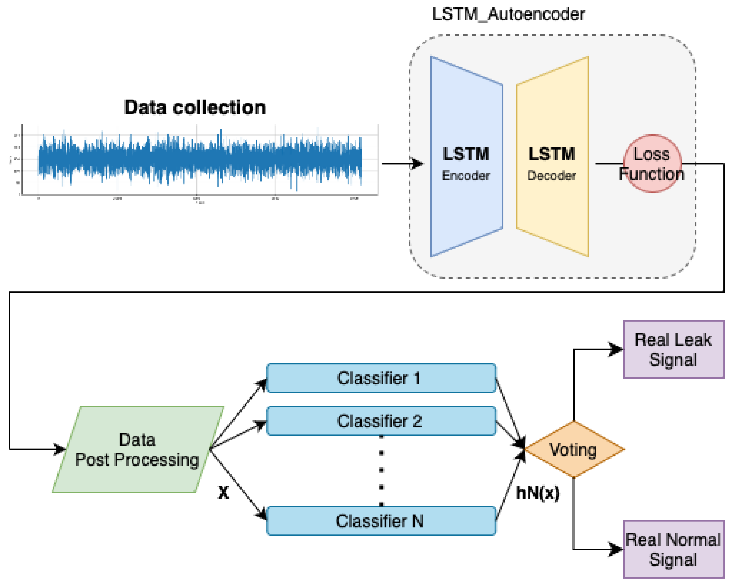
The structure of the proposed framework is depicted in Figure 3, as follows.
  • Noise Signal Estimation: This process is the initial process after collecting time-series data. In the LSTM-autoencoder, the key features of the time-series data are learned and condensed into a low-dimensional representation, denoted as Z. Noise is detected by comparing this compressed representation with the original time-series data; significant discrepancies indicate the presence of noise. This process allows for the identification of anomaly causes in the data and minimizes the impact of noise.
  • Noise Signal Attenuation: This process removes the noise identified in the noise signal estimation process. It detects parts with significant deviations compared to the actual data and focuses on noise reduction in areas with a high proportion of anomalies. This includes reducing outliers while optimizing the overall data’s loss value. After processing, the noise-reduced data are passed to the next process, the ensemble model.
  • Normal and Leak Data Classification: In the final process, the ensemble model, which combines multiple classifiers (Classifier 1 to Classifier N), performs a final prediction. Each classifier learns different aspects of the data, and their results are reflected in the final decision through voting. The combined ensemble model provides a more robust and accurate classification performance than a single model. As a result, the noise-reduced data are accurately classified into ’Real Leak Signal’ and ’Real Normal Signal’.
This framework provides a powerful tool for processing real-time or large-scale time-series data, effectively reducing noise, and quickly detecting and responding to issues through accurate classification.

3.2. Loss Function

The noise signal estimation layer plays a critical role in the initial processing of the collected time-series data, where it conducts a preliminary analysis aimed at detecting and quantifying noise within the dataset. This layer identifies data segments that significantly deviate from expected patterns, marking them as potential noise. In this study, approximately 30% of the data collected from the installation point to the present are selected and used as the training dataset. The selected data are fed into an autoencoder model integrated with LSTM, which is designed to learn the complex dynamic patterns of time-series data. After training the model, new data collected in the actual operating environment are reconstructed through the structure. The difference between the reconstructed data and the actual collected data is calculated to detect noise. If the reconstruction error exceeds a threshold, the data point is considered to deviate from the expected normal flow and is classified as noise. The threshold can be adjusted based on the distribution of the data and the characteristics of the noise. In this study, the optimal threshold is derived through cross-validation. Through this process, the model can identify noise in real-time, providing critical foundational data for subsequent processing stages such as noise attenuation and data classification within the overall framework. To evaluate the performance of the noise signal estimation layer, experiments were conducted using real time-series data that includes various types of noise, demonstrating the model’s effectiveness.
This section describes the configuration and optimization method of the loss function related to the noise-attenuation process derived from the noise signal estimation layer. The primary goal of the noise signal attenuation layer is to minimize the impact of the data segments that contain the identified noise. A systematic approach using reconstruction error is adopted to achieve this. The noise signal attenuation process focuses on segments where the reconstruction error exceeds a specific threshold, and it gradually reduces the difference from the actual data in those segments. This adjustment is made by progressively decreasing the parts of the actual data corresponding to the noise.
The loss function is defined as shown in Equation (1):
L ( x , x ^ ) = i = 1 N x i x ^ i
Here, x represents the actual data, x ^ is the data reconstructed by the autoencoder, and N is the total number of data samples. The goal is to minimize the sum of the absolute errors for each i-th data point [28,29]. The threshold is determined based on the outlier values of the reconstruction error. The outlier value is selected from among the values corresponding to 95% to 100% of the data, and this process is carried out while gradually decreasing at an interval of one-thousandth. The threshold at each step is determined as shown in Equation (2):
θ p = Quantile ( L ( x , x ^ ) , p )
Here, θ p represents the threshold corresponding to the p-th percentile [30,31]. The optimal threshold is selected to minimize the total loss value for the entire dataset while maximizing the noise attenuation effect for the outlier segments. In this study, we observed changes in the loss function as the threshold θ is varied, and through this process, we selected the optimal θ value. To evaluate the performance of this layer, various experiments were conducted on the loss function. These served as crucial indicators for assessing the impact of the noise-attenuation process on the actual data.

3.3. Voting

After reducing noise using the LSTM-autoencoder, frequency characteristics were extracted through fast Fourier transform (FFT) preprocessing. This step is crucial, as it highlights essential features of the signal that may not be clear in the time domain.
X ( k ) = n = 0 N 1 x ( n ) e i 2 π k n / N
Here, X ( k ) represents the k component in the frequency domain representation, x ( n ) is the n component of the time domain signal, N is the total number of samples, and e is the base of the natural logarithm. By mapping the time domain data to the frequency domain, the FFT reveals patterns and trends within the frequency band. The detected anomalies allow for the visual confirmation and precise classification of signals suspected of leakage, enabling continuous monitoring of the system.
This process allows for the identification of patterns and trends within the frequency band, which is crucial for detecting suspected anomalies within the signal. Through this frequency analysis, suspected leaks can be visually confirmed, accurately classified, and continuously monitored within the system. This post-processing step sets the stage for more detailed analysis, providing refined and frequency-enhanced data as input for subsequent ensemble classification [32,33,34,35]. In the classification stage, a classifier ensemble using various machine learning algorithms or parameter settings is applied. Each classifier C i within the ensemble can be modeled as follows:
y = C i ( x ; θ i )
Here, y represents the predicted value, C i is the i classifier, x is the input data, and θ i is the parameter of the i classifier.
Decision trees, support vector machines, and neural networks are trained on the frequency domain data to distinguish between normal operational noise and leakage characteristics. This step ensures that the complex features of the leakage are captured by the collective ability of the classifiers [36]. In the voting stage, the predictions from each classifier are aggregated to reach a final decision. The aggregation can be performed in the form of a weighted sum, where the weight w i represents the reliability of the i classifier:
Y final = i = 1 n w i · y i
Here, Y final is the aggregated output, n is the number of classifiers, and y i represents the prediction of the i classifier. The weight coefficient W i represents the reliability of each classifier with weights assigned based on the error rate of each classifier. The lower the error rate, the higher the weight assigned. If the error rate of classifier i is E r r j , the weight is determined accordingly.
w i = 1 E r r i j = 1 n ( 1 E r r j )
This consensus-based mechanism is designed to reduce the bias or errors of individual classifiers, thereby enhancing the overall system’s reliability. A model that reaches a consensus through majority voting signals potential leakage and triggers an alert for further investigation or immediate action according to the established operational protocols [37,38].

4. Experimental Application

4.1. Experimental Environment

Table 2 shows the experimental environment of the hardware and software used to conduct the study. The hardware configuration included an Intel Xeon Silver 4216 CPU @ 2.10 GHz processor (Intel, Santa Clara, CA, USA) and four NVIDIA RTX A5000 graphics cards (NVIDIA, Santa Clara, CA, USA). The operating system used in the software is Ubuntu 18.04.6 LTS. We used Python 3.10.9 as a programming language, which is widely used in the field of data analysis and machine learning. We also utilized TensorFlow 2.11.0, an open-source machine learning framework, to develop and run our model. TensorFlow provides a variety of libraries related to deep learning model development.

4.2. Dataset and Data Preprocessing

To detect leaks in water supply pipelines, battery-powered IoT sensor modules are deployed, utilizing Industrial Internet of Things (IIoT) sensor networks and LTE-M network technology. These sensors are designed to detect vibrations and transmit the collected time-series data to a cloud system at specified intervals via the LTE-M network.
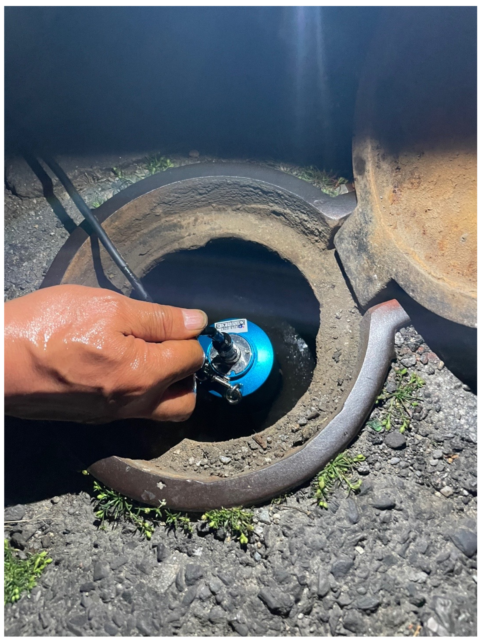
Field surveys are conducted to determine the optimal location for gate valve installations, taking into account factors such as accessibility, environmental conditions, and signal strength. As shown in Figure 4, an antenna is connected to the sensor to facilitate smooth communication with the cloud system through the LTE-M network. The connection status is checked to ensure that the signal strength is strong enough, thereby ensuring stable data transmission.
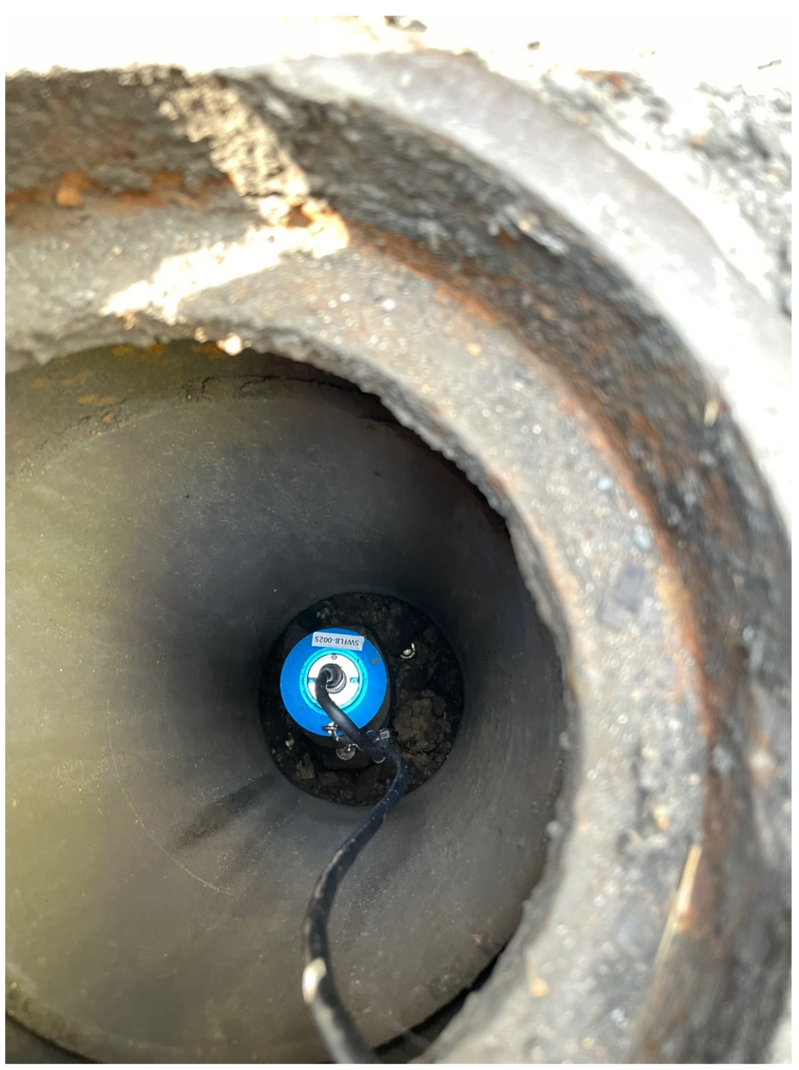
As illustrated in Figure 5, the sensor, equipped with the connected antenna, is attached to the pipeline inside the gate valve. The sensor is securely mounted so that its center was in close contact with the pipeline, enabling the accurate measurement of vibrations transmitted through the pipeline. The antenna is firmly affixed to the valve to enhance communication stability and was positioned close to the ground to optimize the communication rate with the server.
As shown in Figure 6, the antenna attached to the sensor is installed near the ground to improve the communication rate with the server. The sensor collects vibration data according to a pre-set period and method, with the collected data being transmitted to the cloud system through the LTE-M network. The transmission interval is adjustable, typically ranging from a few minutes to several hours. The transmitted data are stored in the cloud system for real-time monitoring and analysis [39].
The experiment utilized sensor data provided by the S Company, including instances where leaks were detected in actual water pipelines. As depicted in Figure 7, data collection and processing were thoroughly conducted. This dataset comprises a total of 19,697 leak cases and 20,000 normal cases. The data were meticulously gathered, encompassing various variables such as the pipeline material at the leak point, the time of the leak, the type of leak, and the location of the sensors. This comprehensive dataset reflects diverse environmental conditions and scenarios, enabling an effective evaluation of the leak detection algorithm’s performance.
In the dataset, sensor data are listed in chronological order. The oldest 30% of the data was used to train the model, during which outliers were removed to ensure that the noise signal estimation model could clearly classify noise in the data that is not part of the training dataset. To remove noise from the dataset, a combination of an autoencoder and LSTM models is employed. The autoencoder extracts the main features of the time-series data, while the LSTM learns the dynamic patterns of the time-series data based on these features. This process allows the model to estimate noise signals in the time-series data and analyze reconstruction errors to identify and filter out noise [39].
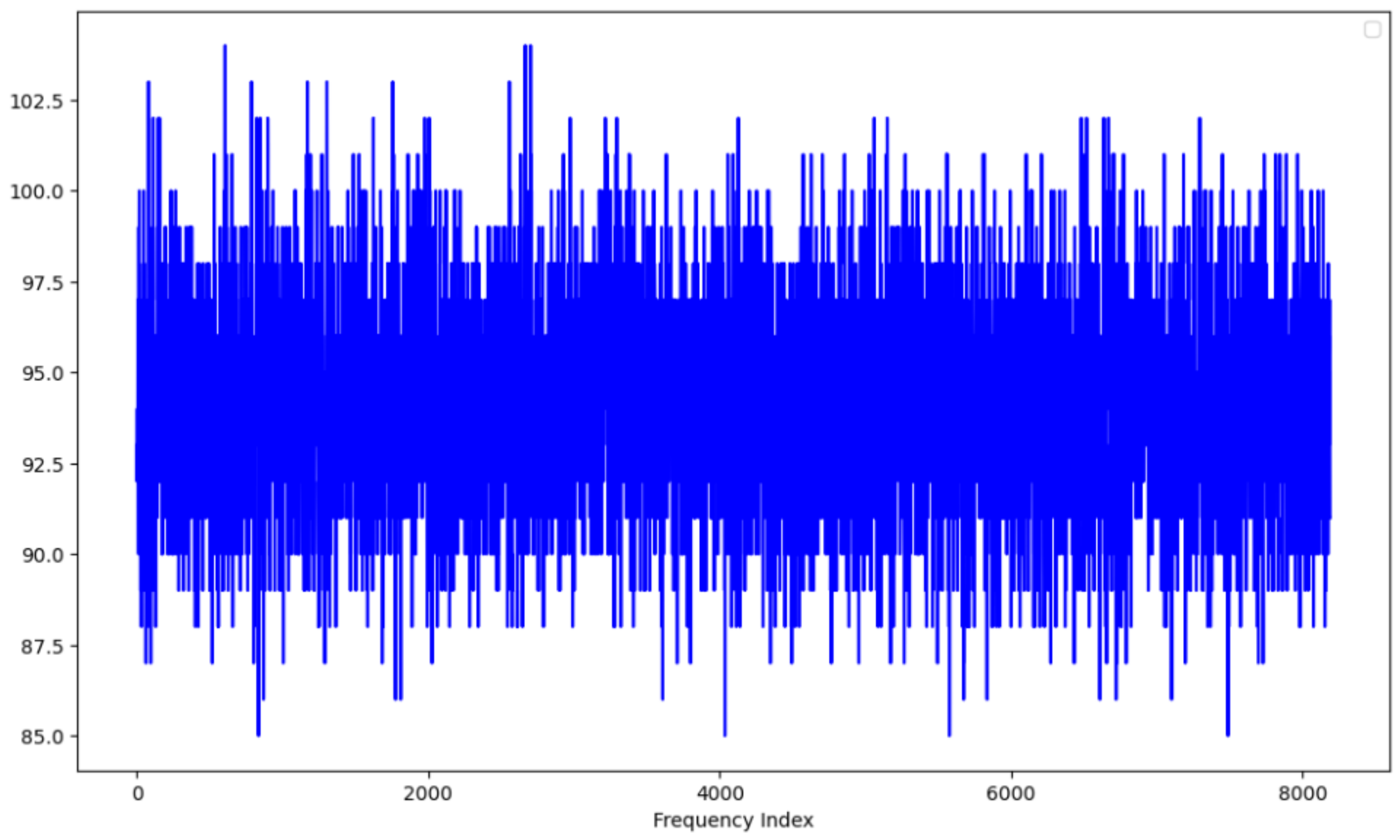
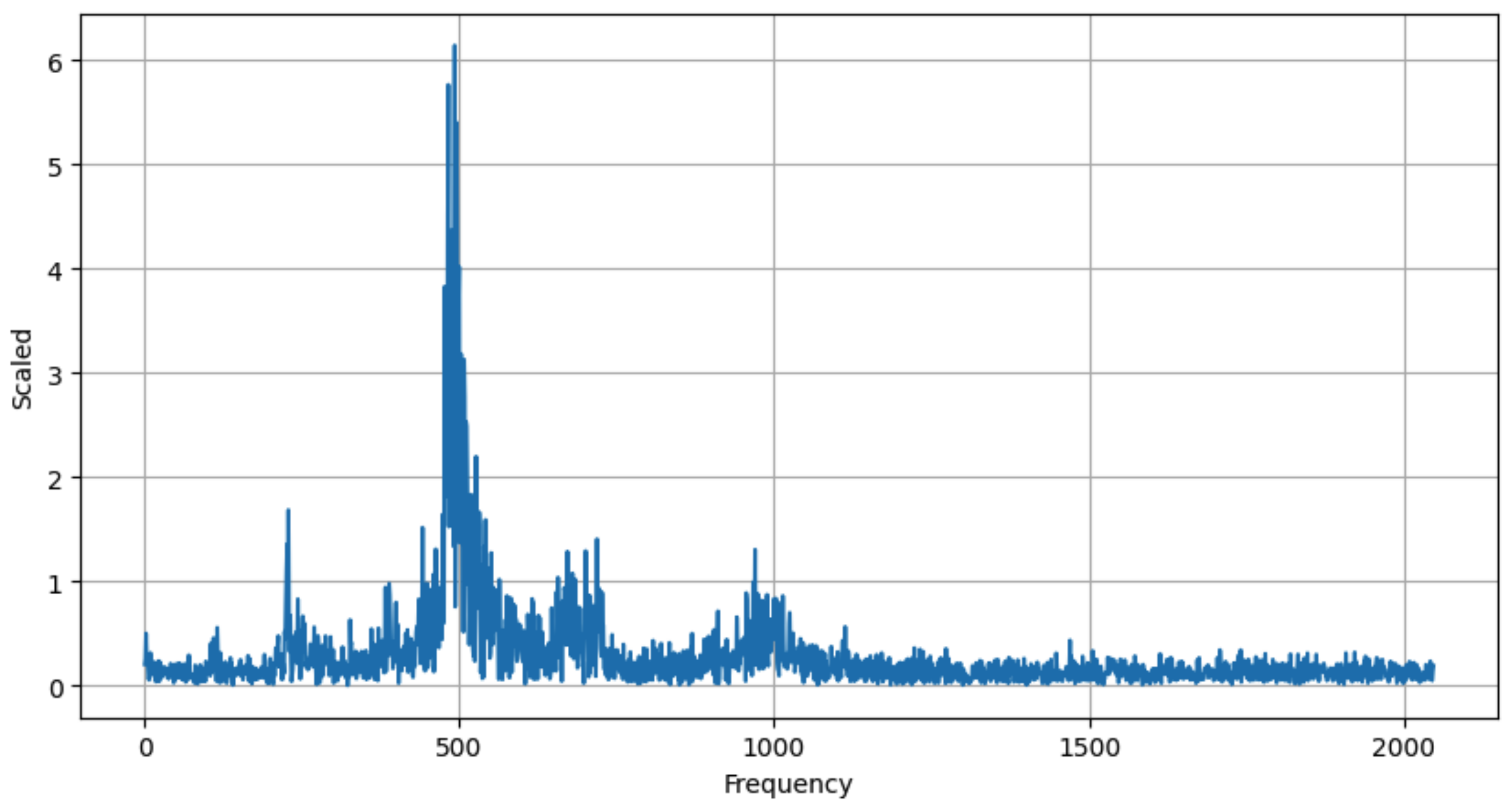
Figure 8 and Figure 9 illustrate the frequency analysis of leakage data, showcasing the process of detecting leaks through FFT analysis. Figure 8 represents the time-series data of the leakage, where the x-axis indicates the number of samples over time, and the y-axis displays the range of measured values. By contrast, Figure 9 presents the frequency data obtained through the FFT, with the x-axis representing frequency ( H z ) and the y-axis showing the amplitude of the frequency components. The FFT graph in Figure 9 reveals prominent peaks, particularly in the lower frequency range, indicating the key frequencies where the leakage signal is most significant. This contrast between the time-domain and frequency-domain representations highlights the importance of frequency analysis in identifying the characteristics of the leakage. However, a significant challenge arises when noise is present in the data. While frequency analysis can help identify leakage signals, distinguishing between the actual leakage signal and noise becomes difficult when both are mixed. This can lead to inaccuracies in diagnosing the leakage. To address this issue, the proposed architecture aims to extract the pure leakage signal by effectively removing noise from the data. This approach ensures that the analysis focuses solely on the true characteristics of the leakage, leading to more accurate detection and monitoring.
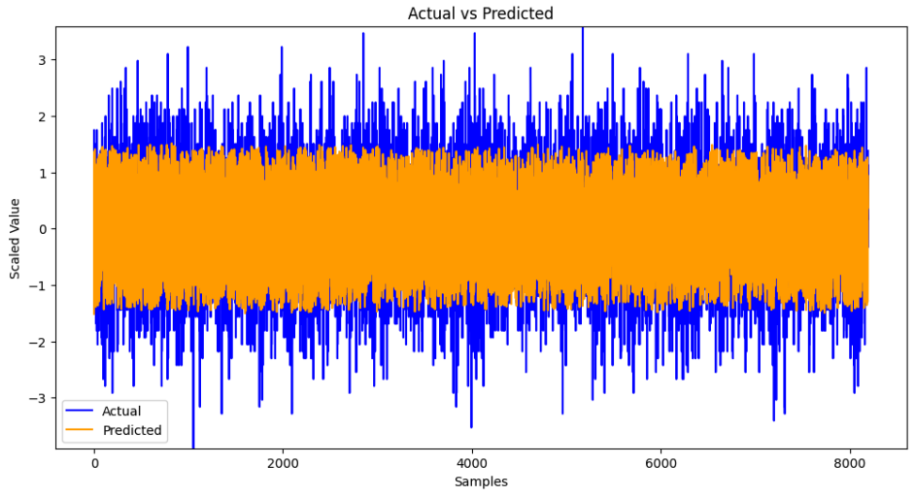
The model infers the waveform at time points not in the training data using the remaining 70% of the dataset. Figure 10 shows the difference between actual and predicted waveforms at noise-free time points. The x-axis represents the number of collected samples, while the y-axis shows the magnitude of the actual collected data. When the pipeline operates normally, the difference between the actual time series data and the predicted data is minimal, indicating consistency in vibration data during normal system operation. The difference between actual values (blue) and predicted values (orange) is generally small, suggesting that the prediction model closely follows the pattern of the actual data. The data scale ranges between −3 and 3, indicating proper scaling of the data. The orange area represents the range of predicted values, which mostly encompasses the variation range of the actual values, indicating a high accuracy of the model for noise-free data. The small difference between actual and predicted data during normal system operation implies high reliability, facilitating easier detection of anomalies like leaks.
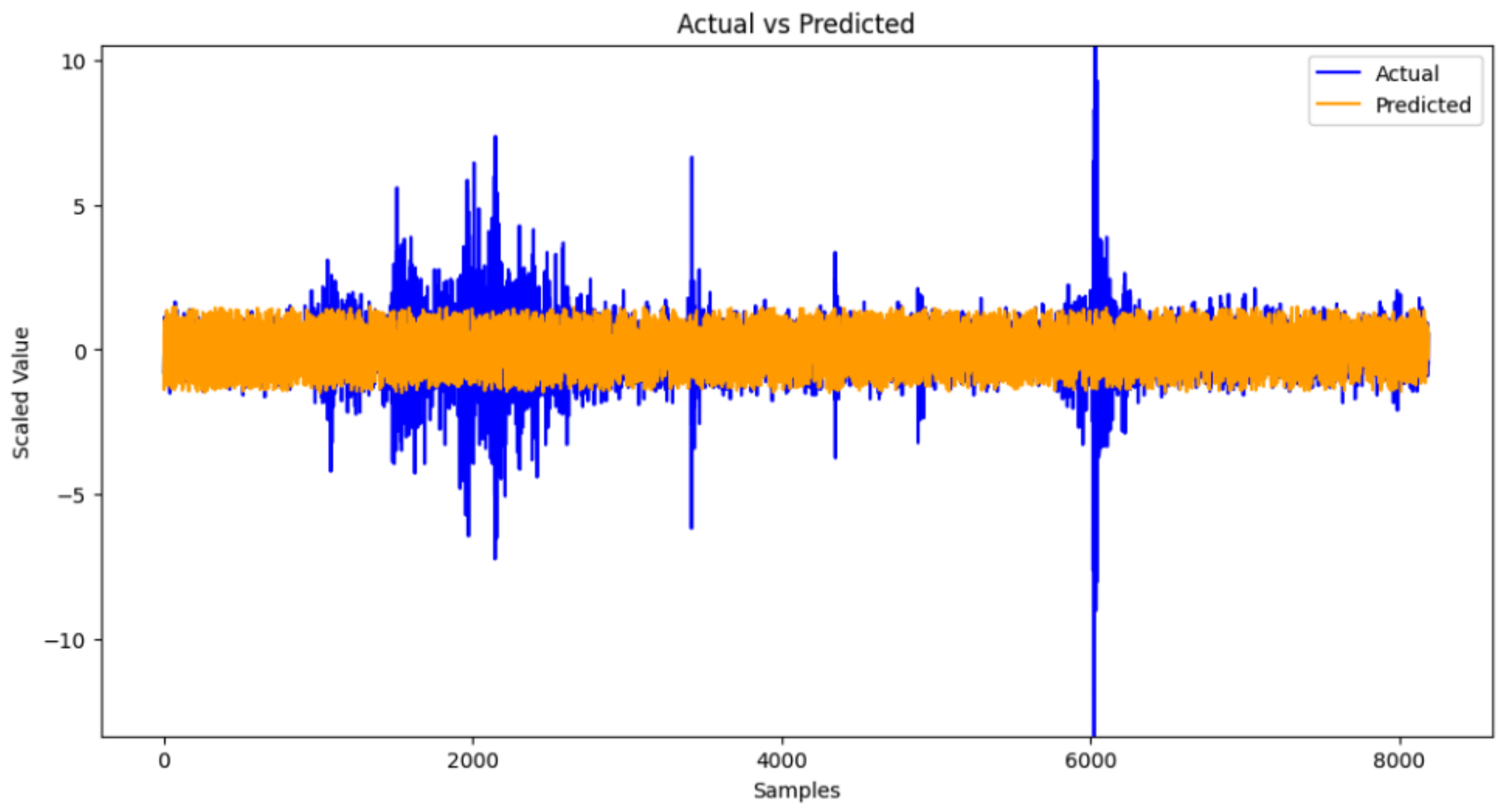
Figure 11 shows the difference between actual and predicted waveforms at noisy time points. This figure illustrates the difference between actual and predicted values for data with noise. The x-axis represents the number of collected samples, while the y-axis shows the magnitude of the actual collected data. When noise is present, the difference between actual data (blue) and predicted data (orange) becomes larger, especially in segments with significant noise. This discrepancy is crucial for assessing the model’s capability to handle noisy data. The orange area represents the range of predicted values, which mostly encompasses the variation range of the actual values, indicating that the model still captures the fundamental pattern of the data even with noise. However, as noise increases, the difference between predicted and actual values tends to grow. In particular, in some segments, the predicted values fail to follow the large fluctuations of the actual values, indicating the negative impact of noise on the model’s prediction performance.
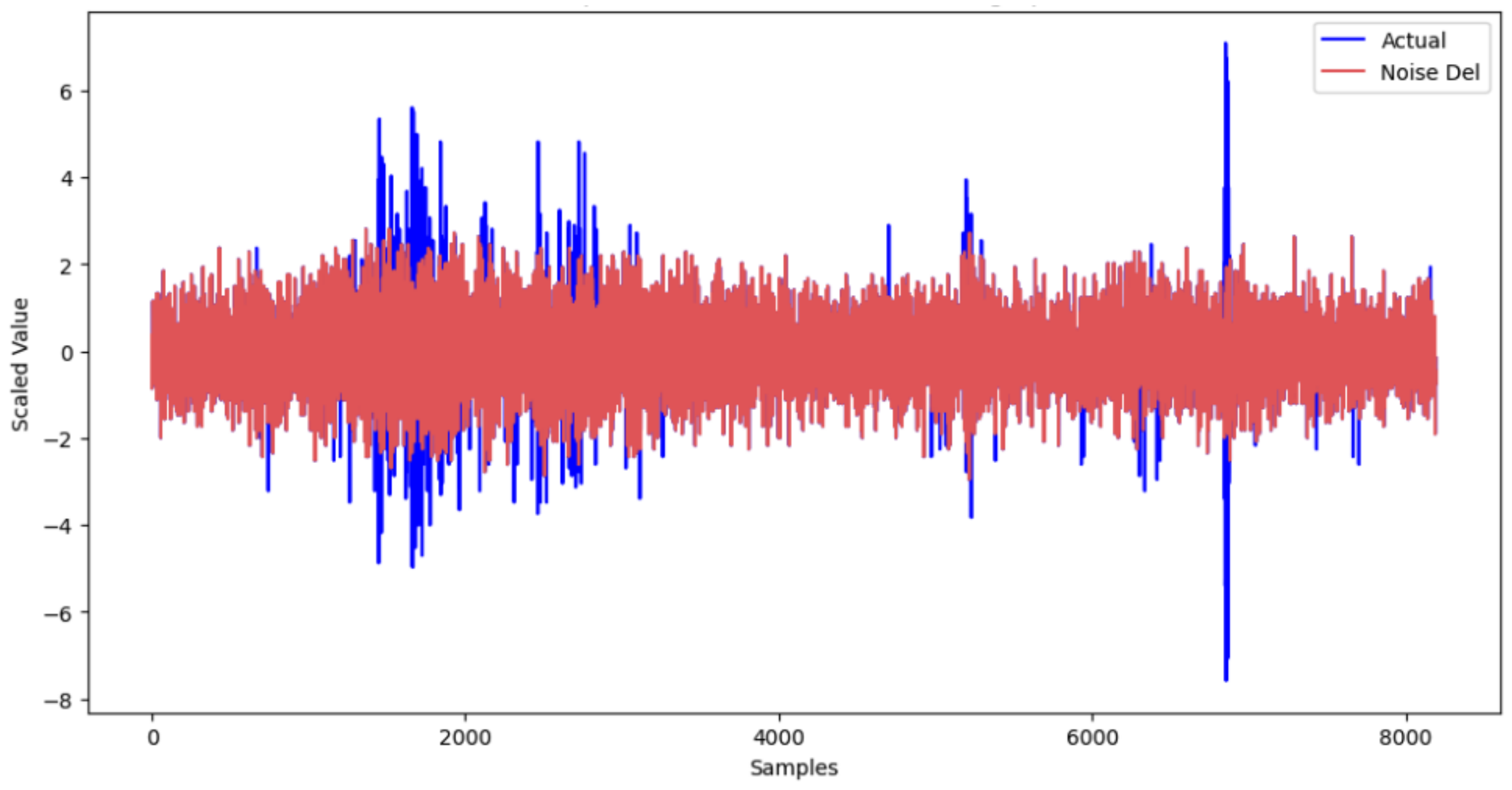
In Figure 12, the x-axis represents the number of collected samples, while the y-axis shows the magnitude of the actual collected data. This figure compares the flow of actual and reconstructed data for samples with noise, showing noise attenuation for these samples. The pink graph represents the noise-attenuated data. The noise-attenuation process refines the data to clarify the original useful signal. The pink graph, showing noise-attenuated data, reveals the vibration pattern of the actual data more clearly, which is crucial for improving the accuracy of the leak detection system. After noise attenuation, the pink graph shows reduced differences between actual and predicted values, allowing the model to predict data patterns more accurately. This enhances the system’s performance in noisy environments. As shown in Figure 12, data identified with noise are attenuated, focusing on sections with large variations to minimize the impact of noise.
After noise attenuation, the data undergo FFT preprocessing, which is widely used in vibration signal analysis to extract frequency characteristics. This step highlights important features of the signal that are not apparent in the time-domain data and are crucial for identifying patterns and trends in the frequency domain. Through frequency analysis, suspicious portions of the signal can be identified, visually confirmed, and accurately classified as suspected leaks, allowing the continuous monitoring of the system’s condition. This process lays the foundation for subsequent analysis. The extracted frequency data are then fed into an ensemble classifier. This ensemble classifier is a system composed of various integrated machine learning models that distinguishes actual leakage events from normal conditions with high accuracy for the given dataset. Each model is independently trained to analyze data from different aspects, and their predictive results are combined to determine the final leakage status. In this process, the ensemble model overcomes the limitations of individual models, minimizes error possibilities based on their strengths, and ultimately provides more reliable leak detection results. This approach enables more sophisticated and efficient leak detection methods for water supply and drainage systems, allowing for quicker and more accurate responses to potential issues.

4.3. Evaluation Metrics

Several evaluation metrics are commonly used to assess the performance of classification machine learning models. Some of the most popular metrics are as follows:
Accuracy: The most intuitive and simplest metric, measuring the ratio of correctly predicted instances to the total number of instances. It gives a quick overview of how well the model performs.
Accuracy = T r u e P o s i t i v e T r u e P o s i t i v e + F a l s e P o s i t i v e + T r u e N e g a t i v e + F a l s e N e g a t i v e
Recall: Measures the ratio of correctly predicted positive instances out of all actual positive instances in the data. It is useful when the cost of false negatives is high. It shows how well the model captures actual positive cases.
Recall / Sensitivity = T r u e P o s i t i v e T r u e P o s i t i v e + F a l s e N e g a t i v e
Precision: Measures the ratio of correctly predicted positive instances. It is useful when the cost of false positives is high. This indicates how well the model ensures the correctness of positive outcomes.
Precision = T r u e P o s i t i v e T r u e P o s i t i v e + F a l s e P o s i t i v e
F1 Score: The harmonic mean of precision and recall, providing a balanced metric that considers both false positives and false negatives. It offers a comprehensive evaluation of the model’s performance on both fronts [40,41].
F 1 - Score = 2 · Sensitivity · Precision Precision + Sensitivity
Area under the curve (AUC) represents the area under the receiver operating characteristic (ROC) curve. The ROC curve is a tool for visualizing the performance of a binary classifier, displaying the true positive rate (TPR) and the false positive rate (FPR) at various classification thresholds. TPR is the same as recall and indicates the ratio of actual positive cases correctly predicted as positive. FPR indicates the ratio of actual negative cases incorrectly classified as positive.
TPR = T r u e P o s i t i v e T r u e P o s i t i v e + F a l s e N e g a t i v e
FPR = F a l s e P o s i t i v e T r u e N e g a t i v e + F a l s e P o s i t i v e
The AUC value ranges between 0 and 1. A perfect classifier has an AUC of 1, while completely random guessing has an AUC of 0.5. Therefore, the higher the AUC value above 0.5, the better the model’s performance. AUC is a metric that fairly evaluates the performance of a model even with imbalanced datasets. For example, when the sample size of one class is significantly larger than the other, AUC still reflects this imbalance well. AUC comprehensively evaluates the performance change when the model’s predicted probability threshold is altered. This allows for an overall assessment of the model’s performance without depending on a specific threshold.

5. Results and Discussion

5.1. Results

The architecture proposed in this study represents a significant advancement in water pipeline leakage detection technology, introducing an innovative combination of machine learning models and advanced signal processing techniques to address challenges in this field. Compared to existing methods, the proposed framework offers several key improvements, which are highlighted in this section.
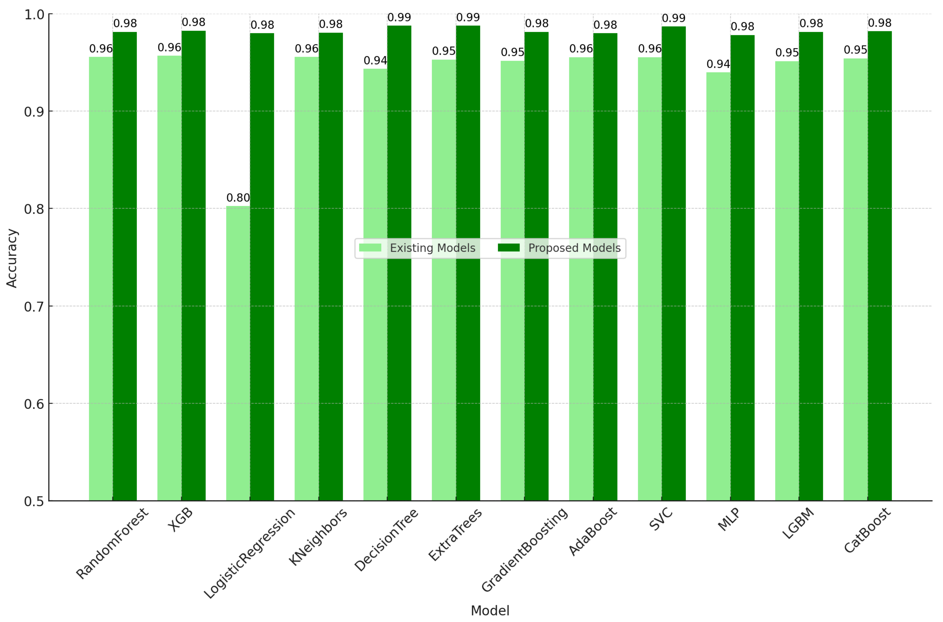
Figure 13 shows a comparison of the accuracy of the existing and proposed architectures for each model. The proposed model shows improvement in accuracy across all models, particularly in the RandomForest and XGB models.
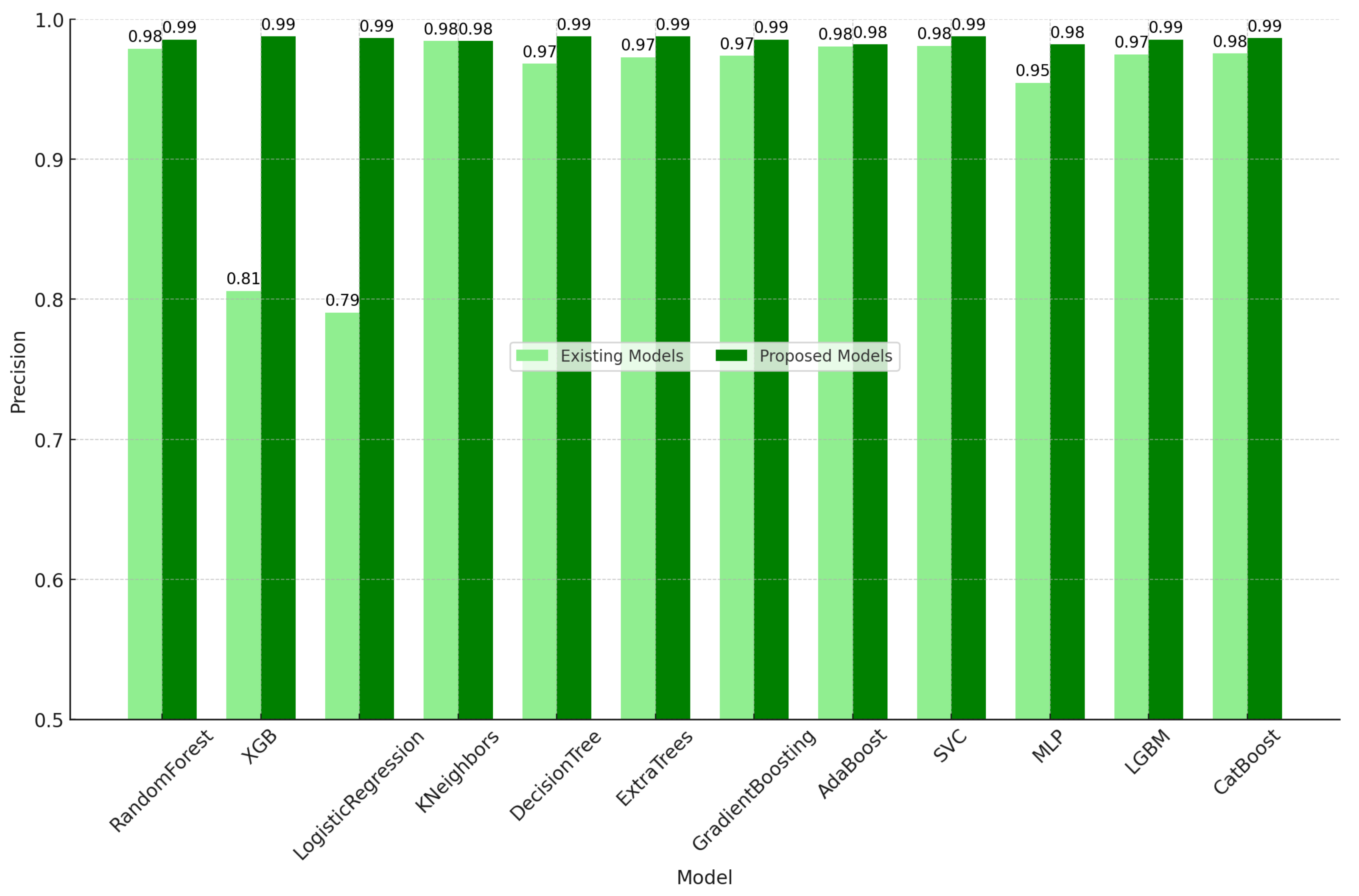
Figure 14 shows a comparison of the precision of the existing and proposed architectures for each model. In terms of precision, the proposed model also outperforms the existing model, indicating that the model makes more accurate predictions with fewer false positives.
Figure 15 shows a comparison of the recall of the existing and proposed architectures for each model. The recall comparison results show that the proposed model records higher recall than the existing model, indicating an improved ability to capture true positive cases.
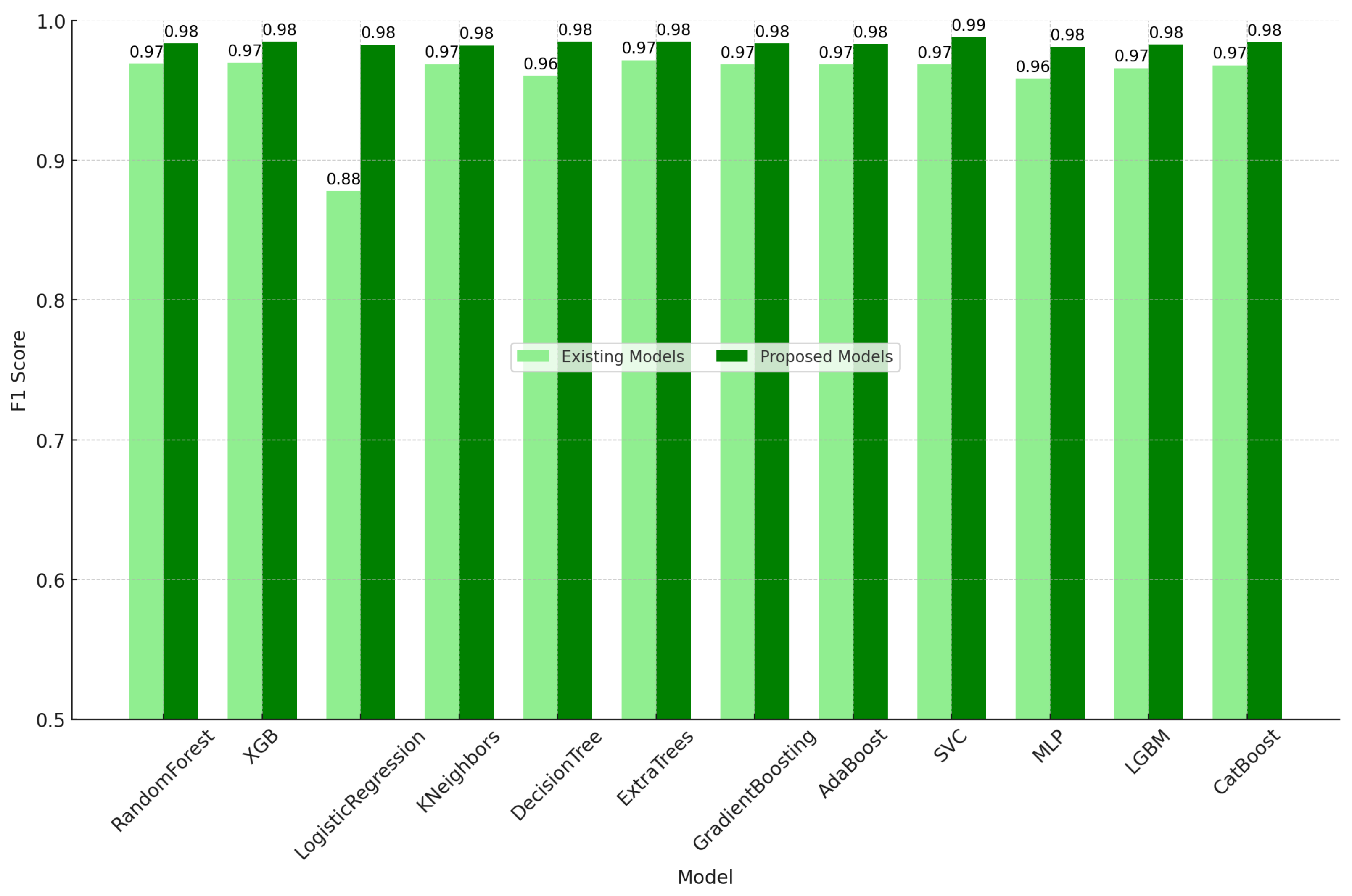
Figure 16 shows a comparison of the F1 scores of the existing and proposed architectures for each model. The F1 score, which represents the harmonic mean of precision and recall, also shows that the proposed model outperforms the existing model, indicating a balanced improvement in overall performance.
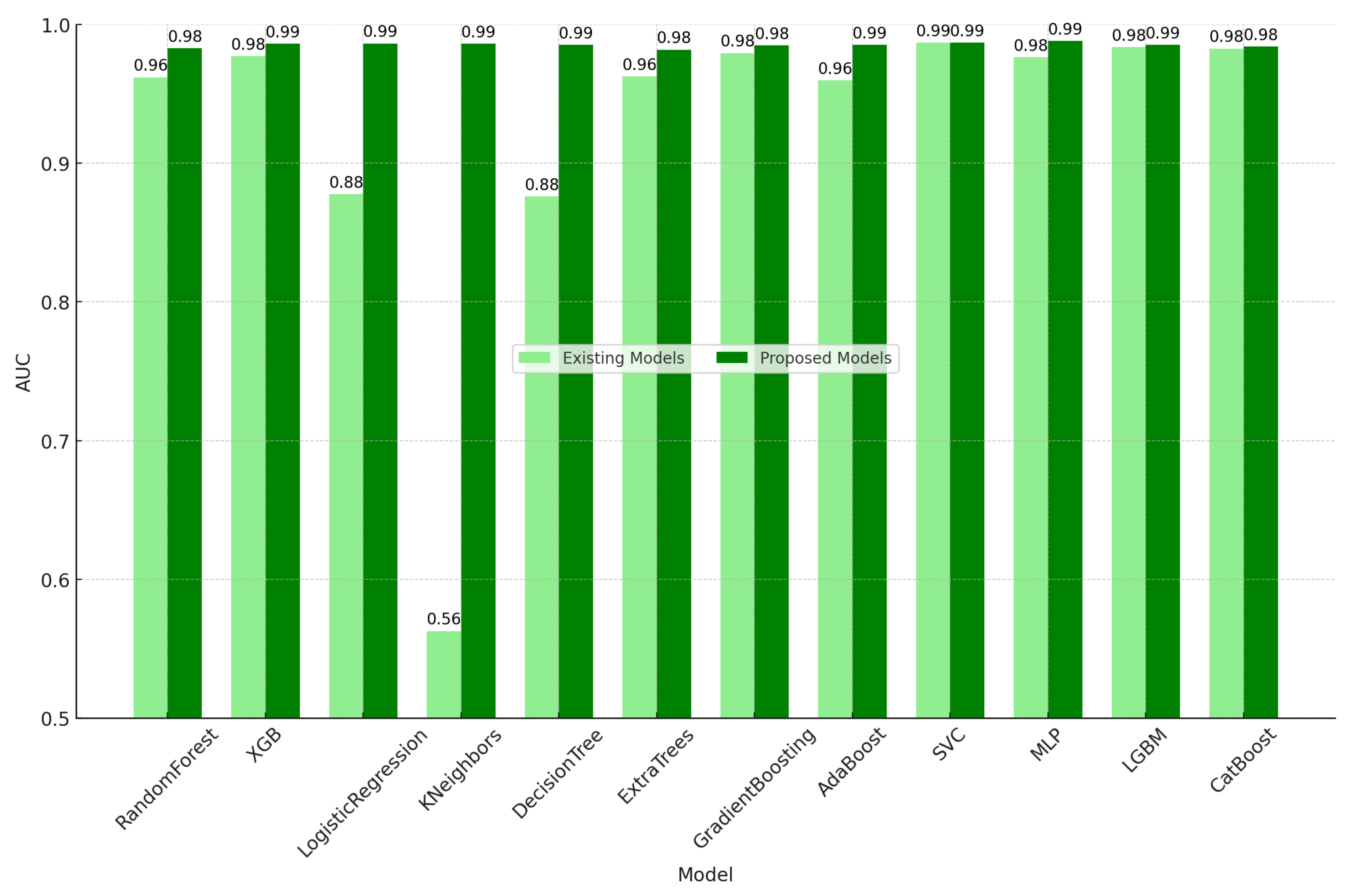
Figure 17 compares the AUC scores before and after applying the proposed architecture, showing an increase in AUC scores for most models, thus validating the effectiveness of the proposed approach. The following table presents the performance evaluation metrics of the models before and after applying the proposed architecture to 12 different models.
Table 3 compares the performance of the ensemble model without noise removal and the proposed architecture. When using existing machine learning models, noise signals included in the data sometimes misled the models, causing incorrect learning as if the noise was an actual leak signal. This often led to incorrect predictions. By contrast, the proposed architecture effectively removes noise through a noise-attenuation process, allowing the models to focus on actual leak signals. This process emphasizes the important features of the signals, improves the data quality, and enhances the overall performance of the classifiers. The noise-attenuated data provide clearer vibration patterns, which serve as critical information for the models to recognize leak signals. Additionally, the proposed architecture uses an ensemble classifier that combines multiple models, enabling a more accurate distinction between leaks and normal states.
After applying the proposed architecture, the performance of most models improved noticeably. For instance, the accuracy of RandomForest increased from 0.9558 to 0.9814, and for XGB, the accuracy increased from 0.957 to 0.9827, with recall rising from 0.9593 to 0.9877. The Logistic Regression model showed a significant improvement in accuracy from 0.8025 to 0.9801. These enhancements indicate that the proposed architecture is highly effective in improving the accuracy and reliability of leak detection.

5.2. Discussion

Existing leak detection methodologies often struggle with accurately identifying leaks in real-world environments due to noisy sensor data, complex pipeline conditions, and aging infrastructure. Traditional approaches typically rely on statistical methods or basic machine learning models, which can be prone to errors in noisy or variable data. These methods frequently misclassify normal conditions as leaks or fail to detect subtle signs of leakage, leading to false alarms or undetected water loss. By contrast, the proposed architecture utilizes a combination of LSTM-autoencoders and ensemble learning models to address these challenges. By incorporating advanced noise signal estimation, damping, and FFT preprocessing, this approach is capable of filtering out noise more effectively, leading to superior accuracy in leak detection. The integration of ensemble models ensures robust performance across diverse data characteristics, further enhancing the reliability of the system. This is particularly crucial in real-time monitoring, where accurate detection and quick response are essential for preventing water loss and minimizing infrastructure damage.
The experimental results demonstrate that the proposed system outperforms traditional models in several critical metrics, such as accuracy, precision, recall, and F1 score. For example, the RandomForest classifier’s accuracy improved from 95.58% to 98.14%, while the F1 score increased from 96.9% to 98.38%. Similar improvements were observed across other classifiers, including XGB, CatBoost, and Logistic Regression, showcasing the effectiveness of the proposed noise-attenuation and ensemble modeling techniques. The proposed architecture offers several key advantages that make it highly effective for water pipeline leakage detection. First, the system demonstrates improved accuracy and precision, largely due to its advanced noise reduction process. By filtering out irrelevant signals, the architecture is able to focus on meaningful data, which significantly reduces false alarms and enhances the overall detection precision. Additionally, the use of an LSTM-autoencoder enables the system to detect even subtle leakage signals, leading to an increase in recall. This capability ensures that more leakage events are captured, improving the overall leak detection efficiency. The architecture also exhibits strong robustness against noisy data, which is critical in real-world environments where sensor data are often contaminated by external factors or equipment issues. The system effectively filters out noise, ensuring accurate classification even in challenging conditions. Finally, the adaptability of the system to diverse conditions is a major strength. Through ensemble learning, the architecture is capable of handling various pipeline conditions and data characteristics, making it highly versatile and applicable in a wide range of environments. This flexibility ensures that the system can be effectively used in different scenarios without sacrificing performance.
Building on these results, future research will focus on quantifying leak volumes through frequency analysis and investigating the correlation between signal anomalies and actual water loss. Additionally, the potential for applying the proposed approach to other types of infrastructure systems and data will be explored, aiming to develop a universal solution for leak detection and monitoring across various environments. Continuous research will be conducted to further refine the model’s predictive power, ensuring its practical utility in public utility management.

6. Conclusions

The results of this study demonstrate a significant advancement in the field of water pipeline leak detection. By integrating LSTM-autoencoder with ensemble machine learning methods, the proposed architecture effectively addresses the limitations of existing detection systems. The combination of noise estimation, attenuation, and FFT preprocessing techniques enables the model to accurately differentiate between noise and actual leakage signals, improving both sensitivity and precision in real-time monitoring. The use of ensemble classifiers further enhances the robustness and reliability of leak detection by leveraging multiple machine learning algorithms, ensuring higher predictive accuracy. The proposed framework was validated through comprehensive experiments in various environmental conditions, showing significant improvements in detection accuracy, resource conservation, and cost efficiency. Overall, this study sets a new benchmark for machine learning-based leak detection systems and demonstrates the practical utility of the proposed architecture. The findings not only enhance the detection of water pipeline leaks but also open opportunities for applying this methodology to other time-series data analysis scenarios, making it a versatile tool for infrastructure management. Future research will focus on expanding the applicability of the model and further refining its predictive capabilities.

Author Contributions

Conceptualization, Y.S.; methodology, Y.S.; software, K.Y.N.; validation, Y.S.; formal analysis, Y.S.; investigation, E.J.K. and S.E.K.; resources, H.G.C.; data curation, Y.S.; writing—original draft preparation, Y.S.; writing—review and editing, K.Y.N.; visualization, Y.S.; supervision, J.J.; project administration, J.J. All authors have read and agreed to the published version of the manuscript.

Funding

This research was supported by SungKyunKwan University and the BK21 FOUR (Graduate School Innovation) funded by the Ministry of Education (MOE, Korea) and National Research Foundation of Korea (NRF).

Data Availability Statement

The data used in this study were provided by SC Solutions Global. Due to the inclusion of commercial confidentiality, these data are not available for public access. For access to the data or additional information, please directly contact SC Solutions Global.

Acknowledgments

This research was supported by the SungKyunKwan University and the BK21 FOUR (Graduate School Innovation) funded by the Ministry of Education (MOE, Korea) and National Research Foundation of Korea (NRF). And this work was supported by ICT Creative Consilience Program through the Institute of Information & Communications Technology Planning & Evaluation(IITP) grant funded by the Korea government(MSIT)(RS-2020-II201821).

Conflicts of Interest

Authors Yungyeong Shin, Kwang Yoon Na, Si Eun Kim, Eun Ji Kyung and Hyun Gyu Choi was employed by the company AI Research Lab., SC Solution Global Co., Ltd. The remaining authors declare that the research was conducted in the absence of any commercial or financial relationships that could be construed as a potential conflict of interest.

References

  1. Islam, M.R.; Azam, S.; Shanmugam, B.; Mathur, D. A Review on Current Technologies and Future Direction of Water Leakage Detection in Water Distribution Network. IEEE Access 2022, 10, 107177. [Google Scholar] [CrossRef]
  2. Olatinwo, S.O.; Joubert, T.-H. Energy-Efficient Solutions in Wireless Sensor Systems for Water Quality Monitoring: A Review. IEEE Sens. J. 2019, 19, 1596–1602. [Google Scholar] [CrossRef]
  3. Aivazidou, E.; Banias, G.; Lampridi, M.; Vasileiadis, G.; Anagnostis, A.; Papageorgiou, E.; Bochtis, D. Smart Technologies for Sustainable Water Management: An Urban Analysis. Sustainability 2021, 13, 13940. [Google Scholar] [CrossRef]
  4. Sousa, D.P.; Du, R.; Silva, J.M.B., Jr.; Cavalcante, C.C.; Fischione, C. Leakage Detection in Water Distribution Networks Using Machine-Learning Strategies. Water Supply 2023, 23, 1115. [Google Scholar] [CrossRef]
  5. Hochreiter, S.; Schmidhuber, J. Long Short-Term Memory. Neural Comput. 1997, 9, 1735–1780. [Google Scholar] [CrossRef]
  6. Kim, N.; Ahn, J.; Jeong, J. CNN-BiLSTM Based Federated Learning for Field Worker Safety. In Proceedings of the 2023 IEEE/ACIS 8th International Conference on Big Data, Cloud Computing, and Data Science (BCD), Ho Chi Minh City, Vietnam,, 14–16 December 2023; pp. 92–97. [Google Scholar]
  7. Ahn, J.; Lee, Y.; Kim, N.; Park, C.; Jeong, J. Federated Learning for Predictive Maintenance and Anomaly Detection Using Time Series Data Distribution Shifts in Manufacturing Processes. Sensors 2023, 23, 7331. [Google Scholar] [CrossRef]
  8. Elhalwagy, A.; Kalganova, T. Multi-Channel LSTM-Capsule Autoencoder Network for Anomaly Detection on Multivariate Data. Appl. Sci. 2022, 12, 11393. [Google Scholar] [CrossRef]
  9. Lee, D.; Choo, H.; Jeong, J. Anomaly Detection Based on 1D-CNN-LSTM Auto-Encoder for Bearing Data. WSEAS Trans. Inf. Sci. Appl. 2023, 20, 1–6. [Google Scholar] [CrossRef]
  10. Gonçalves, R.; Soares, J.J.M.; Lima, R.M.F. An IoT-Based Framework for Smart Water Supply Systems Management. Future Internet 2020, 12, 42. [Google Scholar] [CrossRef]
  11. Beach, B. Water Infrastructure and Health in U.S. Cities. Reg. Sci. Urban Econ. 2022, 94, 103674. [Google Scholar] [CrossRef]
  12. Xiao, R.; Joseph, P.F.; Muggleton, J.M.; Li, J. Limits for Leak Noise Detection in Gas Pipes Using Cross Correlation. J. Sound Vib. 2022, 520, 116639. [Google Scholar] [CrossRef]
  13. Xiang, S.; Fei, X.; Long, X.; Jidong, C. Research on Transformer Voiceprint Feature Extraction Oriented to Complex Noise Environment. Int. J. Acoust. Vib. 2023, 28, 193–199. [Google Scholar] [CrossRef]
  14. Wei, Y.; Jang-Jaccard, J.; Xu, W.; Sabrina, F.; Camtepe, S.; Boulic, M. LSTM-autoencoder-based Anomaly Detection for Indoor Air Quality Time-Series Data. IEEE Sens. J. 2023, 23, 3787–3800. [Google Scholar] [CrossRef]
  15. AI-Tekreeti, W.; Kashyzadeh, K.R.; Ghorbani, S. Fault Detection in the Gas Turbine of the Kirkuk Power Plant: An Anomaly Detection Approach Using DLSTM-Autoencoder. Eng. Fail. Anal. 2024, 160, 108213. [Google Scholar]
  16. Elsayed, M.S.; Le-Khac, N.A.; Dev, S.; Jurcut, A.D. Network Anomaly Detection Using LSTM Based Autoencoder. In Proceedings of the 16th ACM Symposium on QoS and Security for Wireless and Mobile Networks, Alicante, Spain, 16–20 November 2020; pp. 37–45. [Google Scholar]
  17. Mallak, A.; Fathi, M. Sensor and Component Fault Detection and Diagnosis for Hydraulic Machinery Integrating LSTM Autoencoder Detector and Diagnostic Classifiers. Sensors 2021, 21, 433. [Google Scholar] [CrossRef]
  18. Kim, J.; Chae, M.; Han, J.; Park, S.; Lee, Y. The Development of Leak Detection Model in Subsea Gas Pipeline Using Machine Learning. J. Nat. Gas Sci. Eng. 2021, 94, 104134. [Google Scholar] [CrossRef]
  19. Joo, J.; Jung, J. Ensemble Underwater Shapelet Transformation with Reference to Feature Extraction of Time Series Data. In Proceedings of the Korea Communications Society Conference, Seoul, Republic of Korea, 14–17 May 2019; p. 192. [Google Scholar]
  20. Rincy, T.N.; Gupta, R. Ensemble Learning Techniques and Its Efficiency in Machine Learning: A Survey. In Proceedings of the 2nd International Conference on Data, Engineering and Applications (IDEA), Bhopal, India, 28–29 February 2020; pp. 1–6. [Google Scholar]
  21. Mohammed, A.; Kora, R. A Comprehensive Review on Ensemble Deep Learning: Opportunities and Challenges. J. King Saud-Univ.-Comput. Inf. Sci. 2023, 35, 757–774. [Google Scholar] [CrossRef]
  22. Liu, P.; Sun, X.; Han, Y.; He, Z.; Zhang, W.; Wu, C. Arrhythmia Classification of LSTM Autoencoder Based on Time Series Anomaly Detection. Biomed. Signal Process. Control 2022, 71, 103228. [Google Scholar] [CrossRef]
  23. Lee, D.; Choo, H.; Jeong, J. Leak Detection and Classification of Water Pipeline Data Using LSTM Auto-Encoder with Xavier Initialization. In Proceedings of the 2023 IEEE/ACIS 8th International Conference on Big Data, Cloud Computing and Data Science (BCD), Ho Chi Minh City, Vietnam, 14–16 December 2023; pp. 69–74. [Google Scholar]
  24. Batool, A.; Byun, Y.C. Towards Improving Breast Cancer Classification Using an Adaptive Voting Ensemble Learning Algorithm. IEEE Access 2024, 12, 12869–12882. [Google Scholar] [CrossRef]
  25. Dietterich, T.G. Ensemble Learning for Data Mining. Data Min. Knowl. Discov. 2002, 6, 5–28. [Google Scholar]
  26. Dietterich, T.G. Ensemble Methods in Machine Learning. In Proceedings of the First International Workshop on Multiple Classifier Systems, Cagliari, Italy, 21–23 June 2000; pp. 1–15. [Google Scholar]
  27. Freund, Y.; Schapire, R.E. A Decision-Theoretic Generalization of On-Line Learning and an Application to Boosting. J. Comput. Syst. Sci. 1997, 55, 119–139. [Google Scholar] [CrossRef]
  28. Narula, S.C. The Minimum Sum of Absolute Errors Regression. J. Qual. Technol. 1987, 19, 37–45. [Google Scholar] [CrossRef]
  29. Dubot, T. Predicting Sector Configuration Transitions with Autoencoder-Based Anomaly Detection. In Proceedings of the International Conference for Research in Air Transportation, Catalonia, Spain, 25–29 June 2018; pp. 26–29. [Google Scholar]
  30. Yu, K.; Jones, M. Local Linear Quantile Regression. J. Am. Stat. Assoc. 1998, 93, 228–237. [Google Scholar] [CrossRef]
  31. Taghikhah, M.; Kumar, N.; Šegvić, S.; Eslami, A.; Gumhold, S. Quantile-Based Maximum Likelihood Training for Outlier Detection. In Proceedings of the AAAI Conference on Artificial Intelligence, Stanford, CA, USA, 25–27 March 2024; Volume 38, pp. 21610–21618. [Google Scholar]
  32. Cochran, W.T.; Cooley, J.W.; Favin, D.L.; Helms, H.D.; Kaenel, R.A.; Lang, W.W.; Welch, P.D. What is the Fast Fourier Transform? Proc. IEEE 1967, 55, 1664–1674. [Google Scholar] [CrossRef]
  33. Bloomfield, P. Fourier Analysis of Time Series: An Introduction; John Wiley & Sons: Hoboken, NJ, USA, 2004. [Google Scholar]
  34. Chi, L.; Jiang, B.; Mu, Y. Fast Fourier Convolution. Adv. Neural Inf. Process. Syst. 2020, 33, 4479–4488. [Google Scholar]
  35. Jalayer, M.; Orsenigo, C.; Vercellis, C. Fault Detection and Diagnosis for Rotating Machinery: A Model Based on Convolutional LSTM, Fast Fourier and Continuous Wavelet Transforms. Comput. Ind. 2021, 125, 103378. [Google Scholar] [CrossRef]
  36. Gao, X.; Shan, C.; Hu, C.; Niu, Z.; Liu, Z. An Adaptive Ensemble Machine Learning Model for Intrusion Detection. IEEE Access 2019, 7, 82512–82521. [Google Scholar] [CrossRef]
  37. Gunturi, S.K.; Sarkar, D. Ensemble Machine Learning Models for the Detection of Energy Theft. Electr. Power Syst. Res. 2021, 192, 106904. [Google Scholar] [CrossRef]
  38. Phyo, P.P.; Byun, Y.C.; Park, N. Short-Term Energy Forecasting Using Machine-Learning-Based Ensemble Voting Regression. Symmetry 2022, 14, 160. [Google Scholar] [CrossRef]
  39. Park, J.-H.; Kim, Y.-J.; Kim, J.-W.; Na, K.-Y.; Shin, Y.-K. Machine Learning Based Automatic Leakage Detection System for Smart Management of Water Distribution Networks. Korean Soc. Next-Gener. Comput. 2023, 19, 58–72. [Google Scholar]
  40. Lee, J.; Kim, T.Y.; Baek, S.; Moon, Y.; Jeong, J. Real-Time Pose Estimation Based on ResNet-50 for Rapid Safety Prevention and Accident Detection for Field Workers. Electronics 2023, 12, 3513. [Google Scholar] [CrossRef]
  41. Streiner, D.L.; Norman, G.R. Precision and Accuracy: Two Terms that are Neither. J. Clin. Epidemiol. 2006, 59, 327–330. [Google Scholar] [CrossRef]
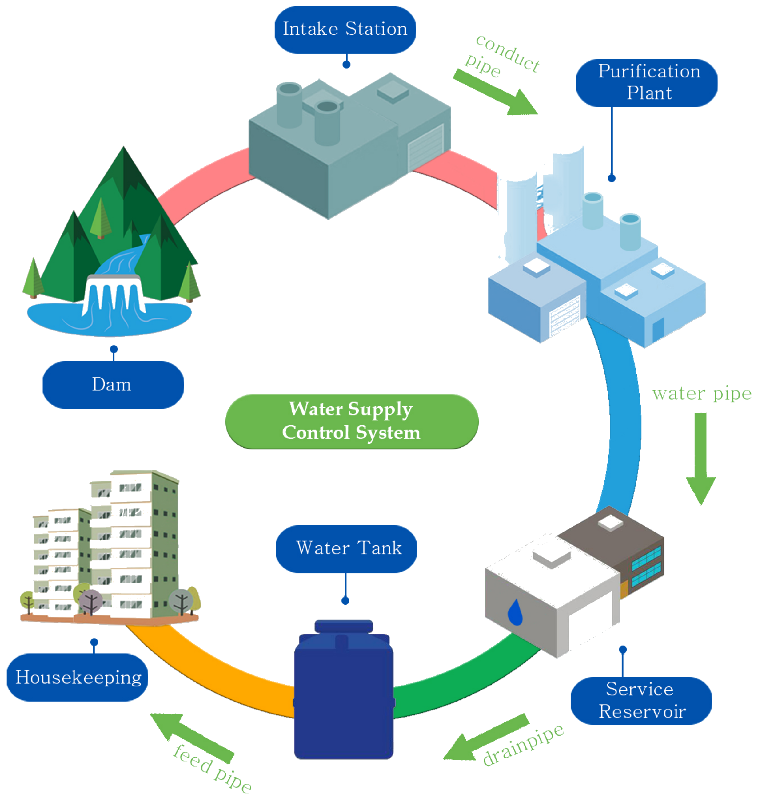
Figure 1. Water supply and sewage system.
Water 16 02631 g001
Figure 2. LSTM-autoencoder architecture.
Water 16 02631 g002
Figure 3. Proposed framework.
Water 16 02631 g003
Figure 4. Actual valve installation site.
Water 16 02631 g004
Figure 5. Completed sensor installation.
Water 16 02631 g005
Figure 6. Sensor installation close to the ground.
Water 16 02631 g006
Figure 7. Use case of leak detection.
Water 16 02631 g007
Figure 8. Leak data without noise.
Water 16 02631 g008
Figure 9. FFT for leak data.
Water 16 02631 g009
Figure 10. Actual and predicted values for data without noise.
Water 16 02631 g010
Figure 11. Actual and predicted values for data with noise.
Water 16 02631 g011
Figure 12. Noise attenuation.
Water 16 02631 g012
Figure 13. Accuracy.
Water 16 02631 g013
Figure 14. Precision.
Water 16 02631 g014
Figure 15. Recall.
Figure 15. Recall.
Water 16 02631 g015
Figure 16. F1 scores.
Water 16 02631 g016
Figure 17. AUC scores.
Water 16 02631 g017
Table 1. LSTM-autoencoder model.
SectionDescription
Encoder ArchitectureInput size: Size of input dimension
Hidden size: Size of hidden state in LSTM layer
Layers: Single LSTM layer
Decoder ArchitectureHidden size: Size of hidden state (same as encoder’s hidden size)
Output size: Size of output dimension (same as encoder’s input size)
Layers: Single LSTM layer
Autoencoder ArchitectureModel structure composed of encoder and decoder combination
Loss FunctionMean squared error (MSE)
OptimizerAdam optimizer
Learning rate: Value of learning rate (lr)
Training MethodEpochs: Total number of training epochs (num_epochs)
Early stopping: Early stopping with patience of 3 days
Batch size: Batch size for train_loader and val_loader
Model EvaluationModel evaluation using test loader
Measure model performance by returning average loss
Table 2. System specifications.
Hardware EnvironmentSoftware Environment
CPU: Intel Xeon Silver 4216 CPU @ 2.10 GHz
GPU: 4 x NVIDIA RTX A5000
Memory: 256GB DDR4
Storage: 2TB SSDOS: Ubuntu 18.04.6 LTS
Framework: TensorFlow 2.11.0
Programming Language: Python 3.10.9
Table 3. Performance comparisons.
ModelExisting ModelsProposed Models
Accuracy Precision Recall F1 Score Accuracy Precision Recall F1 Score
RandomForest0.95580.9790.95930.9690.98140.98550.98220.9838
XGB0.9570.98060.95930.96990.98270.98770.98220.9849
LogisticRegression0.80250.79060.98720.8780.98010.98650.97890.9827
KNeighbors0.95580.98450.95370.96890.98070.98440.98220.9833
DecisionTree0.94340.96830.95260.96040.98270.98770.98220.9849
ExtraTrees0.9530.97290.96150.96720.9820.98550.98330.9844
GradientBoosting0.95180.9740.95880.96630.98140.98550.98220.9838
AdaBoost0.95540.98060.95710.96870.98010.98220.98330.9828
SVC0.95540.98110.95650.96870.9820.98770.98110.9844
MLP0.93980.95460.96210.95840.97820.98220.980.9811
LGBM0.95140.9750.95710.9660.98140.98550.98220.9838
CatBoost0.95420.97570.96040.9680.9820.98660.98220.9844
Disclaimer/Publisher’s Note: The statements, opinions and data contained in all publications are solely those of the individual author(s) and contributor(s) and not of MDPI and/or the editor(s). MDPI and/or the editor(s) disclaim responsibility for any injury to people or property resulting from any ideas, methods, instructions or products referred to in the content.