Interpretation of Soil Characteristics and Preferential Water Flow in Different Forest Covers of Karst Areas of China

Abstract

Soil hydrology seriously affects the prevention of desertification in karst areas. However, water infiltration in the different soil layers of secondary forests and artificial forests in karst areas remains uncertain. This lack of clarity is also the factor that constrains local vegetation restoration. Therefore, monitoring and simulating the priority transport of soil moisture will help us understand the shallow soil moisture transport patterns after artificial vegetation restoration in the local area, providing a reference for more scientific restoration of the ecological environment and enhancement of carbon storage in karst areas. The integration of soil physical property assessments, computed tomography (CT) scanning, dye tracing studies, and HYDRUS-2D modeling was utilized to evaluate and contrast the attributes of soil macropores and the phenomenon of preferential flow across various forestland categories. This approach allowed for a comprehensive analysis of how the soil structure and water movement are influenced by different forest ecosystems and infiltration head simulations (5 mm, 15 mm, 35 mm, and 55 mm) to elucidate the dynamics of water movement across diverse soil types within karst regions, to identify the causes of water leakage due to preferential flow in secondary forests, and to understand the mechanisms of water conservation and reduction in artificial forests adopting a multifaceted approach. This study demonstrated that (1) the soil hydrological capacity of a plantation forest was 20% higher than a natural forest, which may be promoted by the clay content and distribution. (2) Afforestation-enhanced soils in karst regions demonstrate a significant capacity to mitigate the loss of clay particles during episodes of preferential flow and then improve the soil erosion resistance by about 5 times, which can effectively control desertification in karst area. (3) The uniform distribution of macropores in plantation forest soil was conducive to prevent water leakage more effectively than the secondary forest but was incapable of hindering the occurrence of preferential flow. The secondary forest had a very developed preferential flow phenomenon, and soil clay deposition occurred with an increase in depth. (4) Moreover, the results for preferential flow showed that the matrix flow depth did not increase with the increase in water quantity. Short-term and high-intensity heavy rainfall events facilitated the occurrence of preferential flow. Infiltration along the horizontal and vertical directions occurred simultaneously. These results could facilitate a further understanding of the contribution of the plantation to soil amelioration and the prevention of desertification in karst areas, and provide some suggestions for the sustainable development of forestry in karst areas where plantation restoration is an important ingredient.

1. Introduction

Karst landforms experience obvious leakage and possess fragile ecological environments [1]. These regions are susceptible to the threat of desertification. The forest canopy, understory vegetation, and the accumulation of dry branches and fallen leaves all play critical roles in water retention, soil erosion prevention, runoff management, and flood mitigation [2,3]. Restoring vegetation is key to addressing the conversion of soil water into a form that is accessible to plants [4]. Moreover, the strategic restoration of forest plantations can effectively tackle the ecological challenges mentioned above [5]. This approach not only enhances the ecological resilience of the area but also contributes to the overall sustainability of the landscape.

The growth of forestland in karst areas is limited by hydrologic circulation [6] and soil hydrologic properties [7]. Preferential flow is a significant contributor to soil dynamics [8]. This phenomenon involves the swift transportation of water through specific pathways, which can lead to the erosion of soil particles. Consequently, this process diminishes the soil’s shear resistance and overall structural stability [9]. Understanding the impact of preferential flow is crucial for developing effective soil management strategies aimed at maintaining soil health and preventing erosion. Moreover, it has an important effect on the restoration of ecological environments in ecologically fragile areas [10]. The lateral connectivity of soil macropores can promote lateral preferential flow and reduce covered soil stability [11]. Therefore, studying the difference between the contributions of plantation and natural forests to local soil water movement is necessary.

Many studies on preferential flow [12] in different areas, including snowy [13], dry [14], and red soil areas [15], exist. Studies on karst areas have mainly focused on the development, topological structure description [16], and modeling of large-scale karst pipelines [17]. Nevertheless, the focus on the survival, rehabilitation, and long-term sustainability of indigenous vegetation has often been overlooked. It is essential to investigate the interplay between local soil conditions and hydrological processes, especially in the context of vegetation growth. This study is vital because understanding this relationship is fundamental to fostering the sustainable management of desertification and its mitigation in karst regions [18]. By examining how vegetation influences soil and water dynamics, we can develop more effective strategies for ecological restoration and conservation in these ecologically sensitive areas. Dye tracing is a method that is commonly used to study preferential flow [19]. We combined computed tomography (CT) scanning and HYDRUS 5.03 simulation to compensate for the lack of continuous observation and the inability to restore the macropore topology accurately [20]. HYDRUS 5.03 is a versatile computer simulation package designed to model the movement of water [21], heat, and solutes [22] through three-dimensional or two-dimensional, variably saturated porous media. HYDRUS 5.03 is capable of handling a range of surface infiltration scenarios [23]. It is particularly adept at simulating the processes of water and solute transport within the soil matrix [24]. This capability makes HYDRUS a valuable tool for analyzing and predicting the behavior of fluids and their interactions with soil under various environmental conditions.

In this study, our objectives are (1) to clarify the soil physical properties, erodibility, macropore structure and preferential flow characteristics of different forestland types in the study area, to compare the improvement effect of different forestland types on soil, and (2) to simulate the soil water dynamic process and analyze the water-holding characteristics of different forestland types. The results of this study will help verify the importance of artificial restoration, provide data support for follow-up studies on desertification control in karst areas, and provide a reference for improving the measures of artificial forest restoration and sustainable development of forestry in karst desertification areas.

2. Materials and Methods

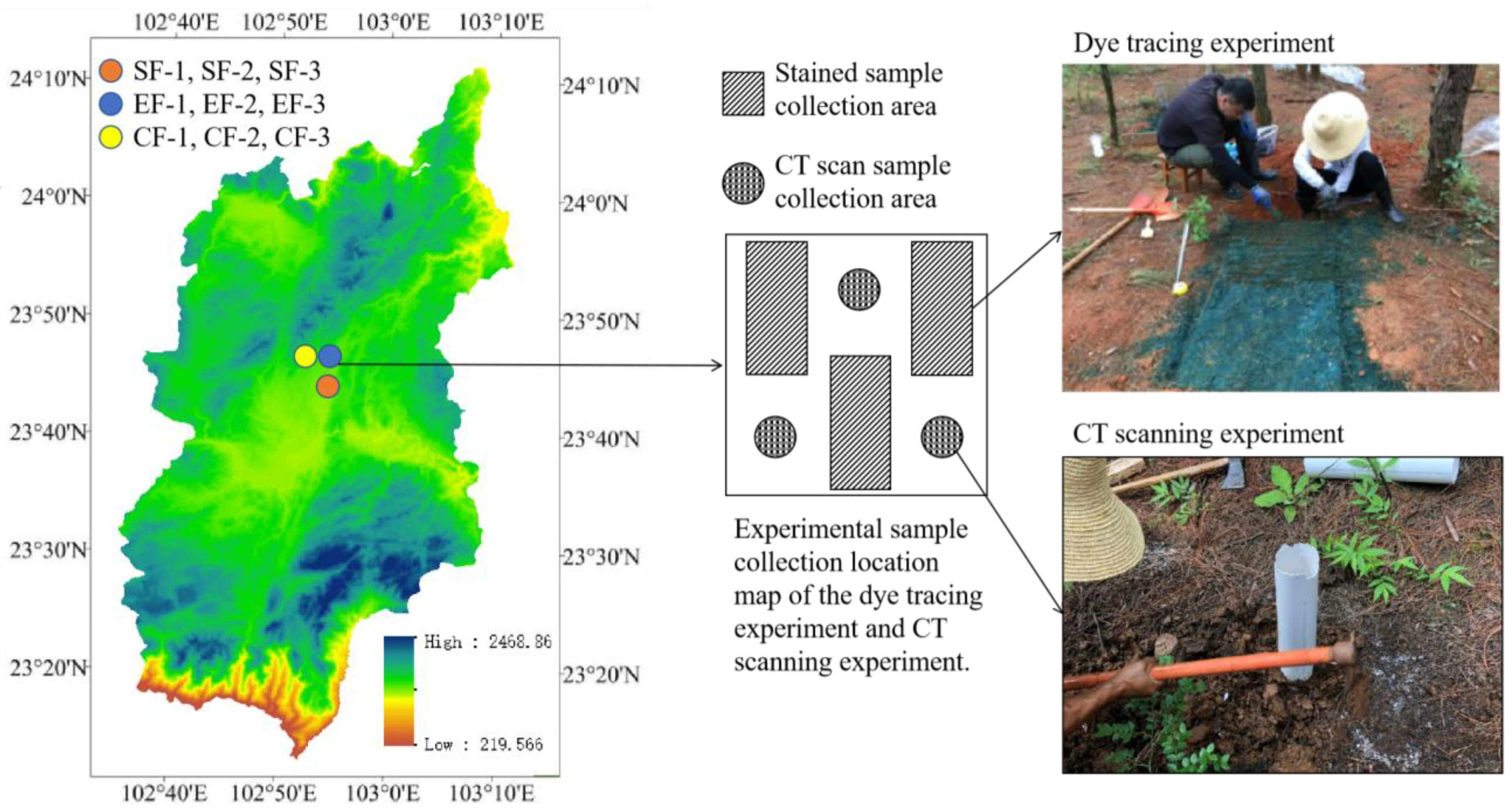
2.1. Environmental Characteristics of the Experimental Sites

Field studies were undertaken within a forested area located in the Yangjie Catchment, which is situated at coordinates 102°55′ East longitude and 23°37′ to 23°44′ North latitude (

Table 1. Overview of the experimental site characteristics.

Vegetation Type	Sample Number	Altitude (m.a.s.l.)	Latitude (N)	Longitude (E)	Slope (°)	Canopy Density (%)	Sand Content (%)	Silt Content (%)	Clay Content (%)
Secondary forest	SF1	1370	23°43′55″	102°54′54″	7	75	1.26 ± 0.61	20.34 ± 3.35	78.40 ± 3.63
	SF2	1370	23°43′53″	102°54′55″	7	80	0.52 ± 3.74	28.61 ± 5.62	70.87 ± 18.05
	SF3	1371	23°43′57″	102°54′52″	6	70	0.05 ± 4.82	21.20 ± 4.18	78.75 ± 7.57
	SF4	1371	23°43′57″	102°54′57″	9	80	1.15 ± 1.03	25.38 ± 3.39	75.54 ± 8.85
Eucalyptus robusta Smith plantation forestland	EF1	1370	23°37′21″	102°54′16″	4	82	2.82 ± 1.17	26.86 ± 2.27	70.32 ± 4.38
	EF2	1370	23°37′23″	102°54′13″	3	77	2.34 ± 1.58	42.93 ± 5.69	54.73 ± 1.06
	EF3	1370	23°37′20″	102°54′18″	3	80	3.41 ± 0.56	42.76 ± 8.08	53.83 ± 5.49
	EF4	1370	23°37′24″	102°54′25″	4	81	3.13 ± 2.73	38.94 ± 7.54	59.67 ± 0.78
Platycladus orientalis (L.) Francoptmxjjkmsc cypress plantation forestland	CF1	1370	23°37′13″	102°53′53″	2	60	9.86 ± 1.05	26.54 ± 5.77	63.6 ± 7.79
	CF2	1370	23°37′17″	102°53′48″	2	67	0.37 ± 1.84	14.48 ± 0.95	85.15 ± 4.41
	CF3	1370	23°37′20″	102°53′51″	2	65	0.77 ± 1.65	26.92 ± 0.50	72.31 ± 17.16
	CF4	1369	23°37′16″	102°53′56″	1	68	1.55 ± 2.91	23.21 ± 8.15	75.54 ± 1.06

, Figure 1). This region is part of the southwestern karst zone in Jianshui Town, Yunnan Province, China. The annual average temperature (air temperature measured in a louver box 1.5–2 m above the ground) is 19.8 °C and the annual average temperature of the land surface (the temperature measured on an unobstructed soil surface) is 20.8 °C. The average annual precipitation is 805 mm. The plantation forest was planted in 1985, and the secondary forest (SF) has been restored since 1970. Additional detailed information on the geology of the study area, the geomorphological characteristics of the environment, and a more extensive climatic description have been provided by Kan et al. [25]. Table 1 shows the basic information of the experimental sites.

2.2. Measurement of Soil Physical Properties

The soil depth under the conditions of the three vegetation types can all reach 50 cm or more; therefore, considering that the root systems of different types of vegetation have varying degrees of impact on the pore structure of soil at different depths during long-term growth, this study investigated each type of forest soil at 8 cm, 23 cm, and 40 cm soil depths, which represent soil within a depth range of 0–15 cm, 15–30 cm, and 30–50 cm. We employed the cutting ring immersion technique to ascertain the soil’s physical characteristics across various strata [26]. Once the surface litter was removed, soil samples for the cutting rings were obtained following a diagonal sampling pattern. Each cutting ring’s volume was standardized to approximately 100 cubic centimeters. The initial fresh mass of the soil was recorded as m₁. Subsequently, after allowing the cutting rings to absorb water for a duration of 12 h, they were swiftly weighed to obtain m₂. The moist soil samples were then spread out on a flat surface, with the cutting rings positioned mesh-end downward on a level platform, and their weights were recorded after 12 h of drainage as m₃. Following this, the samples were rehydrated, and after another 12 h, the weights of the rings were reassessed to obtain m₄. Finally, the cutting rings were exposed by removing their lids and then placed in a 105 degrees Celsius oven for a 24 h period to dry them thoroughly. This step ensured the accurate determination of the soil moisture content and other related physical properties. Then, we returned the upper cover and weighed the rings and filter paper immediately (m₅). The calculation formulas are as follows [27]:

$$P\left(\%\right)=\left[\left(m_1-m_4\right)/v\right]\times 100\%,$$

(1)

$$P_1\left(\%\right)=\left[\left(m_2-m_6\right)/v\right]\times 100\%,$$

(2)

$$P_2\left(\%\right)=P-P_1,$$

(3)

$$P_3\left(\%\right)=\left[\left(m_1-m_4\right)/\left(m_4-m_5\right)\right]\times 100\%,$$

(4)

$$P_4\left(\%\right)=\left[\left(m_2-m_4\right)/\left(m_4-m_5\right)\right]\times 100\%,$$

(5)

$$P_5\left(\%\right)=\left[\left(m_3-m_4\right)/\left(m_4-m_5\right)\right]\times 100\%,$$

(6)

$$P_6\left(\%\right)=\left[\left(m_1-m_4\right)/\left(m_4-m_5\right)\right]\times 100\%,$$

(7)

$$BD\left(\%\right)=\left[\left(m_4-m_5\right)/v\right]\times 100\%,$$

(8)

where P is the total porosity, P₁ is the capillary porosity, P₂ is the noncapillary porosity, P₃ is the maximum moisture capacity, P₄ is the minimum moisture capacity, P₅ is the field moisture capacity, P₆ is the natural moisture content of soil, and BD is the bulk density.

The saturated hydraulic conductivity was ascertained through the application of a steady water head in conjunction with a ST-70A soil moisture permeameter. Adhering to Darcy’s law, the formula for calculating the soil’s saturated hydraulic conductivity, denoted as K_s, is presented as follows [28]:

$$K_s={\displaystyle \frac{V}{tA}}·{\displaystyle \frac{L}{H}} ,$$

(9)

where K_s is the saturated hydraulic conductivity (cm·min⁻¹), H is the head pressure at the inlet end (cm), V is the amount of water passing through the cross-sectional area (cm³), t is the water outflow time (min), L is the length of the soil column (cm), and A is the cross-sectional area of the soil column (cm²).

The K value in the EPIC model [29] is used as an index to measure soil erodibility. The formula for K is as follows:

$$K=\left\{0.2+0.3exp\left[-0.0256SAN\left(1-{\displaystyle \frac{SIL}{100}}\right)\right]\right\}{\left({\displaystyle \frac{SIL}{CLA+SIL}}\right)}^{0.3}·\left(1.0{\displaystyle \frac{0.25C}{C+exp\left(3.72-2.95C\right)}}\right)\left(1.0{\displaystyle \frac{0.7SNI}{SNI+exp\left(-5.51+22.9SNI\right)}}\right) ,$$

(10)

where SAN is the sand content (%), SIL is the silt content (%), CLA is the clay content (%), C is the organic carbon content (%), and SNI = 1 − SAN/100.

2.3. Industrial CT Scan

The soil water path is closely related to soil structure [30,31]. A CT scanning experiment was performed to study the morphological characteristics of soil macropores in three forestland types. Nine undisturbed soil columns (PVC inner diameter of 10 cm, height of 30 cm, and pipe wall of 5 mm) were collected from a secondary forest (SF), eucalyptus plantation forest (EF), and cypress plantation forest (CF) because the metal pipe wall could affect the later scanning results. All of the columns were scanned using IPT4106D scanning equipment (Tsinghua Tongfang Co., Ltd., Beijing, China), a 4 MeV accelerator array CT scanning system. The undisturbed soil column was scanned in the form of a 2048 × 2048 CT image matrix with a resolution of 0.2 mm/pixels. Then, we used VG Studio MAX2.2 software to detect and calculate pore defects in the CT image stack automatically. Using a Gaussian filter, three-dimensional pore structural data could be obtained without destroying the whole soil structure. Part of the data was used to calculate characteristic macropore parameters [32], which mainly included the average diameter of macropores (d/mm), the total volume of pores (Vm/mm³), the total surface area of pores (Sm/mm²), and curvature (L_ti).

Under the assumption that each macropore was cylindrical, the ratio of volume (V) to the upper and lower surface area (S) could be used, that is, we used Formula (11) to calculate the actual length of the i-th layer macropores (L_ti):

$$L_{ti}={\displaystyle \frac{V}{S}}={\displaystyle \frac{V_i}{\pi {\left(\raisebox{1ex}{$d_i$}\!\left/ \!\raisebox{-1ex}{$2$}\right.\right)}^2}}$$

(11)

where V_i and d_i are the volume and diameter of the i-th layer macropores.

Curvature, denoted as L_ti, serves as an indicator of the degree of convolution in the macropore pathway, effectively capturing the extent of the flow object’s migration along the macropore channel. To quantify this characteristic, we applied Equation (12) to compute the cumulative curvature [32]. This approach allows for a detailed assessment of the macropore network’s structural complexity and its influence on the movement of water and other substances through the soil as follows:

$$L=\sum _{i=1}^n{\displaystyle \frac{L_{ti}}{L_{li}}}$$

(12)

where L_ti is the actual macropore length in the i-th layer (mm) and L_li is the vertical distance length in the i-th layer (mm).

2.4. Dyeing Experiment

We set up three groups of plots, each containing five vertical sections, in SF, EF, and CF to study the preferential flow development of different forest structures under different precipitation conditions. Before the test, residues and other covers on the surface of the sample site were removed to avoid interference. At each experimental site, PVC plates with a length × width × height of 0.6 m × 0.6 m × 0.3 m were used as enclosures and buried in the soil to a depth of 10 cm. Floating soil within 5 cm around the wooden frame was uniformly compacted with selenium. Ponding experiments were performed with 4 g/L bright blue dye to simulate 5 (light rain intensity, daily rainfall less than 10 mm), 15 (moderate rain intensity, daily rainfall between 10 mm to 25 mm), 35 (heavy rain intensity, daily rainfall between 25 mm to 50 mm) and 55 mm (heavy rain intensity, daily rainfall more than 50 mm) rainfall [33]. We designated these plots as G5, G15, G35, and G55 in accordance with the amount of the brilliant blue solution. The sample plot was covered with plastic film to prevent the interference of external factors on the dyeing test. After 24 h of dyeing, a 50 cm × 50 cm vertical section was excavated separately, and a Canon 500D digital camera (Canon (China) Co., Ltd., Beijing, China) with a resolution of 13 million pixels was used to take photos of the dyed section parallel to the sampled section. Adobe Photoshop CS6, IPWIN 6, and Origin 2019b were applied to convert dyeing images into numerical values for quantitative research. Kan et al. [25] provided detailed descriptions of the field sampling methods and image processing formulas for the calculation of the matrix flow depth (UF/cm), dye depth (ID/cm), dye area ratio (DC/%), priority flow ratio (PF), length index (Li/%), dye area ratio variation coefficient (CV), and dye depth variation coefficient (C μ).

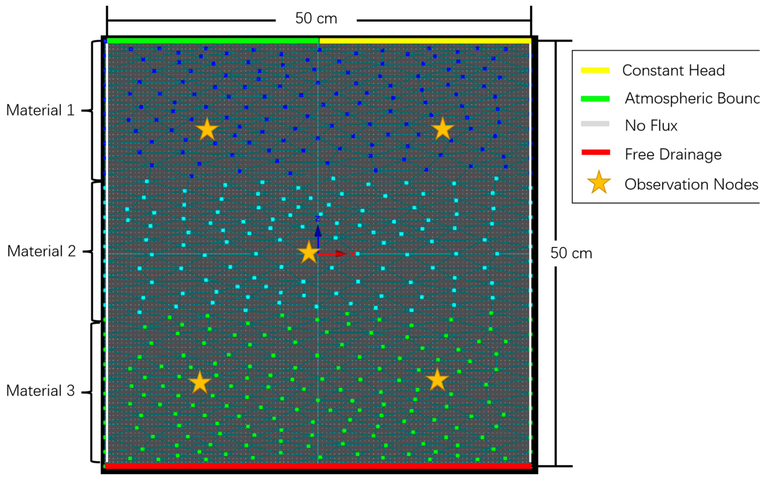
2.5. HYDRUS-2D Modelling

The HYDRUS-2D model is a powerful tool for simulating the movement of soil water and the transport of solutes [34,35]. The model employs the Richards equation to describe the flow control mechanism within the soil matrix. We selected the Galerkin finite-element equation under the assumption that the soil layers were uniform and isotropic and ignored the influence of air on soil flow movement [36,37] as follows:

$${\displaystyle \frac{\partial \theta }{\partial t}}={\displaystyle \frac{\partial }{\partial x}}\left[K(h){\displaystyle \frac{\partial h}{\partial x}}\right]+{\displaystyle \frac{\partial }{\partial z}}\left[K(h){\displaystyle \frac{\partial h}{\partial z}}\right]+{\displaystyle \frac{\partial K\left(h\right)}{\partial z}}$$

(13)

where θ is the soil volume moisture content (cm³ cm⁻³), h is the negative pressure water head (cm), K(h) is unsaturated hydraulic conductivity (cm min⁻¹), t is time (min), X is the horizontal coordinate (cm), Z is the upward positive vertical coordinate (cm), and the origin is at the upper boundary of the soil layer.

In order to compare the soil tax reporting capacity and water transport capacity under different vegetation restoration conditions, this study used the van Genuchten equations [38] to calculate the effective moisture content and unsaturated water conductivity as follows:

$${\theta }_e={\displaystyle \frac{\theta \left(h\right)-{\theta }_r}{{\theta }_s-{\theta }_r}}={(1+{\left|\alpha h\right|}^n)}^{-m}$$

(14)

$$K\left(\theta \right)=K_s{\theta }_e^{{\displaystyle \frac{1}{2}}}{\left[1-{\left(1-{\theta }_e^{{\displaystyle \frac{1}{m}}}\right)}^m\right]}^2$$

(15)

where θ_e is the effective water content; θ(h) is the soil volume water content (cm³ cm⁻³); θ_r is the residual water content (cm³ cm⁻³); h is the negative pressure water head (cm); α, n, and m are empirical parameters; K(θ) is the unsaturated water conductivity (cm min⁻¹); K_s is the saturated water conductivity (cm min⁻¹); and L is the pore curvature parameter, and CT scanning data were used to calculate L. We used Rosetta to estimate the hydraulic parameters (θ_r, θ_s, α, and n) required for the HYDRUS-2D model [39]. In this work, a square with a side length of 50 cm was used in the simulation of preferential flow motion, and the boundary conditions are shown in Figure 2.

2.6. Statistical Analysis

The data in this study were organized and processed using Microsoft Excel 2019, and the statistical analysis was performed using SPSS 24.0 software and Origin Pro 2021b software for plotting; Pearson’s correlation analysis was used to analyze the relationship between soil preferential flow and various environmental factors under different vegetation conditions and water infiltration rates.

3. Results

3.1. Physical Properties of Soil

Table 2. Soil physical conditions at different sites (means ± standard deviations).

Site Type	Depth (cm)	P (%)	P1 (%)	P2 (%)	P3 (%)	P4 (%)	P5 (%)	P6 (%)	BD (%)
SF	0–15	38.93% ± 2.61%	35.76% ± 2.96%	3.17% ± 0.35%	31.07% ± 3.37%	28.56% ± 3.54%	26.68% ± 2.94%	22.67% ± 1.52%	1.26 ± 0.05
	15–30	34.82% ± 3.78%	33.32% ± 3.88%	1.50% ± 0.10%	31.51% ± 4.84%	30.16% ± 4.87%	27.95% ± 3.83%	24.49% ± 0.54%	1.11 ± 0.05
	30–50	44.63% ± 0.03%	38.62% ± 2.92%	6.02% ± 2.89%	44.90% ± 0.29%	38.83% ± 2.66%	36.35% ± 2.81%	22.04% ± 0.15%	0.99 ± 0.01
EF	0–15	37.30% ± 1.94%	35.97% ± 1.40%	1.33% ± 0.54%	31.00% ± 2.71%	29.88% ± 2.22%	27.60% ± 1.75%	29.24% ± 2.77%	1.05 ± 0.03
	15–30	39.15% ± 0.01%	37.08% ± 0.08%	2.07% ± 0.07%	40.51% ± 0.01%	38.37% ± 0.06%	36.74% ± 0.03%	35.13% ± 0.06%	0.98 ± 0.09
	30–50	40.20% ± 0.01%	39.92% ± 0.01%	0.28% ± 0.01%	40.07% ± 0.00%	39.79% ± 0.01%	36.77% ± 0.01%	35.39% ± 0.02%	1.04 ± 0.09
CF	0–15	44.17% ± 0.01%	41.50% ± 0.02%	2.67% ± 0.01%	38.38% ± 0.00%	36.06% ± 0.01%	33.74% ± 0.01%	27.46% ± 0.02%	1.15 ± 0.00
	15–30	37.46% ± 1.72%	35.76% ± 0.79%	1.70% ± 0.93%	33.59% ± 0.38%	32.10% ± 1.13%	29.99% ± 1.46%	27.70% ± 0.69%	1.12 ± 0.06
	30–50	40.80% ± 0.01%	36.72% ± 0.00%	4.08% ± 0.01%	33.77% ± 0.00%	30.39% ± 0.00%	28.61% ± 0.01%	27.94% ± 0.01%	1.21 ± 0.00

SF corresponds to secondary forests, EF corresponds to Eucalyptus robusta Smith plantation forestland, CF corresponds to Platycladus orientalis (L.) Francoptmxjjkmsc cypress plantation forestland, P corresponds to the total soil porosity, P1 corresponds to the soil capillary porosity, P2 corresponds to the soil noncapillary porosity, P3 corresponds to the maximum water capacity, P4 corresponds to the minimum water capacity, P5 corresponds to the field capacity, P6 corresponds to the natural soil moisture content, and BD corresponds to the bulk density.

shows the soil physical and water properties at different depths of different forestland types. The total soil porosity, soil capillary porosity, maximum water capacity, and minimum water capacity of the Eucalyptus robusta Smith plantation forestland were 17%, 20%, 27%, 31%, and 34% higher than those of secondary forests, respectively. The natural soil moisture content and bulk density of CF were 20% and3% higher than those of the secondary forests, respectively.

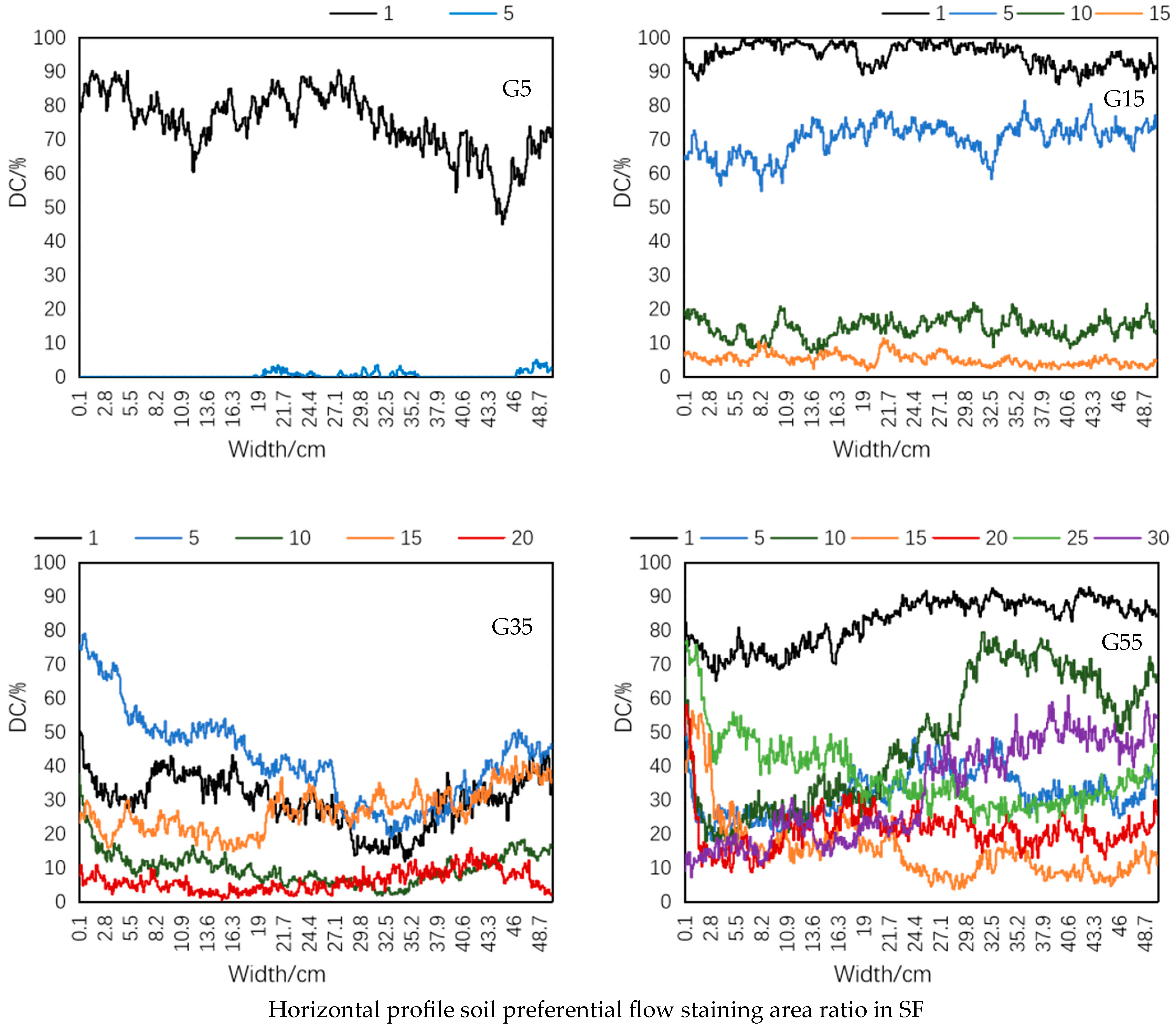
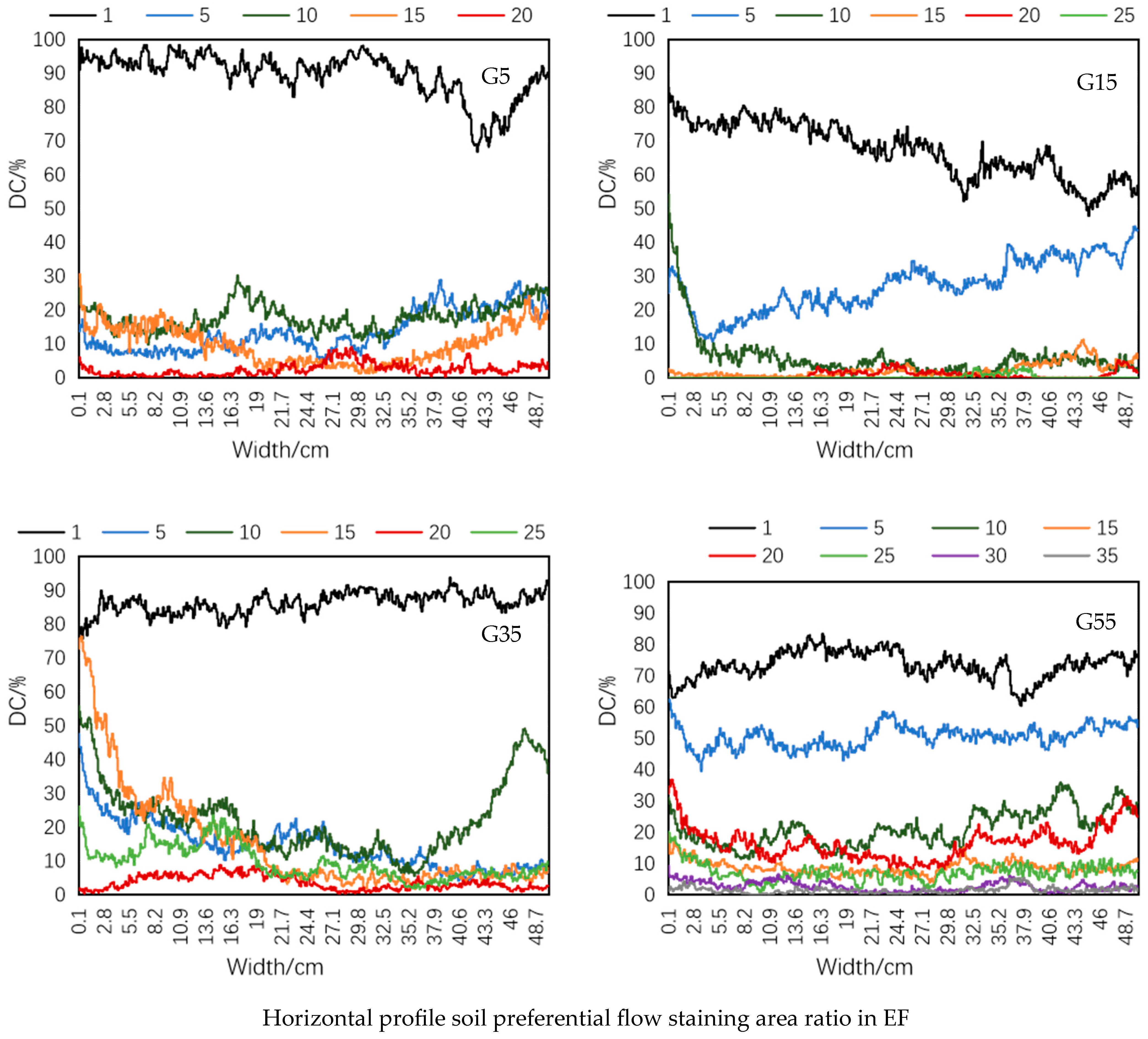
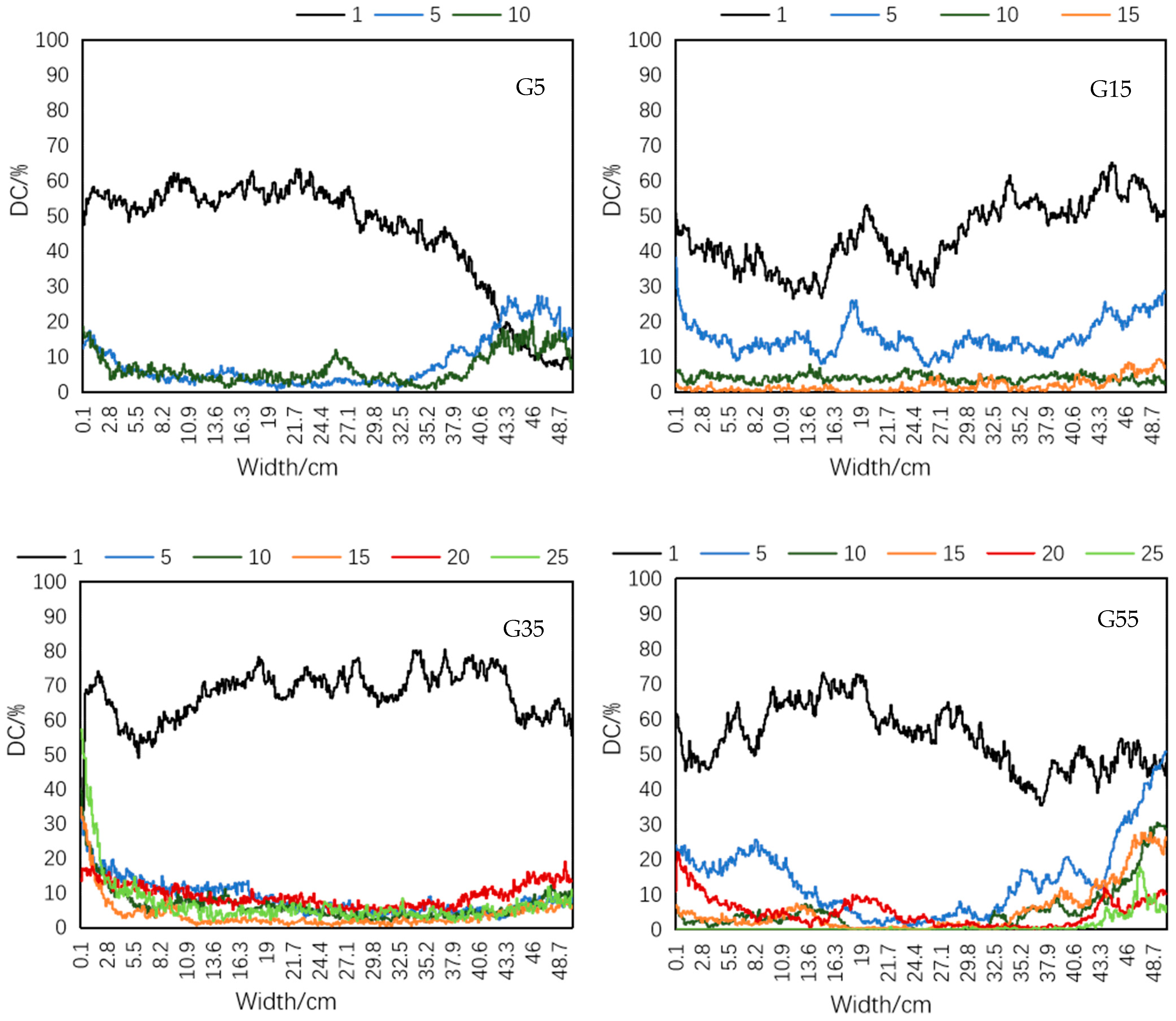
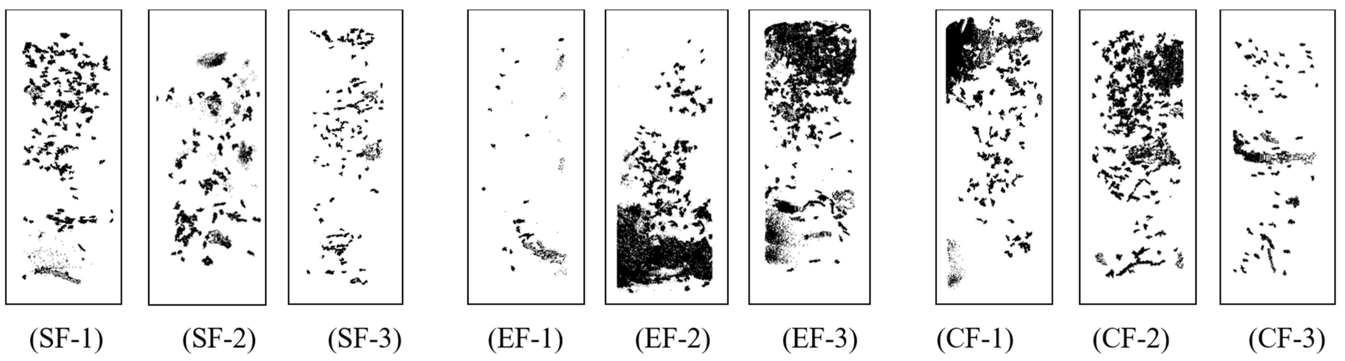
3.2. Dye Tracing Experiment

We conducted an analysis by examining 140 vertical stained soil sections from three distinct forest ecosystems following the early phase of an infiltration experiment, which spanned 24 h, and utilized the dye tracer brilliant blue FCF [40,41] (as depicted in Figure 3 and detailed in Table 2). Data where the dye concentration (DC) exceeded 80% were indicative of matrix flow and served as an indicator of the extent of the uniform infiltration front’s penetration [42]. This comparison allowed us to discern patterns and characteristics of water movement within the soil profiles of the different forest types.

Figure 3 lines (1), (5) illustrate that under the G5, G15, G35, G55 condition, all three types of forestland primarily exhibited matrix flow, with the occurrence of preferential flow being minimal or not readily apparent. This observation suggests a more uniform distribution of water infiltration across these forest soils under the specified condition. When the surface water exceeded 15 mm (G15), a significant preferential flow phenomenon existed and was most obvious in SF.

The preferential flow parameters of 140 soil profiles of the three kinds of forestland are provided in

Table 3. Preferential flow variables at the sample sites.

Site Type	Waterhead	Sample Number	UF/cm	ID/cm	DC/%	PF	Li/%	CV	Cμ
SF	G5	1	0.12 ± 0.04	5.10 ± 0.66	2.94 ± 1.30	0.99 ± 0.00	5.31 ± 2.16	0.41 ± 0.09	0.0020 ± 0.0012
		2	0.10 ± 0.06	7.26 ± 2.68	2.19 ± 0.62	0.99 ± 0.00
	G15	1	2.08 ± 1.13	22.78 ± 8.97	10.17 ± 1.98	0.96 ± 0.01	17.65 ± 4.51	0.42 ± 0.21	0.0028 ± 0.0002
		2	0.10 ± 0.06	11.72 ± 3.29	3.77 ± 2.12	0.99 ± 0.01
	G35	1	0.40 ± 0.60	17.34 ± 2.65	9.16 ± 3.52	0.99 ± 0.01	26.42 ± 0.59	0.37 ± 0.06	0.0012 ± 0.0001
		2	0.12 ± 0.04	16.7 ± 1.95	10.33 ± 2.92	1.00 ± 0.00
	G55	1	0.56 ± 0.74	25.94 ± 3.52	18.39 ± 3.41	0.99 ± 0.01	26.85 ± 1.46	0.21 ± 0.01	0.0010 ± 0.0001
		2	0.40 ± 0.28	25.40 ± 3.30	19.48 ± 3.86	1.00 ± 0.00
EF	G5	1	0.10 ± 0.00	14.70 ± 12.73	2.76 ± 2.10	0.98 ± 0.03	15.31 ± 4.64	0.48 ± 0.27	0.0037 ± 0.0023
		2	0.90 ± 1.41	8.36 ± 2.73	7.94 ± 2.54	0.98 ± 0.02
		3	0.40 ± 0.33	6.72 ± 1.05	5.29 ± 1.06	0.98 ± 0.01
	G15	1	1.48 ± 1.40	13.20 ± 2.98	7.76 ± 2.22	0.97 ± 0.03	17.94 ± 3.24	0.40 ± 0.17	0.0019 ± 0.0003
		2	0.46 ± 0.46	16.72 ± 2.69	7.60 ± 1.74	0.99 ± 0.01
		3	1.88 ± 1.81	14.12 ± 3.63	7.14 ± 4.05	0.96 ± 0.03
	G35	1	1.80 ± 1.20	7.24 ± 1.78	7.05 ± 0.97	0.95 ± 0.03	11.84 ± 6.01	0.27 ± 0.13	0.0026 ± 0.0008
		2	0.88 ± 0.39	10.20 ± 2.60	4.77 ± 0.82	0.96 ± 0.01
		3	0.88 ± 0.78	6.92 ± 3.45	5.48 ± 2.24	0.97 ± 0.02
	G55	1	0.44 ± 0.68	9.66 ± 3.25	6.67 ± 2.23	0.99 ± 0.01	21.14 ± 11.60	0.38 ± 0.15	0.0032 ± 0.0014
		2	0.10 ± 0.00	8.04 ± 1.35	4.15 ± 0.77	1.00 ± 0.00
		3	0.62 ± 0.85	13.34 ± 7.42	7.46 ± 3.78	0.99 ± 0.01
CF	G5	1	0.10 ± 0.00	8.36 ± 2.95	3.12 ± 1.81	0.98 ± 0.02	11.37 ± 4.92	0.66 ± 0.01	0.0034 ± 0.0006
		2	0.10 ± 0.00	4.68 ± 2.02	1.47 ± 0.88	0.97 ± 0.04
	G15	1	0.18 ± 0.16	15.40 ± 3.88	5.30 ± 2.12	0.99 ± 0.00	13.57 ± 3.87	0.41 ± 0.04	0.0029 ± 0.0006
		2	0.94 ± 0.72	7.98 ± 3.25	5.06 ± 1.68	0.97 ± 0.02
	G35	1	0.14 ± 0.08	5.10 ± 2.04	3.75 ± 0.73	0.99 ± 0.00	8.04 ± 0.13	0.18 ± 0.04	0.0033 ± 0.0002
		2	0.28 ± 0.22	6.78 ± 2.37	4.46 ± 0.57	0.99 ± 0.01
	G55	1	0.14 ± 0.08	3.86 ± 0.89	2.05 ± 0.77	0.98 ± 0.01	6.78 ± 1.79	0.39 ± 0.03	0.0032 ± 0.0012
		2	0.10 ± 0.00	7.28 ± 3.35	2.94 ± 0.93	0.99 ± 0.00

. The depth of matrix flow (UF/cm) is an indicator of the greatest extent to which water infiltrates uniformly. The infiltration depth (ID/cm) delineates the farthest reach of water infiltration in a non-uniform manner. Dye coverage (DC/%) serves to compare the variance in the stained areas at various depths, providing insights into the spatial distribution of the infiltration process. The preferential flow fraction (PF/%) indicates the extent and pattern of preferential flow within the soil profile. The length index of preferential flow (Li/%) is a metric that quantifies the level of heterogeneity present in the preferential flow pathways. The variation coefficient of dye coverage within the preferential flow areas (CV) offers a quantitative assessment of the variability in dye distribution after the exclusion of areas dominated by matrix flow. Similarly, the variation coefficient of maximum infiltration depths (Cμ) characterizes the variability and non-uniformity of soil water movement across vertical sections. In the context of the EF, the depth of matrix flow was observed to be 70% greater than that of SF, highlighting a significant difference in the infiltration capacity between these two types of forestland. The infiltration depth of SF was 1.8 times that of plantations, and the dye coverage of SF was 2 times more than that of plantations. The preferential flow fraction followed the order of SF > EF > CF. The length index of SF was 1.43 times that of the plantations, the variation coefficient of the dye coverage of CF was 1.16 times that of SF, and the variation coefficient of the dyeing depth of CF was 1.8 times that of SF.

3.3. CT Scanning Results

Nine soil columns were subjected to CT scanning and three-dimensional reconstruction (Figure 4). The vertically connected pores of SF were the largest. Vertical connectivity was strong, and connected pores were evenly distributed. However, pores with V_pore < 5 mm³ were few in number and highly concentrated in deep soil. Plantations had more medium pores (5 < V_pore < 10⁵ mm³) than SF. The vertical connectivity of CF was small, and the capillary porosity of CF was high and evenly distributed.

The total pore volume and surface area promoted the survival of water and the transportation of materials between soil and water (

Table 4. Results of industrial CT scanning.

Samples		SF			EF			CF
		1	2	3	1	2	3	1	2	3
d (mm)		1.26	1.18	1.24	1.15	1.23	1.25	1.27	1.19	1.20
Vm (104 mm3)		20.97	25.16	33.26	51.65	40.05	18.46	15.41	16.42	24.17
Sm (105 mm3)		11.65	17.76	20.43	37.55	20.38	10.99	9.03	14.06	18.34
L		0.55	0.53	0.86	0.56	0.47	0.51	0.48	0.62	0.55
Volume ratio (%)	<5 mm3	3.90%	4.79%	2.86%	2.71%	2.67%	6.53%	2.50%	14.61%	8.37%
	5–105 mm3	1.20%	0.58%	0.62%	0.14%	8.50%	8.05%	4.63%	4.78%	1.29%
	>105 mm3	94.89%	94.64%	96.52%	97.15%	88.83%	85.42%	92.87%	80.62%	90.35%

d is the average diameter, Vm is the total pore volume, Sm is the total pore surface area, and L is the curvature.

). The total pore volume and total surface area followed the order of EF > SF > CF. The total pore volume and total surface area of EF were 38% higher than those of secondary forests. The average diameter and curvature followed the order of SF > CF > EF, and the V < 5 mm³ of CF was twice that of secondary forests and Eucalyptus robusta Smith plantation forestland. The 5 < V < 10⁵ mm³ of EF was 6 times that of secondary forests (EF > CF > SF). V > 10⁵ mm³ followed the order of SF > EF > CF. Therefore, V < 5 mm³ was the highest in CF, 5 < V < 10⁵ mm³ porosity was highest in Eucalyptus robusta Smith plantation forestland, and V > 10⁵ mm³ porosity was highest in secondary forests.

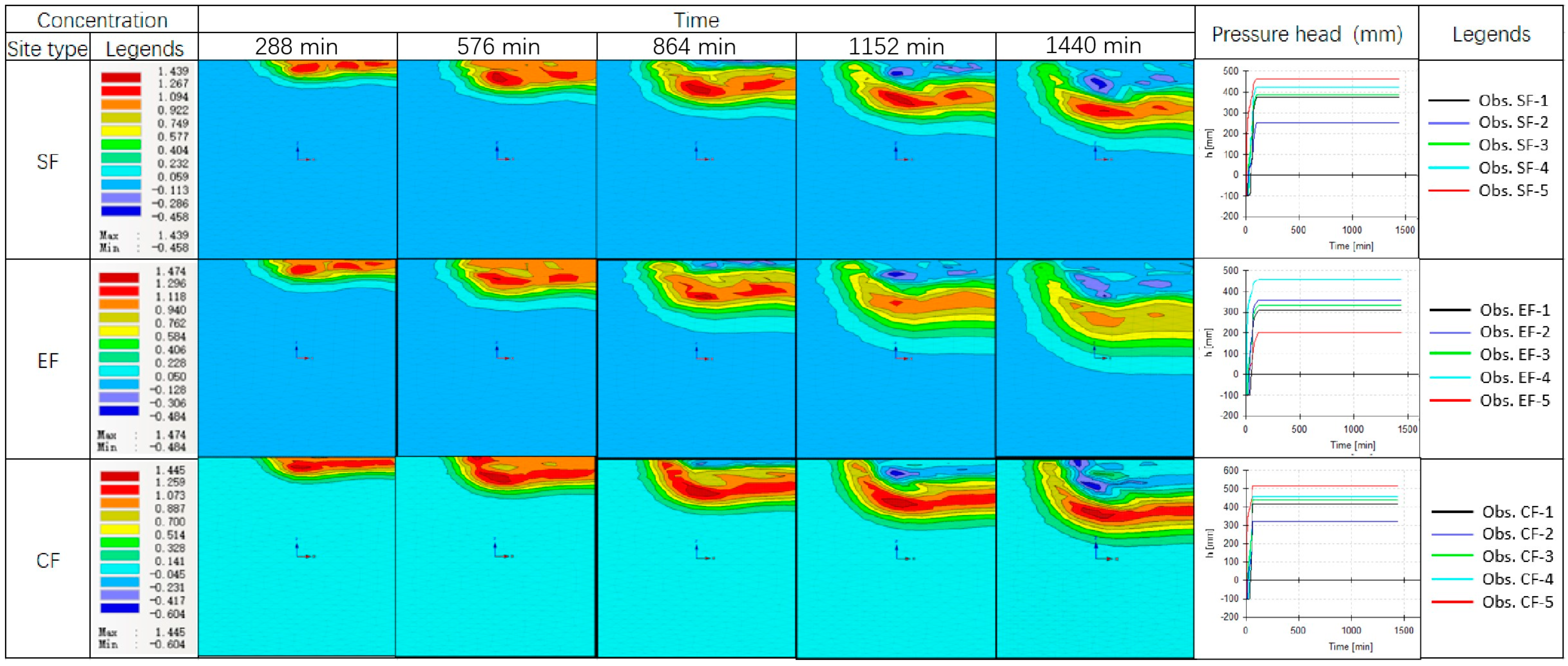
3.4. HYDRUS-2D Simulation of Different Flow Motions

Soil water flow movement in three forest land types (9 kinds of soil parameters) was simulated (

Table 5. Soil hydraulic parameters for the parameters of van Genuchten–Mualem model in HYDRUS [38].

Plot	Depth	Qr (cm3 cm−3)	Qs (cm3 cm−3)	Alpha (mm−1)	n (-)	Ks-S (cm day−1)	K (10−10)	Particle Size			Ks (cm·min−1)
								SAN (%)	SIL (%)	CLA (%)
SF	0–15	0.1068	0.5233	0.0198	1.1822	17.36	19.58	1.26	20.34	78.40	17.57
	15–30	0.1075	0.5269	0.0192	1.2117	19.04	14.37	0.52	28.61	70.87	13.54
	30–50	0.1077	0.5257	0.0199	1.1838	16.95	9.81	0.05	21.20	78.75	29.38
EF	0–15	0.1060	0.5223	0.0192	1.2082	19.03	29.11	2.82	26.86	70.32	48.67
	15–30	0.1063	0.5183	0.0155	1.3008	20.37	31.02	2.34	42.93	54.73	22.61
	30–50	0.1055	0.5156	0.0152	1.3050	20.05	38.90	3.41	42.76	53.83	35.14
CF	0–15	0.1019	0.5075	0.0189	1.2206	21.93	2.20	9.86	26.54	63.60	5.62
	15–30	0.1072	0.5206	0.0196	1.1657	17.67	4.09	0.37	14.48	85.15	6.05
	30–50	0.1073	0.5262	0.0194	1.2051	17.91	1.69	0.77	26.92	72.31	8.35

Notes: Qr is the residual water content, Qs is the saturated water content, Alpha and n are van Genuchten’s shape parameters, Ks-S is the simulated saturated hydraulic conductivity, L is the pore connectivity parameter, K is the soil erodibility factor (EPIC), SAN is the sand content, SIL is the silt content, CLA is the clay content, and Ks is the saturated hydraulic conductivity.

). Saturated hydraulic conductivity (Ks) represents the total amount of pores in the soil that could be used for water transport [43,44]. The soil erodibility factor (K) can indicate the sensitivity of soil to erosion. The soil erodibility factor followed the order of EF > SF > CF. We used G55 to simulate the preferential flow of soil (Figure 5). The simulated water content of each soil layer after surface water infiltration under nine kinds of soil moisture conditions is presented in Figure 6. Table 5 provides soil layer and depth data. Figure 6 presents the simulated water content of each soil layer. This value represents the simulated change in water contents under nine soil moisture conditions in three forestland types after surface water infiltration.

3.5. Statistical Analysis

A correlation analysis was conducted on all indicators in this study (

Table 6. Pearson’s correlation coefficients for this study.

	V	δ	τ	S	ξ	Ss	P	P1	P2	RF	TCR	P3	P4	P5	Ks	P6	Sa	Si	SCv	UF	ID	DC	PF	Li	CV	Cμ
V	1	0.281 *	−0.508 **	0.950 **	−0.590 **	0.545 **	0.423 **	0.369 **	0.261 *	−0.106	0.125	0.455 **	0.449 **	0.466 **	0.379 **	−0.203	−0.206	−0.013	0.151	0.041	0.164	0.147	0.065	0.081	−0.066	−0.095
δ		1	−0.279 *	0.336 **	−0.0629 **	0.292 *	0.107	−0.035	0.430 **	0.145	0.298 *	0.170	0.092	0.086	0.027	−0.126	−0.198	−0.150	0.256	−0.116	0.274 *	0.217	0.385 **	0.132	−0.212	−0.052
τ			1	−0.397 **	0.461 **	−0.072	−0.366 **	−0.317 *	−0.326 *	−0.026	−0.771 **	−0.313 *	−0.300 *	−0.330 *	0.027	0.293 *	0.315 *	0.254	−0.0421 **	0.407 **	0.091	0.254	−0.386 **	0.231	−0.157	0.106
S				1	−0.590 **	0.484 **	0.353 **	0.296 *	0.247	−0.194	0.078	0.421 **	0.414 **	0.424 **	0.414 **	−0.144	−0.237	−0.005	0.166	0.053	0.179	0.164	0.076	0.076	−0.136	−0.146
ξ					1	−0.184	−0.280 *	−0.197	−0.322 *	−0.240	−0.0433 **	−0.403 **	−0.374 **	−0.385 **	−0.296 *	0.012	0.375 **	−0.033	−0.230	0.078	−0.170	−0.145	−0.265 *	−0.059	0.249	0.161
Ss						1	−0.047	−0.065	−0.027	−0.150	−0.097	0.005	−0.014	−0.009	0.235	−0.167	0.105	0.121	−0.170	0.306 *	0.461 **	0.362 **	−0.188	0.312 *	0.019	0.175
P							1	0.948 **	0.477 **	0.107	0.153	0.856 **	0.863 **	0.858 **	0.090	0.339 **	−0.037	−0.195	0.183	−0.295 *	−0.158	−0.127	.281 *	−0.071	0.012	−0.077
P1								1	0.189	0.084	0.154	0.752 **	0.808 **	0.800 **	0.148	0.392 **	−0.061	−0.163	0.173	−0.285 *	−0.184	−0.172	0.229	−0.097	0.077	−0.064
P2									1	0.131	0.145	0.562 **	0.430 **	0.438 **	−0.138	−0.042	0.051	−0.190	0.118	−0.206	0.011	0.048	0.330 *	0.000	−0.114	−0.065
RF										1	0.037	0.155	0.142	0.138	−0.055	0.102	−0.085	−0.032	0.084	0.157	0.348 **	0.410 **	0.283 *	0.325 *	−0.132	0.183
TCR											1	0.191	0.200	0.220	−0.144	0.055	−0.444 **	−0.189	0.457 **	−0.503 **	−0.178	−0.373 **	0.436 **	−0.358 **	0.143	−0.158
P3												1	0.987 **	0.983 **	0.275 *	0.466 **	−0.172	−0.034	0.145	−0.206	0.030	0.058	0.331 *	0.032	−0.201	−0.141
P4													1	0.993 **	0.314 *	0.510 **	−0.194	−0.016	0.146	−0.211	0.006	0.030	0.307 *	0.013	−0.179	−0.149
P5														1	0.296 *	0.478 **	−0.207	−0.018	0.157	−0.228	−0.034	−0.016	0.312 *	−0.024	−0.163	−0.141
Ks															1	0.151	−0.123	0.395 **	−0.235	0.275 *	0.240	0.338 **	−0.041	0.283 *	−0.209	−0.097
P6																1	−0.128	−0.023	0.106	−0.087	−0.039	−0.009	0.130	−0.018	−0.112	−0.076
Sa																	1	−0.108	−0.597 **	0.206	−0.057	0.028	−0.434 **	0.111	0.042	0.168
Si																		1	−0.733 **	0.145	0.094	0.147	−0.095	0.094	−0.221	0.019
SCv																			1	−0.259 *	−0.037	−0.138	0.374 **	−0.152	0.149	−0.130
UF																				1	0.581 **	0.742 **	−0.669 **	0.711 **	−0.192	0.175
ID																					1	0.885 **	−0.051	0.778 **	−0.155	0.178
DC																						1	−0.173	0.853 **	−0.0374 **	0.125
PF																							1	−0.216	0.050	−0.102
Li																								1	−0.095	0.115
CV																									1	0.171
Cμ																										1

Notes: * p < 0.05, ** p < 0.01.

), and the results showed that the total stained area ratio of preferential flow was highly correlated with the saturated hydraulic conductivity, the preferential flow ratio was highly correlated with the macropore curvature, and the preferential flow length index was highly correlated with the matrix flow.

4. Discussion

4.1. Comparison of the Physical Properties of Soil

The types and activities of surface vegetation affect the physical properties of soil [45], and soil physical properties affect soil water infiltration and water loss [46], which both limit vegetation growth. The development of preferential flow in SF was better than that in plantations (Table 3), indicating that SF experienced long-term rapid water movement. This movement eroded soil particles [10], caused soil particle breakage (the soil erodibility factor in Table 5), and reduced shear resistance and soil stability. Meanwhile, preferential flow transported small soil particles to deep soil. These processes accounted for the largest clay content of SF (Table 5). A large amount of the clay content in SF was concentrated in deep soil (30–50 cm). Therefore, the diameter of soil particles in SF tended to decrease with an increase in depth. This relationship also indicated that SF experienced small-particle deposition. Shallow soil in SF (0–15 cm) had a low clay content and high organic matter content. In accordance with Formula (10), we found that although the shallow soil in SF was easy to erode, CF had the lowest the soil erodibility factor. Thus, the soil in CF had strong erosion resistance [47].

Moisture capacity is the amount of water in the soil that can be used for vegetation growth [48]. Table 2 shows that the maximum and field moisture capacities of EF were considerably higher than those of SF. Therefore, soil in EF had the highest amount of water available for vegetation, and its structure became highly conducive to water infiltration and storage after the accumulation of a large amount of water on its surface. The natural moisture content of CF was drastically higher than that of SF. Therefore, the soil structure of CF was conducive to the long-term storage of soil moisture needed for the growth of shallow ground vegetation when surface water infiltration decreased. Therefore, under the specific local soil structure conditions, the restoration of the plantation is conducive to local soil water storage and effectively reduces the formation of surface runoff.

Table 2 shows that the standard deviation of physical properties of the shallow soil (0–15 cm) in forestland was large and anisotropic. In contrast, the standard deviation of deep soil (30–50 cm) was generally small, likely because the soil structure was stable and obviously isotropic at deep depths. Soil was compact, and the soil structure was stable and similar. Pearson’s correlation coefficients were used to express the correlation between soil physical parameters. Similar to the conclusions of Jiang et al. [49], bulk density was negatively correlated with the field capacity and maximum capacity (Table 6).

4.2. Relationship between Macropores and Preferential Flow

The combined results of the preferential flow dye tracing experiment (Figure 3) and soil column scanning experiment (Figure 4) revealed differences in preferential flow and soil macropore characteristics under different vegetation community conditions [50]. The same soil layer showed different soil flow paths [47]. The dye coverage of SF increased inversely at 5–15 cm (Figure 3-SF). This behavior was significantly different from the behavior shown by the dye coverage of EF and CF. Moreover, the standard deviation of the dye coverage of SF was the largest, indicating that SF soil was prone to preferential flow under the condition of the local special soil structure. Figure 4 and Table 4 show that the number of macropores with V > 105 mm³ in SF was considerably higher than that in plantations. The vertical connectivity of the macropores is illustrated in Figure 4 CF had the highest number of macropores with V < 5 mm³ and lower characteristic parameters of preferential flow than SF (Table 3). In alignment with the research conducted by Jarvis et al. [47], our study also revealed that the presence, size, interconnectivity, and continuity of soil macropores are instrumental in facilitating preferential flow. Consequently, in the native forest soil, the vertical linkage of macropores was pronounced, with a scarcity of smaller pores. Such attributes augmented the ease with which surface water could infiltrate into the soil’s pore structure and elevated the soil’s permeability [51], indicating a heightened propensity for preferential flow development. This, in turn, could impede the soil’s capacity to retain water and potentially stunt the growth of surface vegetation [52]. On the contrary, in the soil of plantation forests, the pore structure was observed to be more stable, with pores across various diameter classes being uniformly distributed. These traits contributed to a more equitable redistribution of water, thereby fostering greater soil water retention and encouraging the growth of surface vegetation roots. The even distribution of pores supports a more balanced soil moisture profile, which is beneficial for both water conservation and plant development.

4.3. Influence of Different Vegetation Types on the Wetting Front of Preferential Flow

After studying the timeless physical properties of soil, we used HYDRUS-2D to combine preferential flow, soil physical properties, hydrological properties, and time. Table 5 shows that the trend followed by the simulated value of saturated hydraulic conductivity (Ks-S) was similar that shown by measured value (Ks). Both parameters exhibited a consistent trend that followed the order of EF > SF > CF. Our findings corroborate the conclusion reached by Niemeyer et al. [53], who determined that forest land generally has a higher saturated hydraulic conductivity compared to bare land. However, in the case of the EF, the measured saturated hydraulic conductivity exceeded the simulated values. This outcome is consistent with the results reported by Jiang et al. [49]. A high permeability rate facilitates the swift movement of excess surface water, which helps to prevent the development of surface runoff and enhances the soil’s ability to retain water [14]. Consequently, the early forest demonstrated a more robust water storage capacity compared to the secondary forest. This suggests that the soil in the early forest is more effective at managing water, reducing erosion risks, and supporting vegetation growth due to its superior water retention and infiltration characteristics.

Soil stratification impedes the downward progression of preferential flow pathways [51] while simultaneously promoting the lateral movement of water [54]. Figure 5 illustrates the lateral flow dynamics in soils with varying textures. However, the findings depicted in this figure diverge from those of Jiang et al. [49]. Jiang et al. concluded that lateral flow becomes pronounced in soil layers when a saturated zone emerges at the boundary between dissimilar soil materials, indicating a more complex interaction between soil stratification and water flow behavior. This discrepancy highlights the need for further investigation into how soil stratification affects the distribution and movement of water within different soil types. This difference may be due to the different time ranges of the two experiments. Lateral flow and wetting front formation occur simultaneously during the first 24 h of rapid infiltration. Compared to the 500 h long experimental results reported by Jiang et al. [49], this study compressed the most effective first 24 h experimental results, and the results were still similar. Therefore, the study of soil moisture infiltration can be analyzed based solely on the first 24 h of initial water infiltration. The wet front rapidly descended with the prolongation of time. The similar order of the water head size at each observation point in SF and CF (Figure 5) indicated that the water movement process and the hydraulic conductivity of soil were similar. Observation point 1 was mainly affected by lateral flow movement and followed the order of CF > SF > EF. Observation point 5 in SF and CF was the largest, indicating that vertical infiltration was dominant and obvious. However, observation point 4 in EF was the largest, indicating that lateral flow and vertical inflow in EF had great influences on hydraulic conductivity.

Figure 6 illustrates the moisture levels across various soil types. Initially, the moisture content of each stratum in the CF (controlled forest) was relatively uniform, as indicated in Table 2. Post-infiltration, however, the top layer from 0–15 cm depth exhibited the highest soil moisture content. Table 5 reveals that the sand content in the upper soil layer (0–15 cm) of CF was the highest, suggesting that a higher sand content aids in the soil’s rapid absorption of water over a brief period. This resulted in a significant amount of water being retained in the surface soil during the first 24 h of infiltration. Furthermore, CF’s maximum surface water retention capacity, denoted as P3 in Table 2, surpassed that of the secondary forest (SF) and the early forest (EF). In contrast, the water retention capacity of the middle soil layer (15–30 cm) in CF was the lowest among the compared types. This suggests a layered response to water infiltration, with the surface layer being particularly effective at holding water due to its composition, while the middle layer’s capacity was comparatively limited. Table 3 shows that the clay content of the middle layer (15–30 cm) of CF was large, and the high clay content stabilized the macropore structure [55]. Therefore, the soil moisture conduction rate of CF was rapid, and CF did not easily form surface runoff. The shallow soil structure of CF was conducive to the infiltration and storage of water. The shallow soil (0–15 cm) moisture content of EF was the smallest, whereas the deep soil moisture contents of SF and EF were the largest. As inferred from the initial moisture contents of SF and EF in Table 2 and the results of the particle size analysis in Table 5, the shallow soil layer (0–15 cm) of EF had the largest clay content and the deep soil layer of EF had the largest sand content. Therefore, the deep soil layer of EF has a strong water storage capacity and can store a large amount of water for a long time [56]. However, the initial water content of EF was higher than that of CF (Table 5) and the macropore connectivity was strong (Figure 4), which inhibited the lateral movement of water in macropore channels to the soil matrix and promoted preferential flow [57]. These results also accounted for the larger dyed area of EF (Figure 3) than that of CF. Therefore, simulation and field measurements showed that the saturated water holding capacity and capacity function of artificial forests were better than those of SF (Table 5 and Figure 5), and the soil structure of artificial forest was more conducive to improving the storage and regulation of local soil water than that of SF.

5. Conclusions

The water storage characteristics and dominant water movement characteristics of different soil types in secondary forests and plantations in a karst area were studied through experiments and simulation. About the soil physical properties, SF underwent soil particle deposition with the increase in depth, and the natural water content of CF was 20% higher than that of SF, and the available water of vegetation in the Eucalyptus robusta Smith plantation forestland was the highest (34% higher than that of secondary forests). Moreover, the soil erodibility factor of SF was 5 times higher than that of CF. About the macropore structure, the scanning results for the undisturbed soil column illustrated that macropores in secondary forests were vertically connected, and the distribution of the pore size and macropores in plantations was uniform. The results of the dye tracing experiment indicated that secondary forests in the karst area were prone to preferential flow, the depth of matrix flow did not increase with the increase in water quantity, and short-term and high-intensity heavy rainfall events facilitated preferential flow. The results of the simulation and field experiments indicated that the saturated water holding capacity and capacity function of plantations are better than those of secondary forests, and the soil structure of plantations is highly conducive to improving and repairing the storage and regulation of soil moisture in local karst areas. Therefore, studying soil preferential infiltration is crucial for vegetation restoration in desertified areas. In the future, further simulation of water transport after vegetation restoration in karst areas can be carried out, and based on the mechanism of water transport, can be combined with artificial intelligence methods to predict the underground water transport process, providing support for the sustainable development of different types of vegetation in the local area.

References

1. Hou, F.; Cheng, J.; Zhang, H.; Wang, X.; Shi, D.; Guan, N. Response of preferential flow to soil–root–rock fragment system in karst rocky desertification areas. Ecol. Indic. 2024, 165, 112234. [Google Scholar] [CrossRef]
2. Jordán, A.; Martínez-Zavala, L.; Bellinfante, N. Heterogeneity in soil hydrological response from different land cover types in southern Spain. Catena 2008, 74, 137–143. [Google Scholar] [CrossRef]
3. Yeshaneh, E.; Salinas, J.L.; Blöschl, G. Decadal trends of soil loss and runoff in the Koga catchment, northwestern Ethiopia. Land Degrad. Dev. 2015, 28, 1806–1819. [Google Scholar] [CrossRef]
4. Hu, L.; Zhou, Q.; Peng, D. Effects of vegetation restoration on the temporal variability of soil moisture in the humid karst region of southwest China. J. Hydrol. Reg. Stud. 2024, 53, 101852. [Google Scholar] [CrossRef]
5. Macias-Fauria, M. Satellite images show China going green. Nature 2018, 553, 411–413. [Google Scholar] [CrossRef] [PubMed]
6. Breshears, D.D.; Myers, O.B.; Barnes, F.J. Horizontal heterogeneity in the frequency of plant-available water with woodland intercanopy-canopy vegetation patch type rivals that occuring vertically by soil depth. Ecohydrology 2009, 2, 503–519. [Google Scholar] [CrossRef]
7. Iqbal, S.; Guber, A.K.; Khan, H.Z. Estimating nitrogen leaching losses after compost application in furrow irrigated soils of Pakistan using HYDRUS-2D software. Agric. Water Manag. 2016, 168, 85–95. [Google Scholar] [CrossRef]
8. Sohrt, J.; Ries, F.; Sauter, M.; Lange, J. Significance of preferential flow at the rock soil interface in a semi-arid karst environment. CATENA 2014, 123, 1–10. [Google Scholar] [CrossRef]
9. Dasgupta, S.; Mohanty, B.P.; Kohne, J.M. Impacts of juniper vegetation and karst geology on subsurface flow processes in the Edwards Plateau, Texas. Vadose Zone J. 2006, 5, 1076–1085. [Google Scholar] [CrossRef]
10. Verachtert, E.; Eeckhaut, M.V.D.; Poesen, J.; Deckers, J. Spatial interaction between collapsed pipes and landslides in hilly regions with loess-derived soils. Earth Surf. Process. Landf. 2013, 38, 826–835. [Google Scholar] [CrossRef]
11. McDonnell, J.J. A rationale for old water discharge through macropores in a steep, humid catchment. Water Resour. Res. 1990, 26, 2821–2832. [Google Scholar] [CrossRef]
12. Kogovsek, J.; Petric, M. Solute transport processes in a karst vadose zone characterized by long-term tracer tests (the cave system of Postojnska Jama, Slovenia). J. Hydrol. 2014, 519, 1205–1213. [Google Scholar] [CrossRef]
13. Avanzi, F.; Petrucci, G.; Matzl, M.; Schneebeli, M.; De Michele, C. Early formation of preferential flow in a homogeneous snowpack observed by micro-CT. Water Resour. Res. 2017, 53, 3713–3729. [Google Scholar] [CrossRef]
14. Guo, L.; Liu, Y.; Wu, G.-L.; Huang, Z.; Cui, Z.; Cheng, Z.; Zhang, R.-Q.; Tian, F.-P.; He, H. Preferential water flow: Influence of alfalfa (Medicago sativa L.) decayed root channels on soil water infiltration. J. Hydrol. 2019, 578, 124019. [Google Scholar] [CrossRef]
15. Yao, J.; Cheng, J.; Sun, L. Effect of Antecedent Soil Water on Preferential Flow in Four Soybean Plots in Southwestern China. Soil Sci. 2017, 182, 83–93. [Google Scholar] [CrossRef]
16. Rongier, G.; Collon-Drouaillet, P.; Filipponi, M. Simulation of 3D karst conduits with an object-distance based method integrating geological knowledge. Geomorphology 2014, 217, 152–164. [Google Scholar] [CrossRef]
17. Kaufmann, G. Modelling karst aquifer evolution in fractured, porous rocks. J. Hydrol. 2016, 543, 796–807. [Google Scholar] [CrossRef]
18. Flury, M.; Flühler, H. Tracer characteristics of brilliant blue FCF. Soil Sci. Soc. Am. J. 1995, 59, 22–27. [Google Scholar] [CrossRef]
19. Ghodrati, M.; Jury, W.A. A field study using dyes to characterize preferential flow of water. Soil Sci. Soc. Am. J. 1990, 54, 1558–1563. [Google Scholar] [CrossRef]
20. Katuwal, S.; Norgaard, T.; Moldrup, P.; Lamandé, M.; Wildenschild, D.; de Jonge, L.W. Linking air and water transport in intact soils to macropore characteristics inferred from X-ray computed tomography. Geoderma 2015, 237, 9–20. [Google Scholar] [CrossRef]
21. Navin, K.C.; Twarakavi, J.S.; Sophia, S. Evaluating Interactions between Groundwater and Vadose Zone Using the HYDRUS-Based Flow Package for MODFLOW. Vadose Zone J. 2008, 7, 757–768. [Google Scholar]
22. El-Nesr, M.N.; Alazba, A.A.; Šimůnek, J. HYDRUS simulations of the effects of dualdrip subsurface irrigation and a physical barrier on water movement and solute transport in soils. Irrig. Sci. 2014, 32, 111–125. [Google Scholar] [CrossRef]
23. Karandish, F.; Šimůnek, J. A comparison of the HYDRUS (2D/3D) and SALTMED models to investigate the influence of various water-saving irrigation strategies on the maize water footprint. Agric. Water Manag. 2019, 213, 809–820. [Google Scholar] [CrossRef]
24. Nohra, J.S.A.; Madramootoo, C.A.; Hendershot, W.H. Modeling Phosphorus Transport in Soil and Water. In Proceedings of the 2004 ASAE Annual Meeting, Ottawa, ON, Canada, 1–4 August 2004. [Google Scholar]
25. Kan, X.; Cheng, J.; Hu, X.; Zhu, F.; Li, M. Effects of Grass and Forests and the Infiltration Amount on Preferential Flow in Karst Regions of China. Water 2019, 11, 1634. [Google Scholar] [CrossRef]
26. Dexter, A.R. Advances in Characterization of Soil Structure. Soil Tillage Res. 1988, 11, 199–238. [Google Scholar] [CrossRef]
27. Dexter, A.R.; Richard, G.; Arrouays, D.; Czyż, E.A.; Jolivet, C.; Duval, O. Complexed organic matter controls soil physical properties. Geoderma 2008, 144, 620–627. [Google Scholar] [CrossRef]
28. Klute, A.; Dirksen, C. Methods of soil analysis: Part 1—Physical and mineralogical methods. In Hydraulic Conductivity and Diffusivity: Laboratory Methods; American Society of Agronomy: Madison, WI, USA, 1986; pp. 687–734. [Google Scholar]
29. Williams, J.R. EPIC-Erosion/Productivity Impact Calculator: 2. User Manual; USDA. Agricultural Research Service: Beltsville, MD, USA, 1990.
30. Bronick, C.J.; Lal, R. Soil structure and management: A review. Geoderma 2005, 124, 3–22. [Google Scholar] [CrossRef]
31. Kutílek, M. Soil hydraulic properties as related to soil structure. Soil Tillage Res. 2004, 79, 175–184. [Google Scholar] [CrossRef]
32. Meng, C.; Niu, J.; Li, X.; Luo, Z.; Du, X.; Du, J.; Lin, X.; Yu, X. Quantifying soil macropore networks in different forest communities using industrial computed tomography in a mountainous area of North China. J. Soil Sediments 2017, 17, 2357–2370. [Google Scholar] [CrossRef]
33. Kan, X.; Cheng, J.; Hou, F. Response of Preferential Soil Flow to Different Infiltration Rates and Vegetation Types in the Karst Region of Southwest China. Water 2020, 12, 1778. [Google Scholar] [CrossRef]
34. Šimůnek, J.; Šejna, M.; van Genuchten, M.T. The HYDRUS Software Package for Simulating Two and Three-Dimensional Movement of Water, Heat, and Multiple Solutes in Variably-Saturated Media. Technical Manual, Version 1.0. 2006. Available online: https://www.pc-progress.com/en/Default.aspx?hydrus (accessed on 15 August 2024).
35. Šimůnek, J.; van Genuchten, M.T.; Šejna, M. Recent developments and applications of the HYDRUS computer software packages. Vadose Zone J. 2016, 15, 7. [Google Scholar] [CrossRef]
36. Celia, M.A.; Bouloutas, E.T.; Zarba, R.L. A general mass-conservative numerical solution for the unsaturated flow equation. Water Resour. Res. 1990, 26, 1483–1496. [Google Scholar] [CrossRef]
37. Richards, L.A. Capillary conduction of liquids through porous mediums. Physics 1931, 1, 318–333. [Google Scholar] [CrossRef]
38. Van Genuchten, M.T. A closed-form equation for predicting the hydraulic conductivity of unsaturated soils. Soil Sci. Soc. Am. J. 1980, 44, 892–898. [Google Scholar] [CrossRef]
39. Schaap, M.G.; Leij, F.J.; van Genuchten, M.T. ROSETTA: A computer program for estimating soil hydraulic parameters with hierarchical pedotransfer functions. J. Hydrol. 2001, 251, 163–176. [Google Scholar] [CrossRef]
40. Flury, M.; Flühler, H. Brilliant Blue FCF as a dye tracer for solute transport studies—A toxicological overview. J. Environ. Qual. 1994, 23, 1108–1112. [Google Scholar] [CrossRef] [PubMed]
41. Van Ommen, H.C.; Dijksma, R.; Hendrickx, J.M.H. Experimental assessment of preferential flow paths in a field soil. J. Hydrol. 1989, 105, 253–262. [Google Scholar] [CrossRef]
42. Bargués, T.A.; Reese, H.; Almaw, A. The effect of trees on preferential flow and soil infiltrability in an agroforestry parkland in semiarid Burkina Faso. Water Resour. Res. 2014, 50, 3342–3354. [Google Scholar] [CrossRef] [PubMed]
43. Reynolds, W.D.; Drury, C.F.; Tan, C.S.; Fox, C.A.; Yang, X.M. Use of indicators and pore volume-function characteristics to quantify soil physical quality. Geoderma 2009, 152, 252–263. [Google Scholar] [CrossRef]
44. Pulido-Moncada, M.; Ball, B.C.; Gabriels, D.; Lobo, D.; Cornelis, W.M. Evaluation of soil physical quality index S for some tropical and temperate medium-textured soils. Soil Sci. Soc. Am. J. 2014, 79, 9–19. [Google Scholar] [CrossRef]
45. Edwards, W.M.; Van, D.P.R.R.; Ehlers, W. A Numerical Study of the Effects of Noncapillary-Sized Pores Upon Infiltration1. Soil Sci. Soc. Am. J. 1979, 43, 851. [Google Scholar] [CrossRef]
46. Karsanina, M.V.; Gerke, K.M.; Skvortsova, E.B.; Mallants, D. Universal spatial correlation functions for describing and reconstructing soil microstructure. PLoS ONE 2015, 10, e0126515. [Google Scholar] [CrossRef] [PubMed]
47. Jarvis, N.J. A review of non-equilibrium water flow and solute transport in soil macropores: Principles, controlling factors and consequences for water quality. Eur. J. Soil Sci. 2007, 58, 523–546. [Google Scholar] [CrossRef]
48. Givi, J.; Prasher, S.O.; Patel, R.M. Evaluation of pedotransfer functions in predicting the soil water contents at field capacity and wilting point. Agric. Water Manag. 2004, 70, 83–96. [Google Scholar] [CrossRef]
49. Jiang, X.J.; Chen, C.; Zhu, X.; Zakari, S.; Singh, A.K.; Zhang, W.; Zeng, H.; Yuan, Z.-Q.; He, C.; Yu, S.; et al. Use of dye infiltration experiments and HYDRUS-3D to interpret preferential flow in soil in a rubber-based agroforestry systems in Xishuangbanna, China. Catena 2019, 178, 120–131. [Google Scholar] [CrossRef]
50. Bottinelli, N.; Zhou, H.; Boivin, P.; Zhang, Z.B.; Jouquet, P.; Hartmann, C.; Peng, X. Macropores generated during shrinkage in two paddy soils using X-ray micro-computed tomography. Geoderma 2016, 265, 78–86. [Google Scholar] [CrossRef]
51. Zhang, Z.; Peng, X.; Zhou, H.; Lin, H.; Sun, H. Characterizing preferential flow in cracked paddy soils using computed tomography and breakthrough curve. Soil Tillage Res. 2015, 146, 53–65. [Google Scholar] [CrossRef]
52. Noriaki, W.; Hikaru, K.; Takashi, S.; Yagi, M. Local non-vuggy modeling and relations among porosity, permeability and preferential flow for vuggy carbonates. Eng. Geol. 2018, 248, 197–206. [Google Scholar]
53. Niemeyer, R.J.; Fremier, A.K.; Heinse, R.; Chávez, W.; DeClerck, F.A. Woody vegetation increases saturated hydraulic conductivity in dry tropical Nicaragua. Vadose Zone J. 2014, 13, vzj2013-01. [Google Scholar] [CrossRef]
54. Germann, P.F.; Zimmermann, M. Directions of preferential flow in a hillslope soil. Quasi-steady flow. Hydrol. Process. 2005, 19, 887–899. [Google Scholar] [CrossRef]
55. Koestel, J.K.; Moeys, J.; Jarvis, N.J. Meta-analysis of the effects of soil properties, site factors and experimental conditions on solute transport. Hydrol. Earth Syst. Sci. 2012, 16, 1647–1665. [Google Scholar] [CrossRef]
56. Rousseva, S.; Kercheva, M.; Shishkov, T.; Lair, G.J.; Nikolaidis, N.P.; Moraetis, D.; Krám, P.; Bernasconi, S.M.; Blum, W.E.H.; Menon, M.; et al. Soil water characteristics of European SoilTrEC critical zone observatories. Adv. Agron. 2017, 142, 29–72. [Google Scholar]
57. Buttle, J.M.; McDonald, D.J. Coupled vertical and lateral preferential flow on a forested slope. Water Resour. Res. 2002, 38, 1–16. [Google Scholar] [CrossRef]
Figure 1. In situ sample collection area map.
Water 16 02319 g001
Figure 2. HYDRUS-2D modelling. The observation points are 1, 2, 3, 4, and 5, respectively, from left to right and from top to bottom. The atmospheric bound and constant head, respectively, represent the soil surface without and with water infiltration, and are used to more vividly describe the changes in the soil moisture front.
Water 16 02319 g002
Figure 3. Example dye images for horizontal soil sections in the three types of sites with different precipitation amounts. G5, G15, G35, and G55 correspond to 5, 15, 35, and 55 mm ponded water infiltration simulation and simulate the changes in ponded water under light rain, medium rain, heavy rain, and stormy conditions, respectively. The bottom column shows the average dye coverage (DC) (yellow curve) and standard deviation (black part) of the three sites.
Water 16 02319 g003aWater 16 02319 g003bWater 16 02319 g003c
Figure 4. Results of industrial CT scanning.
Water 16 02319 g004
Figure 5. Results of water migration during the initial 24 h of the experiment under G55 as simulated by HYDRUS.
Water 16 02319 g005
Figure 6. Soil water retention curves computed by HYDRUS-2D; 1 is 0–15 cm, 2 is 15–30 cm, and 3 is 30–50 cm.
Water 16 02319 g006