Identification of the Runoff Evolutions and Driving Forces during the Dry Season in the Xijiang River Basin

Abstract

During the dry season, river flow gradually diminishes, and surface water flow dries up. Therefore, the investigation of runoff during the dry season is of great practical significance for rational water allocation and water resource management. Based on hydrological station data from the Xijiang River Basin (XRB) from 1961 to 2020, this study examines the trend and periodic characteristics of dry-season runoff, identifies fluctuation and variability in dry-season runoff, and investigates the main circulation factor combinations influencing dynamic changes in dry-season runoff. The results indicate the following: (1) the characteristics of dry-season runoff variations are basically consistent across sub-basins in the XRB during the study period, with the minimum (21.96 × 10⁸ m³) and maximum (54.67 × 10⁸ m³) average monthly runoff occurring in February and October, respectively; (2) interannual-scale dry-season runoff exhibits periodicity of 3.53 years and 7.5 years; (3) using the Bayesian estimator of abrupt seasonal and trend change algorithm (BEAST), a seasonal abrupt point with a probability of 20.5% occurs in 1983, and the confidence interval for this abrupt point is from 1980 to 1986; (4) based on the cross wavelet approach, solar sunspots are identified as the primary circulation factor contributing to dry-season runoff in the XRB, exhibiting a significant 8–14 years resonance cycle of negative correlation with runoff during the high-energy phase from 1972 to 2006. These findings offer a new perspective on understanding the evolution of dry-season runoff and circulation factor variations, which are crucial for accurate prediction, early warning, and rational allocation of water resources during the dry season.

1. Introduction

Runoff is one of the most important surface water bodies on Earth, which plays a significant role in ecosystems [1,2,3]. Runoff during the flood season may lead to disasters such as floods and reservoir failures, damaging the health of ecosystems. During the dry season, runoff may lead to increased environmental pollution and decreased ecological diversity in rivers by affecting the natural flow and self-purification capacity of water bodies [4,5,6]. When the flow rate of rivers decreases, their pollution carrying capacity also decreases, making decrease in water quality one of the main challenges faced by ecosystems [7,8]. Furthermore, changes in runoff can also have impacts on biodiversity in ecosystems, potentially disrupting the natural hydrological rhythm of rivers and reducing habitat diversity [9]. Therefore, evaluating runoff changes is crucial for the rational regulation of water resources and protection of the ecological environment.

The runoff during the dry season primarily stems from precipitation and water storage replenishment within the basin, with the flow process generally exhibiting a stable recession pattern [10,11,12]. Base flow, as a crucial component of runoff, serves as the main supply source during the dry season. When the surface water flow decreases, the runoff occurs in the dry season, mainly relying on the groundwater sources in the Pearl River basin [13]. Additionally, the dry season predominantly transpires during periods of low or no rainfall, with the start and duration contingent upon river supply conditions. Thus, the “dry season” is the period with the lowest rainfall or the lowest water levels. The duration of the dry season within a year varies depending on the natural geographical and meteorological conditions of the basin [14,15,16]. For medium-sized reservoirs, runoff is primarily utilized for regional irrigation and power generation, particularly during the dry season when assessing its runoff evolution is essential for formulating corresponding water supply and power generation plans. Rivers exhibit low flow or even dry up during the dry season, thus research on the dry season is crucial for water scheduling and resource management [8,17,18,19].

Research on the evolution patterns of runoff during the dry season mainly focuses on analyzing the characteristics of water level and hydrological extremes, as well as exploring the causes of low water flow. From a water resource management perspective, understanding the significance of dry-season runoff patterns is becoming increasingly crucial, especially in arid climates because water availability is at its lowest when demand is at its peak [20]. In hydrological practice, the dry season represents a periodic cycle during which river flow undergoes changes. Additionally, dry season flow rates depend on a range of factors, including the extent and hydraulic characteristics of aquifers, river recharge and actual evapotranspiration, soil permeability, and topographical features [2,21,22]. Bing et al. [7] used wavelet theory to analyze the runoff characteristics during the dry season in the source regions of the Yangtze and Yellow Rivers, discovering that the complex Morlet wavelet can detect runoff periodicity at hydrological stations and that different river segments exhibit varying periodicity features. Risva et al. [1] constructed a framework for forecasting low flows during the dry season in Mediterranean rivers, which provided six-month forecasts of low flow and evaluated 25 Mediterranean rivers of varying sizes and flow dynamics. Duan et al. [4] examined the abrupt changes and annual variability trends in runoff and sediment inflow to and outflow from Hongze Lake from 1975 to 2015, finding that inflow runoff and sediment decreased after 2015. The hydraulic engineering and land use changes are the main reasons for the significant decrease and abrupt change of sediment inflow. Li et al. [2] found that dry-season runoff in the Yangtze River basin showed a significant increasing trend between 1956 and 2018, with thawed soil water and autumn rainfall being the primary sources of dry-season runoff.

The evolution of runoff is driven by multiple factors, and understanding these driving forces helps to clarify the underlying mechanisms of runoff processes, providing a scientific basis for improving runoff forecasts and guiding regional water resource management [20,23,24,25]. Current research on runoff driving forces primarily focuses on the impact of climate change and human activities [1,3,26,27]. Climate change manifests through changes in precipitation, temperature, evaporation, humidity, sunshine duration, and wind speed, all of which directly control runoff processes [28,29,30]. Among these factors, the timing of precipitation has a significant impact on the variability of runoff. Additionally, human activities such as land use changes, surface cover alterations, irrigation activities, and reservoir operations affect the hydrological cycle and runoff processes, altering regional water circulation, which in turn impacts runoff patterns [31,32]. Alongside these factors, atmospheric circulation patterns can increase the frequency and intensity of extreme climate events, influencing climate anomalies, with long-term and sustained atmospheric circulation anomalies impacting runoff processes [33,34]. Thus, the dry and wet patterns of runoff are influenced not only by the direct impact of climate change and human activities but also by the indirect effects of atmospheric circulation factors [35,36].

The impact of the installation and development of hydropower production on runoff is mainly reflected in runoff regulation [37]. By constructing hydropower stations, hydropower resources can be converted into electrical energy, while changing the spatiotemporal distribution of river runoff, thereby altering the spatiotemporal distribution of hydropower. The runoff regulation of hydropower stations is an engineering measure to improve the navigation conditions of rivers during the dry season by constructing reservoirs, redistributing river flow in different seasons, and improving the navigation conditions of rivers during the dry season [38]. The basic approach to runoff regulation is to use the capacity and discharge facilities of the reservoir to store and release water and make decisions on reservoir operation by balancing the water volume during the regulation period, thereby changing the spatiotemporal distribution of runoff [39].

In recent years, with the rapid advancement of urbanization and industrialization, the supply and demand dynamics for water have undergone significant changes in the Xijiang River Basin (XRB). The total water usage from the mainstream has notably increased, intensifying supply–demand conflicts and leading to more frequent and prolonged dry periods, with increasingly complex and variable water exchange relationships [40,41,42]. Particularly during drought years or consecutive drought years, the conflicts in water usage for urban living, industry, and agriculture become more acute, along with worsening riverine ecosystem issues. Water shortages have emerged as a bottleneck in the fast and sustainable economic development of the XRB [22,43]. For example, in 2011, river flows dropped rapidly due to inadequate replenishment, especially in the Pearl River Delta. Similarly, in early 2021, the XRB experienced an unusually severe dry period, with rainfall at only 70% of the multi-year average, leading to a steady decline in river flow, marking the driest period in over 60 years [13]. Additionally, from October 2021 to February 2022, persistent low upstream rainfall resulted in a severe drought, leaving reservoirs with significantly depleted water storage, with a nearly 80% reduction in adjustable water volume compared to multi-year averages [5].

Nevertheless, existing studies have mainly focused on the characteristics of changes in runoff throughout the entire time period but have paid less attention to the impact of circulation factors on dry-season runoff. Furthermore, previous studies have identified change point in runoff, but it may be difficult to quantify the uncertainty of these sudden changes. Still, the identification of trend and seasonal components around the change point can improve the understanding of the mechanism of runoff changes [44]. Given this context, this study aims to (1) identify the trends and periodicity in runoff patterns during dry seasons in the XRB from 1961 to 2020; (2) examine the variability in dry-season runoff during the study period; (3) explore the coupled effects of various circulation factors on dry-season runoff dynamics; and (4) discuss the impact of land use changes on runoff.

2. Study Area and Dataset

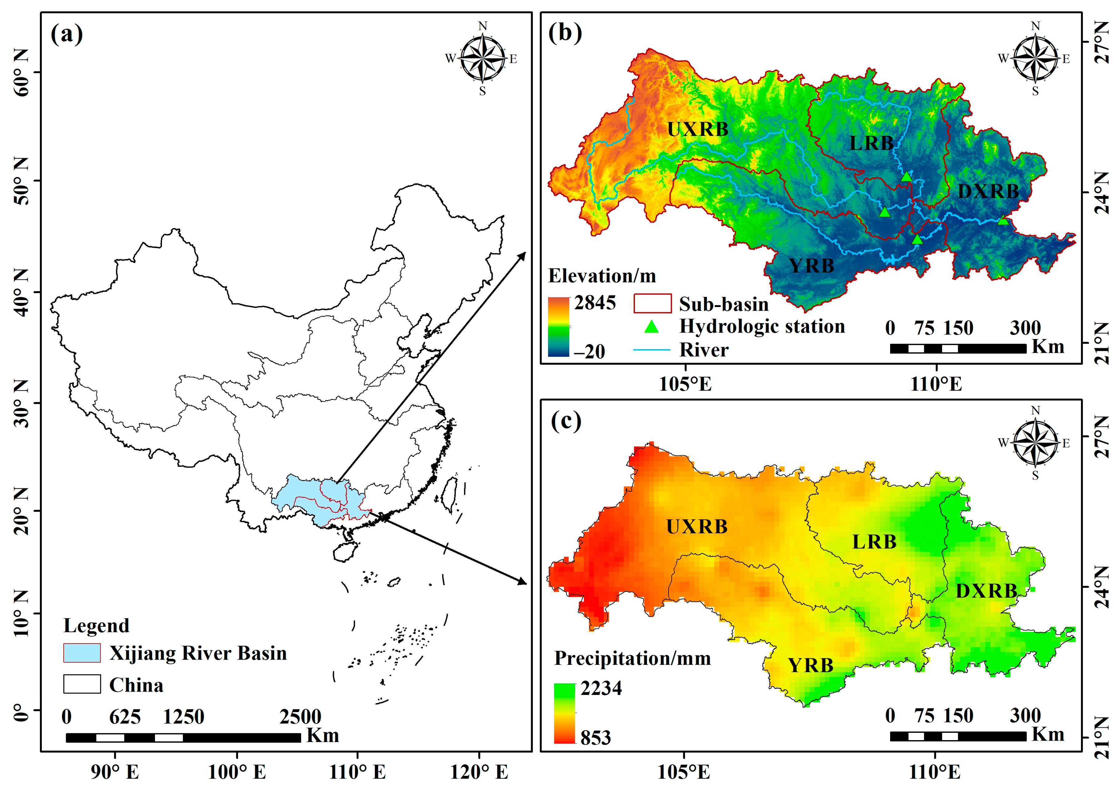
2.1. Study Area Description

The Pearl River Basin constitutes a complex river network system, where multiple rivers, including the Xijiang, Beijiang, and Dongjiang, converge with numerous tributaries in the Pearl River Delta region [41]. Among these, the Xijiang serves as the main stem, stretching 2214 km from its source in the Maxiong Mountains of Yunnan, traversing Guizhou and Guangxi, and finally discharging into the South China Sea via the Pearl River. With an annual average water resource of 230 billion m³, the XRB accounts for 68.5% of the total water resources in the entire Pearl River Basin. The natural flow of the Xijiang significantly influences the intrusion of saltwater into the Modaomen Waterway, and the salinity control through reservoir regulation in the upstream of the Xijiang helps alleviate water supply issues for the Greater Bay Area urban agglomeration. As depicted in Figure 1, the geographical scope of the XRB spans from 102°25′ E to 112°30′ E longitude and from 22°15′ N to 26°30′ N latitude, covering an area of 353,100 km², which represents 79% of the total area of the Pearl River Basin. The western part of the basin lies on the Yunnan-Guizhou Plateau, characterized by hills and basins, while the central region features a mixture of hills and basins, and the southeastern part comprises the delta plain formed by alluvial deposits, showing a gradual decrease in elevation from northwest to southeast with an average slope of 0.58%. The main sub-basins within the XRB include the upstream of Xijiang River Basin (UXRB), Liujiang River Basin (LRB), Yujiang River Basin (YRB), and the downstream of Xijiang River Basin (DXRB), with Wuzhou Station serving as the control station for the DXRB.

2.2. Dataset

This study utilizes monthly observed runoff data in four key hydrological stations from the Pearl River Water Resources Commission, i.e., Qianjiang, Liuzhou, Guigang, and Wuzhou, within the XRB from 1961 to 2020, representing the runoff variations in the UXRB, LRB, YRB, and DXRB, respectively. These hydrological stations are located at the outlet of the sub-basin, and can represent the runoff information of the sub-basin. One of the shortcomings of the hydrological data is the lack of data for certain months between 1988 and 2000. After preprocessing, some missing data are linearly interpolated using the adjacent station at the same time period with a strict quality control to ensure sequence continuity. The flow volume during each year’s dry season is defined as the total runoff from October of the current year to March of the following year. Investigating the impact of climatic factors on runoff facilitates the prediction of runoff trends and the rational development, allocation, and utilization of water resources, which is crucial for understanding the distribution of runoff in different regions and seasons [45,46]. Therefore, this study selects nine large-scale climate circulation factors from 1961 to 2020, including the El Niño—Southern Oscillation (ENSO), Pacific Decadal Oscillation (PDO), Arctic Oscillation (AO), Atlantic Multidecadal Oscillation (AMO), North Atlantic Oscillation (NAO), Dipole Mode Index (DMI), North Pacific Index (NPI), Pacific–North American (PNA), and Sunspot Index (SSI), and employs cross-wavelet analysis to explore potential driving forces behind runoff variations. The digital elevation model (DEM) data, acquired through photogrammetric methods, are widely used in hydrology, meteorology, landforms, geology, soil, and other scientific fields [47]. In this study, DEM data primarily originate from radar topographic survey data collected by the U.S. space shuttle Endeavour with a spatial resolution of 1 km. Land use is primarily based on Landsat remote sensing image data from the United States, which is manually interpreted visually with a spatial resolution of 1 km [48]. According to land resources and their utilization attributes, land use types are divided into crop land, forest land, grassland, water area, urban land, and unutilized land. The datasets used in this study are listed in

Table 1. The datasets used in this study.

Name	Date	Temporal Resolution	Spatial Resolution	Reference
Runoff	1961–2020	monthly	–	Tian et al. [41]
Large-scale climate circulation factors	1961–2020	monthly	–	Hadad et al. [45]
Digital elevation model	2020	–	1 km	Ahmad et al. [47]
Land use	1980–2020	yearly	30 m	Yang and Huang [48]

. Details on the station datasets are listed in

Table 2. Details on the station datasets.

Stations Names	Coordinates	Elevation (m)	Period	Temporal Resolution
Qianjiang	23°38′ N, 108°58′ E	77	1961–2020	monthly
Liuzhou	24°19′ N, 109°24′ E	101	1961–2020	monthly
Guigang	23°5′ N, 109°37′ E	48	1961–2020	monthly
Wuzhou	23°29′ N, 111°18′ E	16	1961–2020	monthly

.

3. Methodology

3.1. Extreme-Point Symmetric Mode Decomposition

To comprehend the nonlinear structures of complex system evolution accurately, Wang and Li developed a novel time–frequency analysis approach termed extreme-point symmetric mode decomposition (ESMD) [49]. Building upon the foundational principles of empirical mode decomposition (EMD), ESMD optimizes residual modes via the inclusion of the “least squares method”, thereby transforming them into an “adaptive global mean line” for precise determination of the optimal sifting times. This method enhances both adaptability and accuracy in data analysis while ensuring decomposition precision. As a time-varying signal adaptive analysis technique grounded in fractal principles, ESMD exhibits remarkable adaptability in analyzing time series data characterized by non-stationary and nonlinear features. It stands as one of the advanced methods utilized for extracting trends and periodic components from time series data. By smoothing complex time series, ESMD systematically separates multi-scale oscillatory components and their trend items within the original sequence. Through ESMD application, initial time series can be decomposed into several intrinsic mode functions (IMFs) along with a cumulative residual trend term (R), revealing the time-varying characteristics of each IMF in terms of amplitude and frequency and offering clear insights into the evolution process of total energy.

3.2. Bayesian Estimator of Abrupt Seasonal and Trend Change Algorithm

The changes in runoff during the dry season exhibit nonlinear and non-stationary characteristics. To overcome this problem, the Bayesian estimator of abrupt seasonal and trend change algorithm (BEAST) is adopted to decompose a time series based on Bayesian statistical theory, effectively avoiding issues such as uncertainty, overfitting, and model misspecification. BEAST quantifies the relative importance of a single model and uses a Bayesian model to average multiple models. As a Bayesian estimator algorithm for abrupt, seasonal, and trend detection, the BEAST provides probabilistic information regarding mutation points. Compared to deterministic estimation methods, its advantage lies in enhancing the accuracy of identifying abrupt points by presenting prior and posterior probability distributions, simultaneously using quantitative probability to describe the inevitable uncertainty in abrupt detection [23,50]. Based on the Bayesian framework, the BEAST decomposes the time series Y_τ into three parts:

$$Y_{\tau }=T_{\tau }+S_{\tau }+\epsilon ,$$

(1)

where T_τ represents the trend signal, S_τ represents the seasonal signal, and ε represents the residual signal. Assuming trend term T_τ detects τ₁, …, τ_m abrupt points, the linear expression for the trend term is

$$T_i={\alpha }_i+{\beta }_{i}t({\tau }_{i-1}<t<{\tau }_i,i=1,\dots ,m),$$

(2)

where i represents the site of abrupt point, and α_i and β_i represent the intercept and slope of the linear model on both sides of the abrupt point, respectively.

Seasonal term S_τ uses a periodic model via a flexible basis function (Fourier curve) for segmented fitting; the expression is

$$S_{\tau }={\displaystyle \sum _{k=1}^K{\gamma }_k\sin (\frac{2\pi k\tau }{f}+{\delta }_k)},$$

(3)

where γ_k, δ_k and f represent amplitude, phase, and frequency, respectively.

This study employs the Bayesian estimator algorithm to detect abrupt points in both the entire period and dry-season runoff sequences, thereby segmenting the entire runoff time series to reveal detailed characteristics of runoff variations in different stages. Additionally, the trend changes are categorized into eight types: monotonic increase (no abrupt point), monotonic decrease (no abrupt point), monotonic increase (positive abrupt point), monotonic decrease (negative abrupt point), interrupted increase, interrupted decrease, increase to decrease, and decrease to increase.

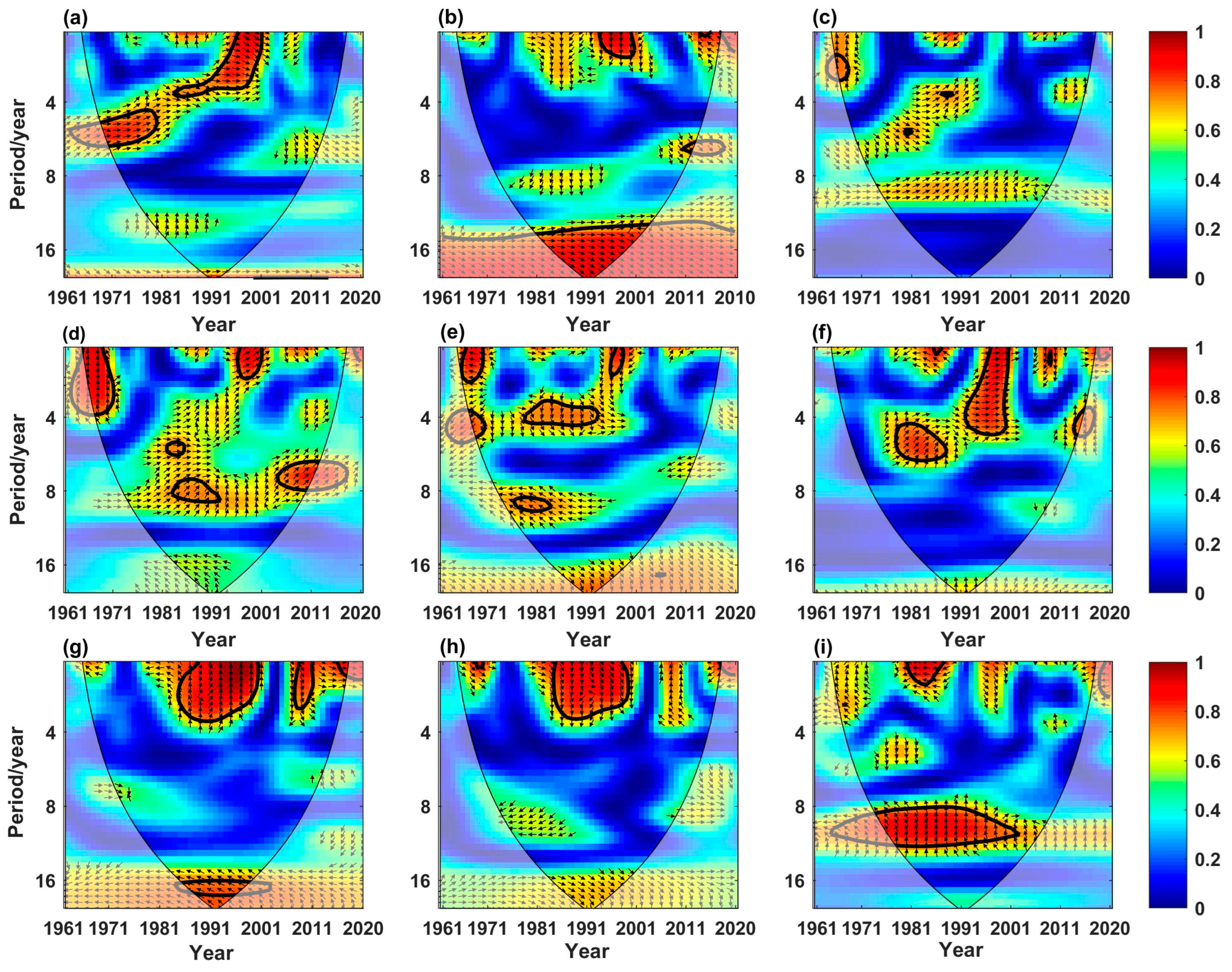
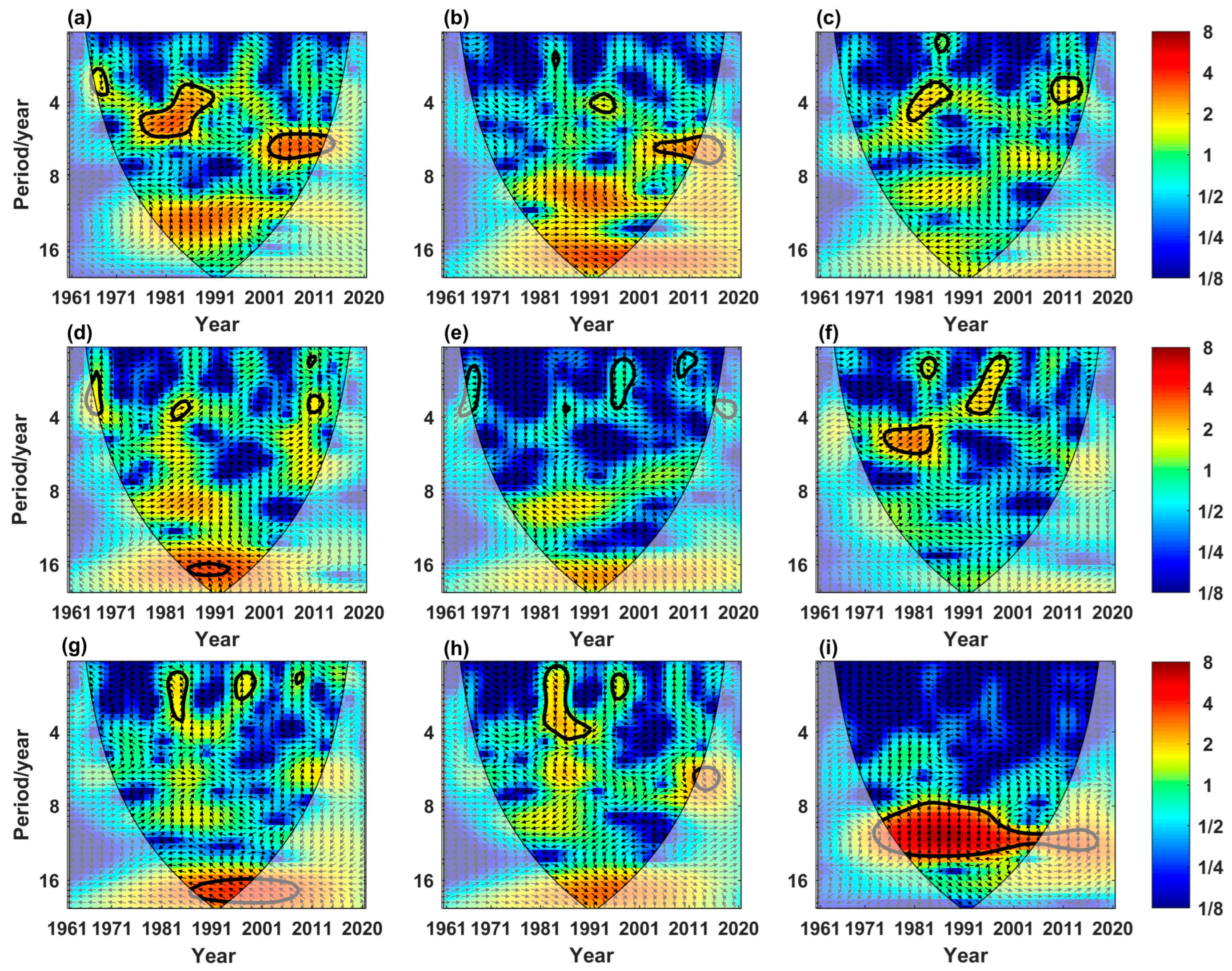
3.3. Cross Wavelet Transform Technology

In order to reveal the complex impact of circulation factors on dry-season runoff, we use a cross wavelet approach. The main advantage of cross wavelet is that it does not need to assume the distribution of data and can check the phase characteristics and correlation within non-stationary time series data from via time–frequency analysis [51]. Unlike Fourier analysis, it can address variations in spectral energy over time by emphasizing the importance of data in proximity to specific times [52]. As a method that transforms data from the time domain to the frequency domain, wavelet analysis identifies dominant modes of variability and their temporal evolution, enabling the detection of local periodicities (or frequency bands) associated with specific processes. Cross wavelet transform is a multiscale wavelet transform signal analysis technique that combines wavelet transform with cross-spectral analysis, used for multi-time–frequency analysis of dual time series. It can also determine the correlation by describing the phase relationship between two time series in time–frequency space, accurately diagnosing their time lag and phase structure. Given two time series X and Y with wavelet transform $W_n^X(s)$ and $W_n^Y(s)$, cross wavelet spectrum can be defined as

$$W_n^{XY}(s)=W_n^X(s)W_n^{Y\ast }(s),$$

(4)

where $W_n^{Y\ast }(s)$ represents the complex conjugation of $W_n^Y(s)$, s represents the time sequence, and n represents the length of s. The larger the value of $|W_n^{XY}(s)|$, the higher the cross-correlation coefficient.

The component of $W_n^{XY}(s)$ is employed to describe the phase between two time series, quantifying phase relationships by the circular mean of phases in regions with statistical significance >5%. Furthermore, the circular mean of a set of angles is defined as follows:

$$\overline{\alpha }=\arg (\overline{x},\overline{y}),\overline{x}={\sum }_{i=1}^n\cos ({\alpha }_i),\overline{y}={\sum }_{i=1}^n\sin ({\alpha }_i).$$

(5)

In wavelet diagrams, cross-wavelet phase angles are represented by arrows: ← denotes negative correlation between two sequences; → indicates in-phase variation, meaning they are positively correlated; ↓ signifies the preceding sequence shifts 90° forward; ↑ indicates the sequence lags 90° behind. Time delay is determined by the phase delay between two variables multiplied by their respective periods.

Although the technique of cross-wavelet analysis has the capability to detect relationships between two time series, it only reveals regions with high common power. In contrast, the wavelet coherence transformation can measure the overall coherence between two time series. Furthermore, the multiple wavelet coherence method is used to investigate the dependence relationship of a certain geophysical variable on the synergistic effects of multiple variables. This method is also based on the cross-wavelet power spectrum and auto-wavelet power spectrum between the variables. In wavelet analysis, the percentage of significant power (POSP) and the average wavelet coherence (AWC) are used to evaluate, quantitatively, the explanatory ability of the predictive variable for the response variable [51,52].

4. Results

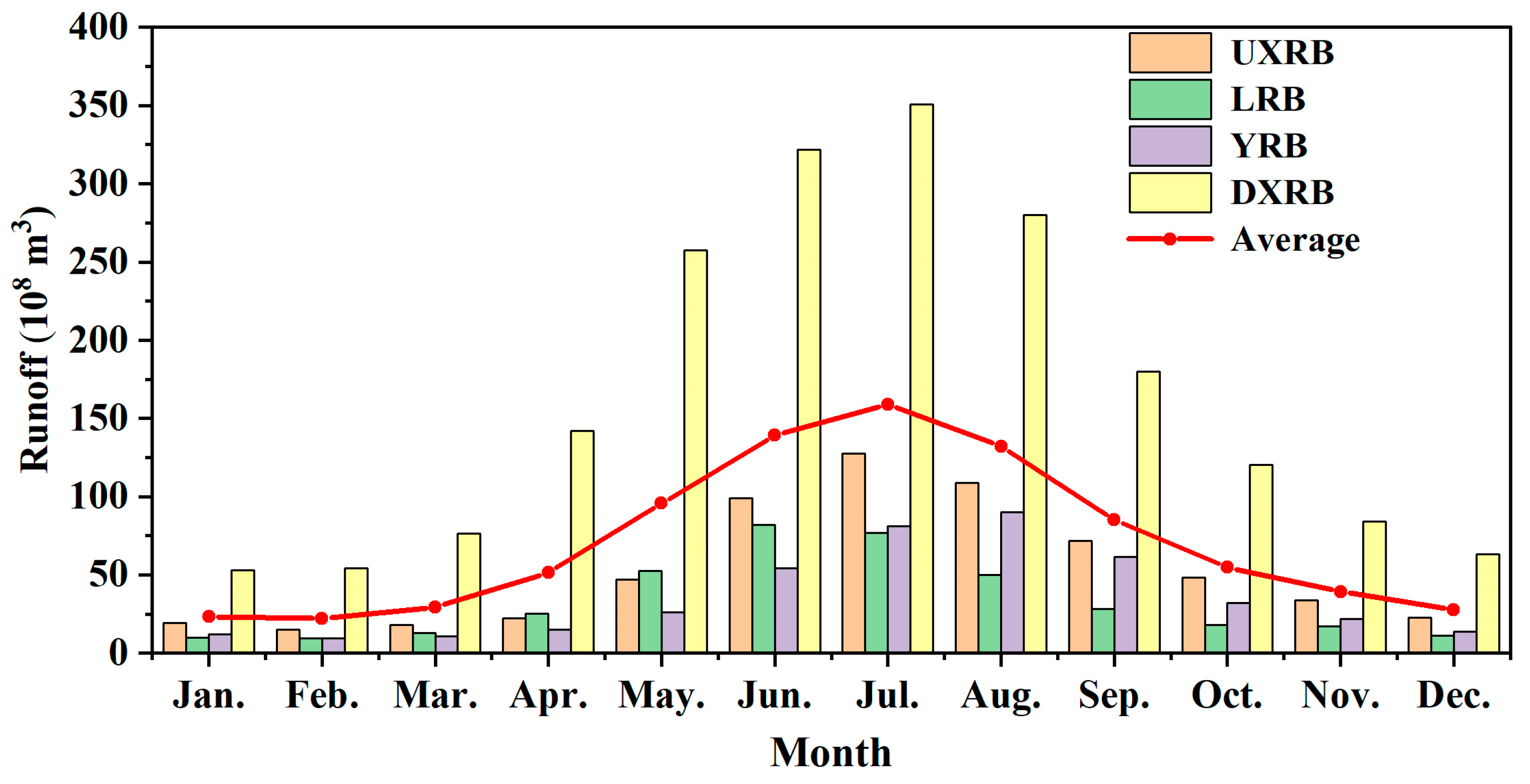
4.1. Analysis of Monthly Runoff Evolution

The monthly runoff evolution of each sub-basin in the XRB from 1961 to 2020 are illustrated in Figure 2. The runoff changes in the four sub basins are small from January to March, with the smallest average runoff of 21.96 × 10⁸ m³ occurring in February. From April, the runoff in each sub basin increases rapidly, reaching its maximum monthly average of 159.08 × 10⁸ m³ in July, followed by a gradual decline from August to December, reaching a minimum value of 27.57 × 10⁸ m³ in December. Overall, the DXRB has a larger multi-year average monthly runoff value, reaching 165.19 × 10⁸ m³. As for the evolution pattern of dry-season runoff shown in Figure 2, the characteristics of runoff changes during the dry season in the XRB and each sub-basin are generally consistent. With the onset of winter, precipitation decreases continuously from October to February of the following year. The multi-year average monthly runoff is 54.67 × 10⁸ m³ in October, and February marks the month with the minimum runoff during the dry season, with an average monthly runoff of only 21.96 × 10⁸ m³. Subsequently, runoff gradually increases from February to March, with the annual average runoff rising to 29.35 × 10⁸ m³ in March. Similarly, the highest amount of dry-season runoff (450.63 × 10⁸ m³) occurs in the DXRB.

Table 3. Annual and dry-season runoff characteristics of various sub-basins in the XRB.

Sub-Basins	Whole Year		Dry Season		Dry-Season Runoff/Whole Year Runoff (%)
	Runoff (108 m3)	Coefficient of Variation	Runoff (108 m3)	Coefficient of Variation
UXRB	633.32	0.23	156.42	0.27	24.7
LRB	392.33	0.23	77.67	0.33	19.8
YRB	428.39	0.32	100.15	0.34	23.4
DXRB	1982.29	0.20	450.63	0.26	22.7

shows the annual and dry-season runoff characteristics for each sub-basin in the XRB from 1961 to 2020. According to Table 3, the annual average runoff for the UXRB, LRB, YRB, and DXRB are 633.32 × 10⁸ m³, 392.33 × 10⁸ m³, 428.39 × 10⁸ m³, and 1982.29 × 10⁸ m³, respectively. The highest coefficient of variation is found in the YRB, with a value of 0.32. The DXRB receives runoff from several sources, including the Xijiang, Liujiang, and Yujiang Rivers, leading to a relatively high runoff. During the dry season, the LRB has the smallest annual average runoff, at 77.67 × 10⁸ m³, with a coefficient of variation of 0.33. Additionally, the ratio of dry-season runoff to annual runoff varies across different sub-basins. The UXRB has a dry-season runoff of 156.42 × 10⁸ m³, accounting for 24.7% of the total annual runoff.

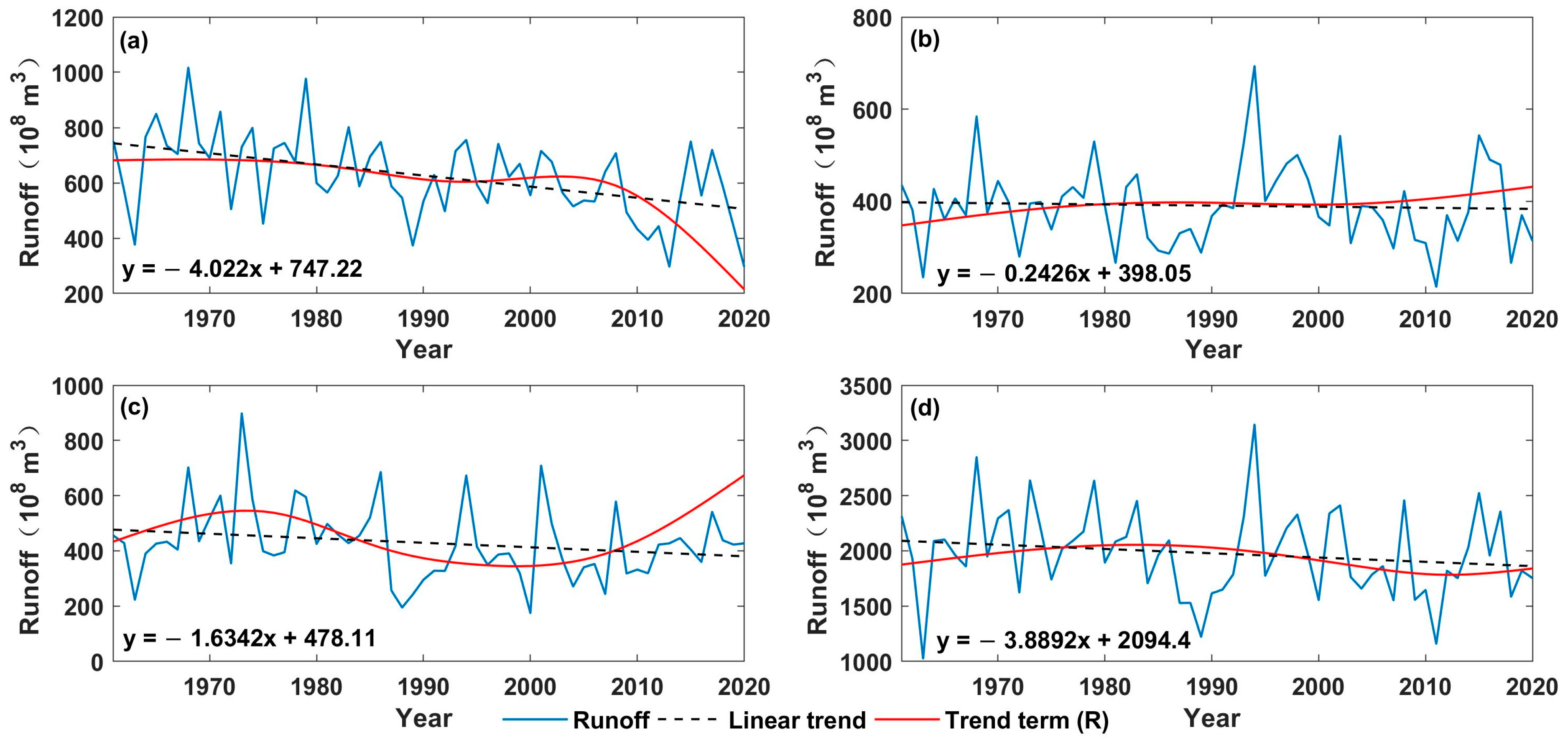
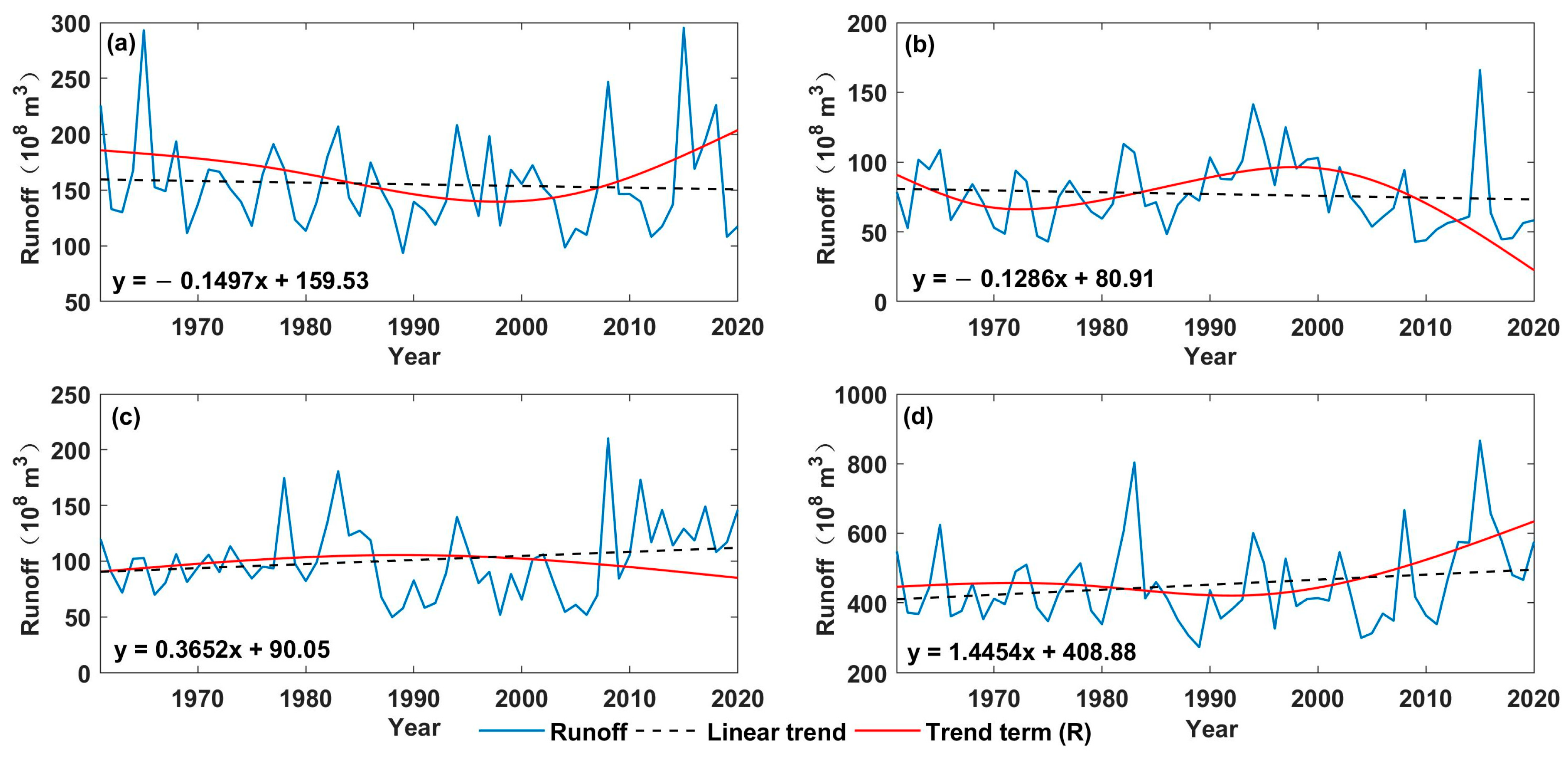
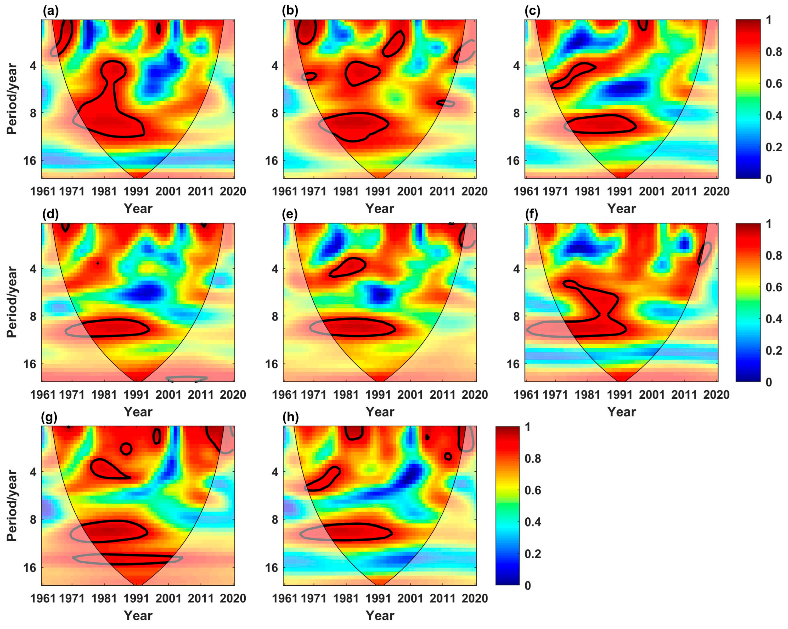
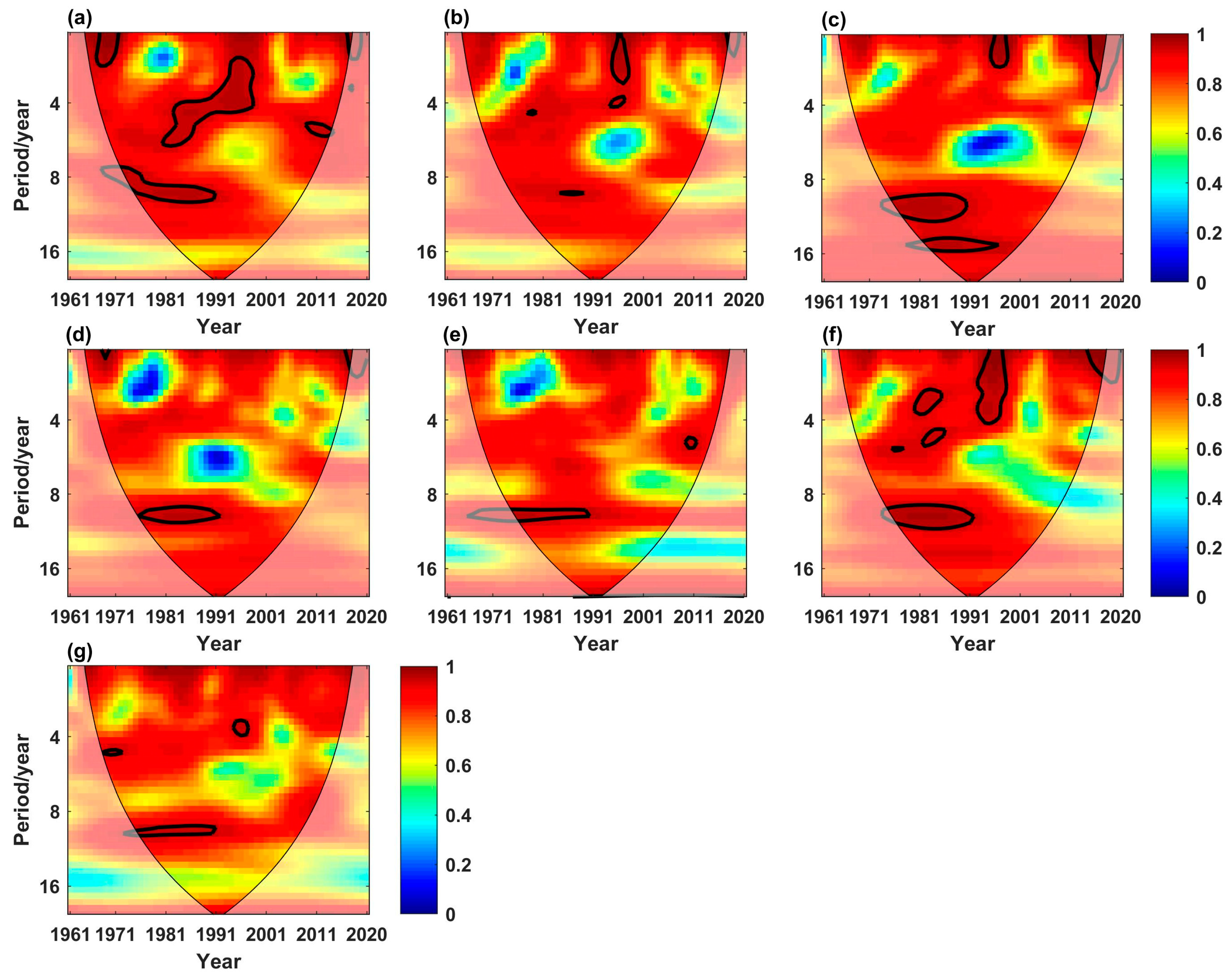
4.2. Identification of Trends, Periodicity, and Variability

This study employs the ESMD method to analyze the runoff data from four sub-basins in the XRB from 1961 to 2020. After multiple screenings of the decomposition process, the optimal number (seven times) of screenings is determined, and the decomposition is automatically stopped based on this criterion. Throughout this process, the proportion of variance attributed to the R is minimized, leading to the decomposition results of the IMF components and one R. As shown in

Table 4. Periods, variance contribution rates, and correlation coefficients of each component in the annual runoff series of the XRB.

Sub-Basins	IMF Component	IMF1	IMF2	IMF3	IMF4	R
UXRB	Period (year)	2.90	9.67	14.50	29.00
	Variance contribution rate (%)	37.41	22.14	13.73	4.76	21.96
	Correlation coefficient	0.58 **	0.42 **	0.26	0.19	0.32 *
LRB	Period (year)	2.90	7.25	11.60	29.00
	Variance contribution rate (%)	41.90	25.37	25.85	4.11	2.77
	Correlation coefficient	0.60 **	0.43 **	0.48 **	0.13	0.10
YRB	Period (year)	3.87	8.29	29.00	\
	Variance contribution rate (%)	39.28	36.14	9.48	\	15.10
	Correlation coefficient	0.49 **	0.48 **	0.14	\	0.38 **
DXRB	Period (year)	3.75	6.67	15.00	30.00
	Variance contribution rate (%)	51.50	22.05	10.38	11.46	4.61
	Correlation coefficient	0.67 **	0.42 **	0.25	0.35 **	0.12

Note: “*” and “**” denote significant at 0.05 and 0.01 level, respectively.

; the average periods of each modal component are calculated using the fast Fourier transform and the periodogram method. The variance contribution rate is used to indicate the frequency and amplitude of annual-scale signal fluctuations’ impact on the overall characteristics of the original data. Clearly, the variance contribution rates of IMF1 components for each sub-basin are the highest, at 37.41%, 41.90%, 39.28%, and 51.50%, respectively, with correlation coefficients of 0.58, 0.60, 0.49, and 0.67 with the original runoff series, all passing the significance test at α = 0.01. Regarding the average period, the periods of the first two IMF components are less than 10 years. The DXRB exhibits periodic characteristics of 3.75 and 6.67 years on an interannual scale and 15 and 30 years on an interdecadal scale.

Following ESMD decomposition, the R of runoff sequences from various sub-basins in the XRB is depicted in Figure 3, with panels (a)–(d) representing the UXRB, LRB, YRB, and DXRB, respectively. From Figure 3, it is observed that the runoff sequence of the UXRB exhibits a steady declining trend throughout the entire time series, with a linear trend rate of −40.22 × 10⁸ m³/10a. The runoff sequence of the LRB shows a gradual increase from 1961 to 1994, followed by a gradual decrease from 1995 to 2020. The runoff sequence of the YRB shows an upward trend from 1961 to 1973, a slow decline from 1974 to 2000, and a slight increase from 2001 to 2020. The runoff sequence of the DXRB demonstrates a slow declining trend, with a linear trend rate of −38.89 × 10⁸ m³/10a. These results indicate a general decrease in runoff throughout the XRB, attributed to the frequent occurrence of droughts under the coupled effects of climate change and human activities in the 21st century, exhibiting a trend towards warmer and drier conditions.

Figure 4 illustrates the dynamic variations in runoff volume in the XRB from 1961 to 2020 based on the BEAST algorithm. Notably, gray enveloping intervals around the change-point times, as well as light-shaded areas surrounding the fitted trend and seasonal curves, represent their 95% confidence intervals. The seasonal component of runoff in the XRB exhibits periodic fluctuations, with peaks and troughs alternating. The maximum occurs in July, with a mean of 350.64 × 10⁸ m³, while the minimum appears in January, averaging 52.75 × 10⁸ m³. Seasonal change-points in runoff volume are typically induced by the periodic variation in precipitation. Overall, the probability of a seasonal change-point occurring is 66.3% in April 2002, with a confidence interval spanning from August 2001 to February 2003. The mean runoff volumes are 168.56 × 10⁸ m³ and 156.83 × 10⁸ m³ before and after this change-point, respectively. Furthermore, trend change-points generally signify a transition in runoff dynamics from one climatic pattern to another, reflecting trends of stability, increase, or decrease in runoff. For the XRB, there is a 30.2% probability of one trend change-point, occurring in July 1983. The confidence interval for this change-point spans from March 1980 to May 1985, with mean runoff volumes before and after of 175.19 × 10⁸ m³ and 158.81 × 10⁸ m³, respectively. Meanwhile, this change-point is classified as an interrupted increase. Additionally, identified harmonic orders also undergo changes before and after change-points, enhancing their application in runoff change detection.

4.3. Runoff Variation Characteristics during the Dry Season

Using the ESMD decomposition method,

Table 5. Periods, variance contribution rates, and correlation coefficients of each component in the dry-season runoff series of the XRB.

Sub-Basins	IMF Component	IMF1	IMF2	IMF3	IMF4	IMF5	R
UXRB	Period (year)	3.53	7.50	15.00	30.00	\
	Variance contribution rate (%)	43.46	35.76	3.06	4.73	\	13.00
	Correlation coefficient	0.66 **	0.40 **	0.12	0.12	\	0.18
LRB	Period (year)	4.29	8.57	20.00	\	\
	Variance contribution rate (%)	39.12	25.84	12.28	\	\	22.76
	Correlation coefficient	0.39 **	0.28 *	0.28 *	\	\	0.36 **
YRB	Period (year)	2.31	8.57	15.00	30.00	30.00
	Variance contribution rate (%)	36.58	23.14	13.84	25.86	0.31	0.27
	Correlation coefficient	0.60 **	0.45 **	0.28 *	0.49 **	0.17	0.06
DXRB	Period (year)	4.29	8.57	15.00	20.00	30.00
	Variance contribution rate (%)	30.63	33.98	5.85	3.48	6.92	19.14
	Correlation coefficient	0.50 **	0.31 *	0.13	0.17	0.28 *	0.44 **

Note: “*” and “**” denote significant at 0.05 and 0.01 level, respectively.

presents the periodic components, variance contribution rates, and correlation coefficients of dry-season runoff in various sub-basins of the XRB from 1961 to 2020. In the UXRB, the variability of dry-season runoff can be decomposed into four IMF components and one R. The periods of these components are 3.53 years, 7.5 years, 15 years, and 30 years, indicating the periodic characteristics of 3.53 and 7.5 years on an interannual scale and 15 and 30 years on an interdecadal scale in runoff variations. The variance contribution rates are 43.46%, 35.76%, 3.06%, and 4.73%, respectively. Additionally, IMF1 exhibits the highest correlation with the original series, with a coefficient of 0.66 (p < 0.01). In other sub-basins, the maximum variance contribution rates are all found in the IMF1 component, with values of 39.12%, 36.58%, and 30.63%, respectively (p < 0.01).

Figure 5 illustrates the trends of dry-season runoff in various sub-basins of the XRB based on the ESMD decomposition, with (a)–(d) representing the UXRB, LRB, YRB, and DXRB, respectively. It is observed from Figure 5 that the dry-season runoff in the UXRB and LRB shows a slight decreasing trend, with linear trends of −1.497 × 10⁸ m³/10a and −1.286 × 10⁸ m³/10a, respectively. The maximum dry-season runoff in the UXRB (295.41 × 10⁸ m³) occurred in 2015, while the minimum (93.47 × 10⁸ m³) occurred in 1989; for the LRB, the maximum (165.99 × 10⁸ m³) occurred in 2015, and the minimum (42.72 × 10⁸ m³) occurred in 2009. In contrast, the dry-season runoff in the YRB and DXRB shows an increasing trend, with linear trends of 3.652 × 10⁸ m³/10a and 14.454 × 10⁸ m³/10a, respectively. The maximum dry-season runoff in the YRB occurred in 2008 (210.24 × 10⁸ m³), while the minimum occurred in 1988 (49.81 × 10⁸ m³); for the DXRB, the maximum occurred in 2015 (866.41 × 10⁸ m³), and the minimum occurred in 1989 (273.93 × 10⁸ m³).

Figure 6 presents the dynamic characteristics of dry-season runoff in the XRB from 1961 to 2020 based on the BEAST algorithm. The seasonal components of dry-season runoff in the XRB exhibit periodic variations, with the maximum occurring in 2015 and the minimum in 1989. Overall, the probability of a seasonal change point is 20.5% in dry-season runoff, occurring in 1983 with a confidence interval from 1980 to 1986, and the mean dry-season runoff is 454.57 × 10⁸ m³ and 451.97 × 10⁸ m³ before and after this change point, respectively. The probability of a trend change point is 70.5% in 2013, with a confidence interval from 2010 to 2015. The mean dry-season runoff before and after this change point is 433.64 × 10⁸ m³ and 599.33 × 10⁸ m³, respectively, and the type of change point is a monotonic increase.

4.4. The Driving Force of Circulation Factors

Figure 7 presents the wavelet coherence power spectrum for the annual dry-season runoff and atmospheric circulation factors in the low-energy zone during 1961–2020 across the XRB. Analysis of the resonance between runoff and ENSO reveals two significant positive correlation periods: a 4–6 years cycle observed during 1971–1981 and a 1–4 years cycle during 1991–2000. Examination of the resonance between runoff and PDO indicates two significant positive correlation periods: a 15–20 years cycle observed from 1981 to 2001 and a 1–2 years cycle from 1995 to 2000. Analysis of the resonance between runoff and AO reveals four significant positive correlation periods: a 1–4 years cycle during 1965–1972, an 8–9 years cycle from 1982 to 1992, a 1–2 years cycle in 1995–2001, and a 6–8 years cycle from 2003 to 2012. Resonance analysis between runoff and AMO indicates three significant negative correlation periods: a 1–2 years cycle from 1966 to 1971, an 8–9 years cycle during 1976–1982, and a negative correlation period of 3–4 years from 1978 to 1993.

Additionally, periodic resonance analysis between runoff and DMI reveals two significant positive correlation periods: a 4–6 years cycle observed during 1978–1987 and a 1–5 years cycle from 1992 to 2001. Periodic resonance analysis between runoff and NPI indicates three significant correlation periods: a positive correlation cycle of 1–4 years from 1985 to 2001, a negative correlation cycle of 16–18 years from 1985 to 1995, and a negative correlation cycle of 1–3 years from 2008 to 2011. Periodic resonance analysis between runoff and PNA reveals one significant positive correlation period from 1983 to 2000, with a cycle of 1–3 years. Periodic resonance analysis between runoff and SSI indicates one significant negative correlation period from 1972 to 2001, with a cycle of 8–12 years.

Figure 8 illustrates the cross-wavelet transform graph in high-energy region of annual dry-season runoff and corresponding atmospheric circulation factors in the XRB from 1961 to 2020. The color bars represent the wavelet power spectrum, where higher values indicate stronger signal oscillations and more significant confidence in the period’s significance test. It is evident from the figure that during 1972–2006, there is a significant negative correlation resonance period of 8–14 years between dry-season runoff and SSI, indicating the strongest impact of SSI on dry-season runoff and the negative correlation. Apart from the SSI, the ENSO also significantly influences the dry-season runoff, exhibiting a 2–6 years cycle from 1976 to 1990 and a 6–8 years cycle from 2001 to 2012, both showing positive correlations.

Figure 9 shows the multiple wavelet coherence of different circulation factors on the runoff-SSI in the XRB. Obviously, the maximum values of AWC and POSP coupled with two factors appear in the SSI-ENSO combination, with values of 0.95 and 18.68%, respectively, indicating that the bivariate influencing factors SSI and ENSO both play dominant roles in the process of runoff variation (

Table 6. The AWC and POSP values between runoff and climate variables (ENSO, PDO, NAO, AO, AMO, DMI, NPI, PNA and SSI) based on multiple wavelet coherence.

Univariate	AWC	POSP (%)	Bivariate	AWC	POSP (%)	Trivariate	AWC	POSP (%)
ENSO	0.92	12.98	SSI-ENSO	0.95	18.68	SSI-ENSO-PDO	0.97	20.13
PDO	0.92	11.47	SSI-PDO	0.94	15.74	SSI-ENSO-NAO	0.94	14.63
NAO	0.90	2.43	SSI-NAO	0.93	10.41	SSI-ENSO-AO	0.95	15.62
AO	0.91	6.87	SSI-AO	0.92	8.54	SSI-ENSO-AMO	0.95	15.48
AMO	0.91	5.03	SSI-AMO	0.93	11.54	SSI-ENSO-DMI	0.95	16.21
DMI	0.91	5.64	SSI-DMI	0.93	10.78	SSI-ENSO-NPI	0.96	18.67
NPI	0.92	9.67	SSI-NPI	0.94	14.20	SSI-ENSO-PNA	0.95	16.78
PNA	0.92	9.45	SSI-PNA	0.93	9.63
SSI	0.93	13.42

). Overall, there are two resonance periods between runoff and SSI-ENSO, which are 1–4 years (1963–1971) and 4–12 years (1971–1991), respectively.

Among the three variable combinations, SSI-ENSO-PDO has the greatest impact on runoff (Figure 10). At this time, the AWC and POSP values are 0.97 and 20.13%, respectively. There are four resonance periods between runoff and SSI-ENSO-PDO, namely, 1–2 years (1968–1971), 7–12 years (1969–1990), 2–6 years (1981–2000), and 5–6 years (2008–2011). Therefore, the best three-factor combination that can well explain the changes in runoff during the dry season is SSI-ENSO-PDO in the XRB.

5. Discussion

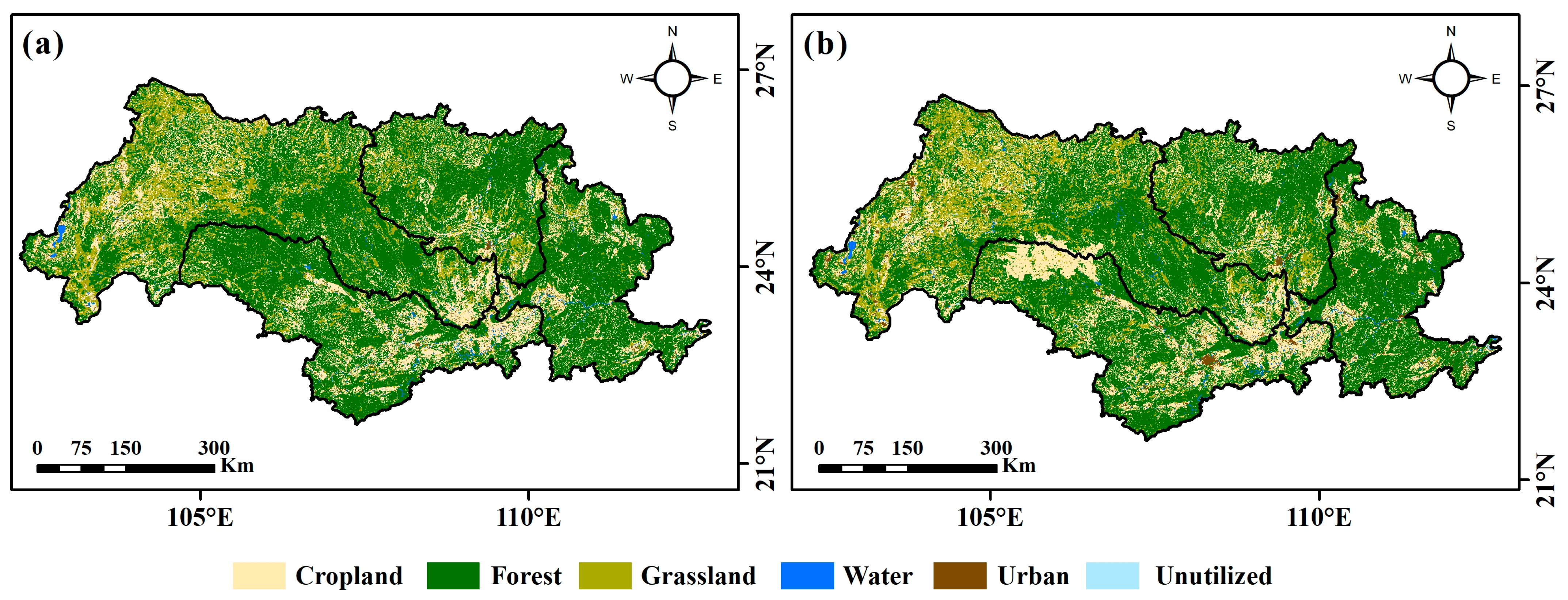
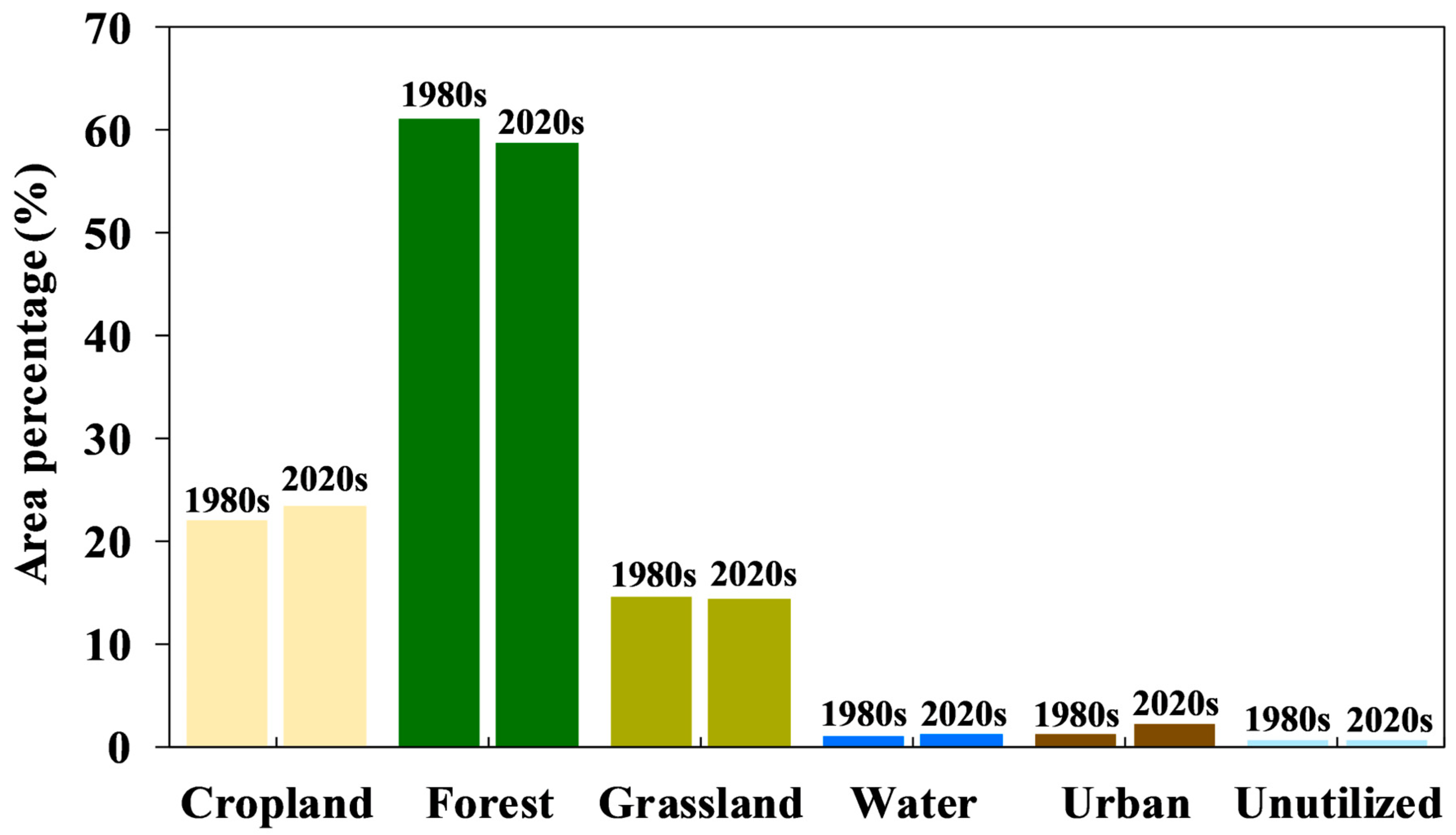
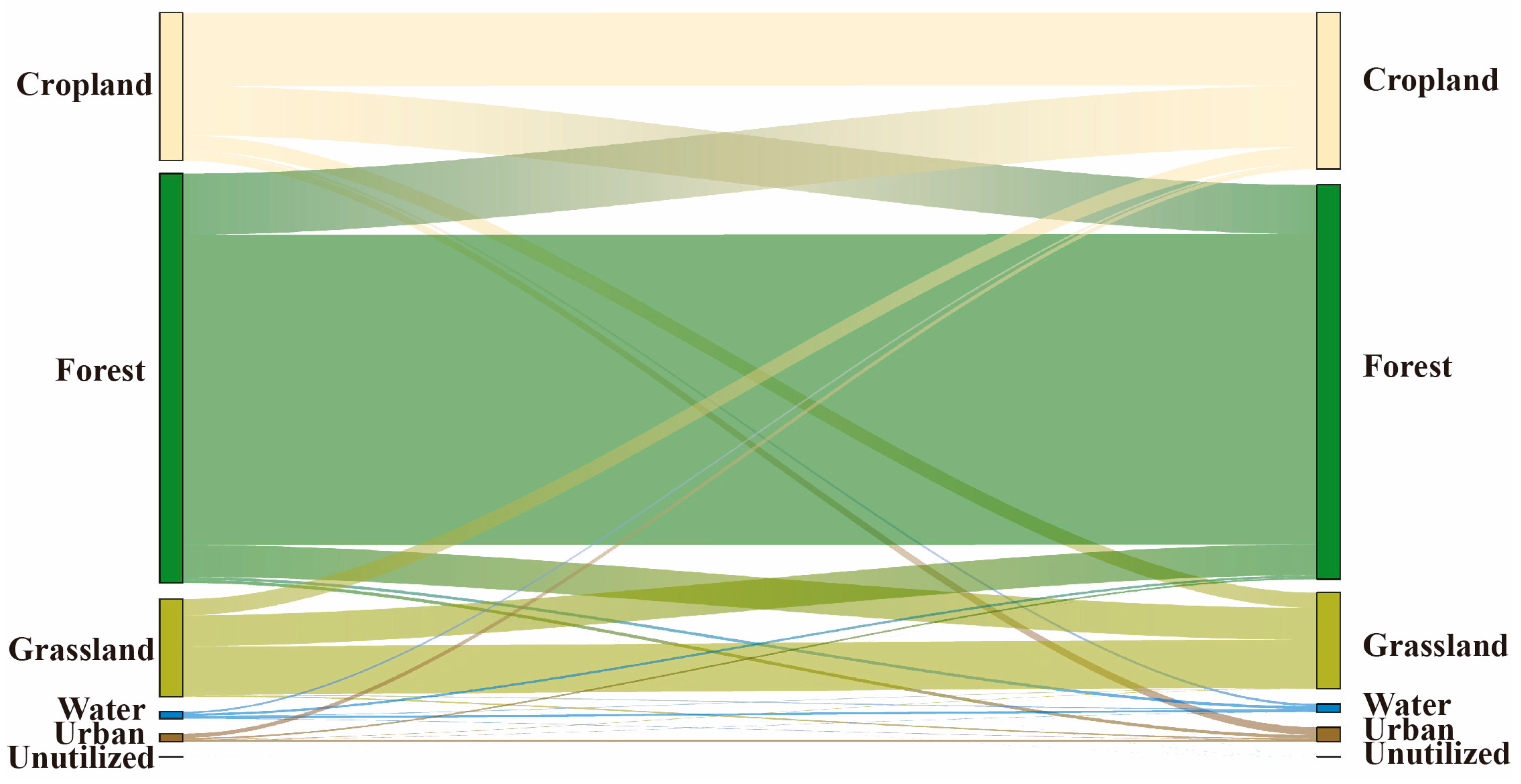
5.1. The Impact of Land Use on Runoff

Land use is one of the primary factors influencing the water cycle, and runoff variation constitutes a crucial component of the water cycle [53]. Consequently, changes in land use have significant impacts on runoff, altering natural precipitation mechanisms and influencing hydrological processes within watersheds [54,55]. Since the emergence of remote sensing technology in the 1980s, it has provided a valuable tool for assessing land use. Land use data from 1980 to 2020 were selected to investigate the influence of land use changes on runoff (Figure 11). Figure 12 denotes the area percentage of land use across the XRB in the 1980s and 2020s. In the XRB, forests are the predominant land use type, covering over half of the study area, mainly concentrated in the eastern part of the basin. Specifically, the percentage of forest area was 61.12% in the 1980s and 58.84% in the 2020s. Additionally, cropland and grassland are also major land use types, with average area percentages of 22.69% and 14.45%, respectively. During the study period, cropland, water bodies, and urban land in the XRB showed an increasing trend, while the areas of other land use types (forests, grasslands, unutilized land) decreased. Among them, the forest area decreased by 7584 km², accounting for approximately 2.27% of the study area.

As shown in Figure 13, the increase in cropland area primarily resulted from the conversion of forest (30,434 km²) and grassland (8057 km²). The expansion of water bodies mainly came from cropland (1168 km²) and forest (1436 km²). Similarly, a portion of cropland (3861 km²) and forest (1589 km²) was transformed into urban land. These changes in land use structure directly affect the watershed’s surface conditions, which are associated with the runoff generation and routing processes, ultimately influencing hydrological characteristics [31,32]. During the study period, the areas of urban land, water bodies, and unutilized land showed positive correlations with dry-season runoff, with correlation coefficients of 0.58, 0.51, and 0.42, respectively. Overall, the increase in urban land area had the most significant impact on runoff. Urban expansion hinders water infiltration, leading to reduced rainwater percolation and declining groundwater levels. This not only increases the runoff coefficient but also accelerates the flow process and increases runoff volume [56]. Additionally, the increase in forest area may contribute to a reduction in runoff volume [57].

5.2. Advantages and Limitations

Under the combined influence of changing climate conditions and escalating human activities, the river runoff in the XRB has undergone varying degrees of changes [5,43]. In recent decades, there has been a decreasing trend in runoff in the XRB, consistent with the findings of Niu et al. [9]. In the XRB, the 1970s and 1990s experienced relatively abundant runoff, while the 2010s marked the period of lowest runoff [58]. After multiple iterations of training, ESMD can be used to reflect the overall fluctuation of runoff [59]. Examining the non-linear trends in a time series perspective, we not only detected the non-monotonic trends in the full-time series and the dry-season runoff time series but also analyzed the abrupt change processes in trend components and seasonal components. While studying the stage specific details of long-term runoff changes, attention was also paid to possible abrupt changes and trend transitions (Figure 4). Unlike traditional change point detection algorithms, BEAST considers the error range of the model to obtain the probability of change occurring at any given time point [50,60]. One of the advantages of BEAST is that it assumes that all unknowns are random variables, clearly describing various uncertainties [61]. It is noteworthy that Tian et al. [41] also identified 1983 as a turning year for the dry and wet conditions in the XRB. Climate change, construction of water conservancy projects, and changes in land use could all be reasons for runoff changes [1,3]. Regional environmental factors such as precipitation and evapotranspiration may affect runoff variations. Also, we calculated the correlation coefficients between precipitation, evapotranspiration, and dry-season runoff in this region and found that the correlation coefficients were 0.68 (p < 0.01) and 0.63 (p < 0.01), respectively. Given that the p-value is less than 0.01, we have sufficient evidence to reject the null hypothesis and consider the observed results to be statistically significant. Therefore, both precipitation and evapotranspiration have a significant impact on the dry-season runoff in the XRB, and the driving force of precipitation is slightly higher than that of evapotranspiration.

Based on the cross-wavelet transform technique, it was found that different atmospheric circulation factors have varying driving effects on dry-season runoff changes (Figure 8). The cross-wavelet analysis has unveiled significant correlations between dry-season runoff and various atmospheric circulation factors. For instance, the sunspot activity, as indicated by the SSI, has been linked to climatic impacts due to its magnetic field variations, which could influence precipitation patterns and consequently runoff in the XRB [34,62]. Furthermore, the ENSO and PDO, known for their influence on large-scale oceanic circulation, have been identified to modulate the hydrological cycle, affecting the runoff dynamics through altered precipitation and evaporation rates. In the present study, the multiple wavelet coherence is useful and important as it can simultaneously evaluate the impact of multiple circulation factors at different time scales [63]. In addition, ENSO and PDO also have an obvious impact on the runoff changes in the XRB (Figure 10). Lin et al. [40] and Tian et al. [41] demonstrated that the long-term seasonality and spatial variation of ENSO intensity are related to the fluctuations of precipitation, which also supports our research results. For PDO, it is one of the important internal variables of climate systems that cause changes in runoff and has a good ability to predict runoff [51]. As sunspots, ENSO, and PDO are the important external energy inputs and influencing factors for dry-season runoff changes, they can be used as input factors for predicting dry-season runoff in the XRB to improve runoff forecasting accuracy in the future.

There are still some limitations. During time domain expansion, wavelet images require complex meteorological interpretations [52,64]. Furthermore, human activities also alter hydrological conditions and affect runoff, for example, the construction of reservoirs to regulate runoff, the construction of water supply projects from the river water, large-scale irrigation water consumption, and so on. The data on hydropower installation and development have not been effectively collected, which may be one of the limitations of this study. Hydropower development can improve its utilization efficiency by regulating the temporal and spatial distribution of water resources. When conducting hydrological modeling in the study area, land use models should consider the impact of human intervention (such as reservoir operation). Therefore, the impact of human activities should be given due consideration [65,66].

5.3. Future Prospects

In the future, our research will delve into several key aspects. First, accurate prediction of runoff during the dry season holds significant importance for scientific and precise water management. Based on our identification of the trends and periodicity in dry-season runoff, policymakers should consider the variability of water resources on both long-term and seasonal bases and formulate flexible water allocation plans. Our finding of a negative correlation between sunspot activity and dry-season runoff underscores the importance of climatic factors in water resource management, which needs to be taken into account when formulating policies. The findings of this study can provide informational support for real-time water resource management and planning in the XRB. Furthermore, our analysis of the coupling effects between atmospheric circulation factors and the dynamics of runoff variations can assist in real-time monitoring and adjustment of water resource management strategies to adapt to the impacts of climate change. Establishing hydrological models tailored to the XRB can offer reliable insights into forecasting dry-season runoff [5,55,67]. Second, storing a portion of water during the wet season to supplement the inadequacy of water during the dry season serves as an effective measure to alleviate water scarcity. The presence of numerous lakes and low-lying areas along riverbanks provides favorable conditions for harnessing basin rainwater resources, could enhance water supply guarantee during the dry season [68]. Lastly, it is imperative to gather multi-source basin data to generate high-quality, continuous, meteorological-driven and human activity-related data, such as actual water consumption and reservoir operations, which will accurately depict the impact of human activities on runoff [31,32].

6. Conclusions

This study identifies the trend and periodic characteristics of runoff in the XRB from 1961 to 2020, analyzes the dynamic variations of dry-season runoff, and reveals the driving role of atmospheric circulation factors in the dynamic changes of dry-season runoff. The following conclusions can be drawn:

(1)

During the research period, the characteristics of runoff changes were generally consistent during the dry season in the XRB and each sub-basin. The minimum and maximum monthly runoff occurred in February and October, respectively. On an interannual scale, dry-season runoff exhibited periodicity of 3.53 years and 7.5 years.

(2)

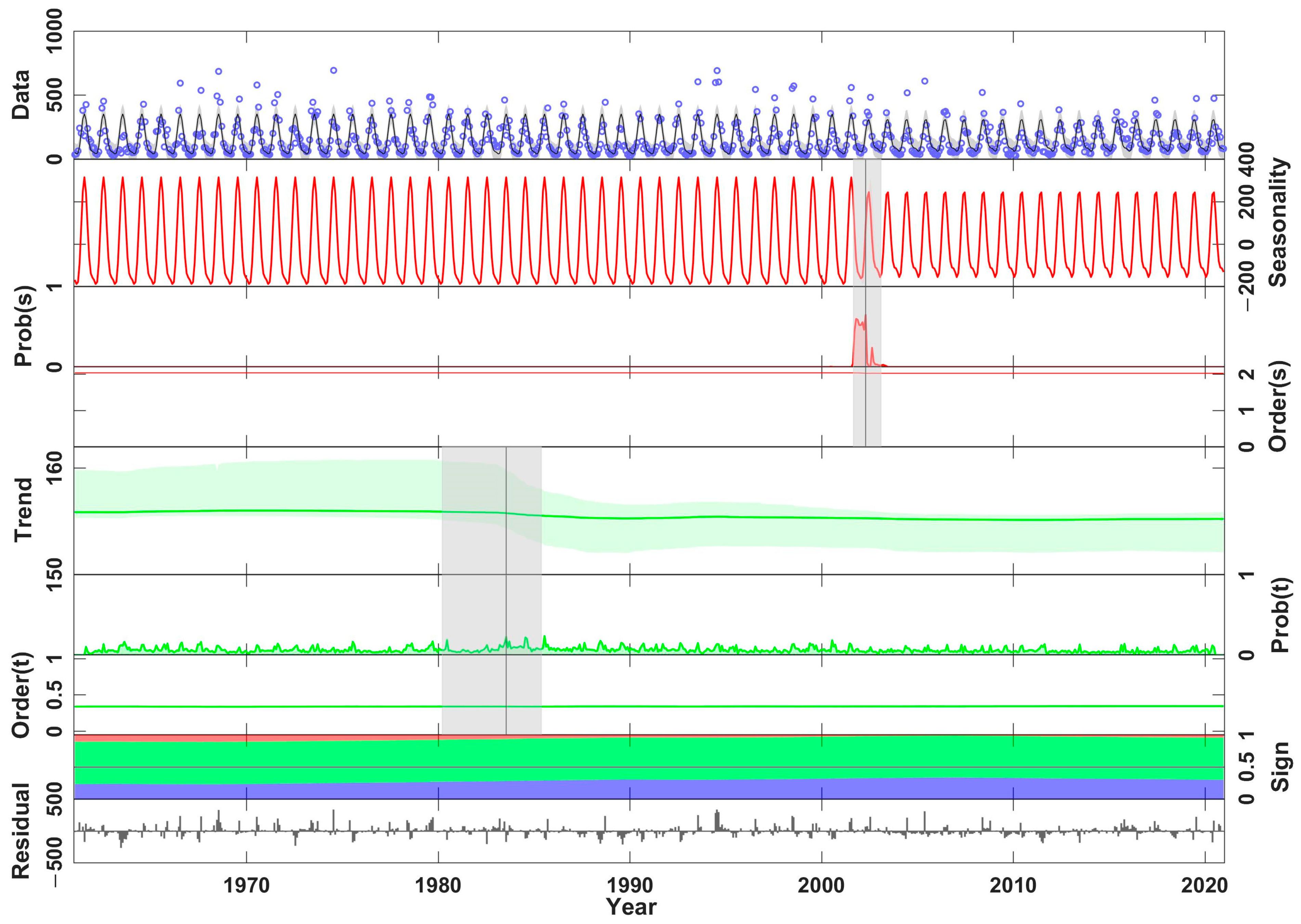
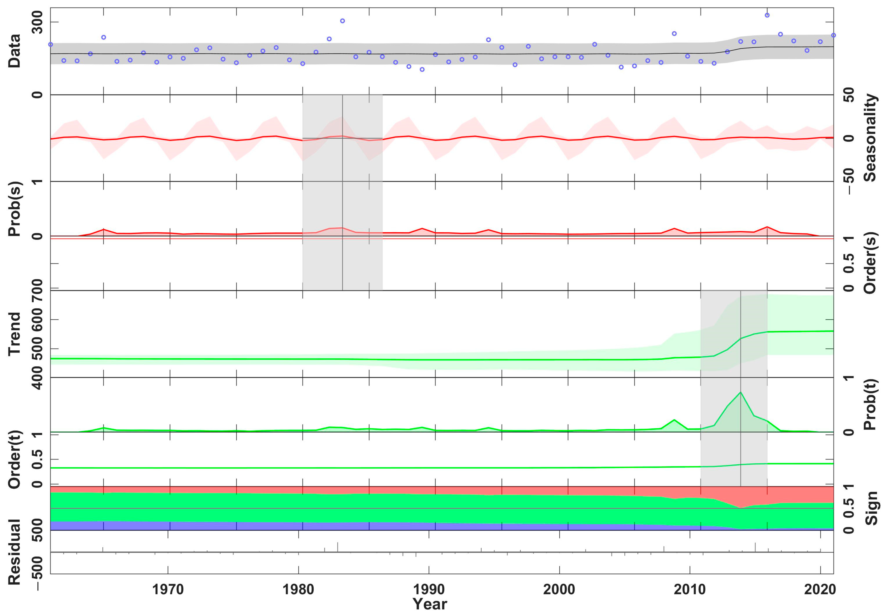
Based on the BEAST algorithm, the seasonal abrupt point occurred in 1983, with a confidence interval from 1980 to 1986. Additionally, the trend abrupt point occurred in 2013, with a confidence interval from 2010 to 2015.

(3)

The evolution characteristics of dry-season runoff in the XRB were significantly influenced by atmospheric circulation anomaly factors. Overall, SSI-ENSO-PDO had the greatest impact on the changes in dry-season runoff in the XRB.

(4)

Land use change has had an impact on runoff in the XRB. Specifically, the increase in urban land area had an obvious impact on runoff. In addition, an increase in forest area may contribute to a decrease in runoff.

(5)

Based on seasonal and long-term trends of runoff, water resource allocation policies can be proposed. Advanced hydrological models and remote sensing technology can be utilized to improve the accuracy of dry-season runoff prediction and provide scientific basis for real-time water resource management.

References

1. Risva, K.; Nikolopoulos, D.; Efstratiadis, A.; Nalbantis, L. A Framework for Dry Period Low Flow Forecasting in Mediterranean Streams. Water Resour. Manag. 2018, 32, 4911–4932. [Google Scholar] [CrossRef]
2. Li, Z.J.; Liu, M.Q.; Li, Z.X.; Feng, Q.; Song, L.L.; Xu, B.; Liu, X.Y.; Gui, J. Where does the runoff come from in dry season in the source region of the Yangtze River? Agr. For. Meteorol. 2023, 330, 109314. [Google Scholar]
3. Singh, R.; Mishra, V. Atmospheric and Land Drivers of Streamflow Flash Droughts in India. J. Geophys. Res.-Atmos. 2024, 129, e2023JD040257. [Google Scholar] [CrossRef]
4. Duan, Y.; Xu, G.B.; Liu, Y.; Liu, Y.J.; Zhao, S.X.; Fan, X.L. Tendency of Runoff and Sediment Variety and Multiple Time Scale Wavelet Analysis in Hongze Lake during 1975–2015. Water 2020, 12, 999. [Google Scholar] [CrossRef]
5. Lin, Q.X.; Wu, Z.Y.; Zhang, Y.L.; Peng, T.; Chang, W.J.; Guo, J.L. Propagation from meteorological to hydrological drought and its application to drought prediction in the Xijiang River basin, South China. J. Hydrol. 2023, 617, 128889. [Google Scholar] [CrossRef]
6. Jiang, K.; Mo, S.; Yu, K.; Li, P.; Li, Z. Analysis on the relationship between runoff erosion power and sediment transport in the Fujiang River basin and its response to land use change. Ecol. Indic. 2024, 159, 111690. [Google Scholar] [CrossRef]
7. Bing, L.F.; Shao, Q.Q.; Liu, J.Y. Runoff characteristics in flood and dry seasons based on wavelet analysis in the source regions of the Yangtze and Yellow rivers. J. Geogr. Sci. 2012, 22, 261–272. [Google Scholar] [CrossRef]
8. Mallakpour, I.; Sadegh, M.; AghaKouchak, A. A new normal for streamflow in California in a warming climate: Wetter wet seasons and drier dry seasons. J. Hydrol. 2018, 567, 203–211. [Google Scholar] [CrossRef]
9. Niu, J.; Chen, J.; Sun, L.Q. Exploration of drought evolution using numerical simulations over the Xijiang (West River) basin in South China. J. Hydrol. 2015, 526, 68–77. [Google Scholar] [CrossRef]
10. Smakhtin, V.U. Low flow hydrology: A review. J. Hydrol. 2001, 240, 147–186. [Google Scholar] [CrossRef]
11. Guan, B.T.; Wright, W.E.; Chiang, L.H.; Cook, E.R. A dry season streamflow reconstruction of the critically endangered Formosan landlocked salmon habitat. Dendrochronologia 2018, 52, 152–161. [Google Scholar] [CrossRef]
12. Tian, J.X.; Chang, J.; Zhang, Z.X.; Wang, Y.J.; Wu, Y.F.; Jiang, T. Influence of Three Gorges Dam on Downstream Low Flow. Water 2019, 11, 65. [Google Scholar] [CrossRef]
13. Wang, F.E.; Xie, X.H. Practice and thinking on “Three Defense Lines” of water supply system regulation in the Pearl River Basin during 2022–2023 dry season. China Flood Drought Manag. 2024, 34, 32–35. [Google Scholar]
14. Palmer, T.A.; Montagna, P.A. Impacts of droughts and low flows on estuarine water quality and benthic fauna. Hydrobiologia 2015, 753, 111–129. [Google Scholar] [CrossRef]
15. Wang, W.Z.; Dong, Z.C.; Zhu, F.L.; Cao, Q.; Chen, J.; Yu, X. A Stochastic Simulation Model for Monthly River Flow in Dry Season. Water 2018, 10, 1654. [Google Scholar] [CrossRef]
16. Cingolani, A.M.; Poca, M.; Whitworth-Hulse, J.I.; Giorgis, M.A.; Vaieretti, M.V.; Herrero, L.; Ramos, S.N.; Renison, D. Fire reduces dry season low flows in a subtropical highland of central Argentina. J. Hydrol. 2020, 590, 125538. [Google Scholar] [CrossRef]
17. Mosley, L.M.; Zammit, B.; Leyden, E.; Heneker, T.M.; Hipsey, M.R.; Skinner, D.; Aldridge, K.T. The Impact of Extreme Low Flows on the Water Quality of the Lower Murray River and Lakes (South Australia). Water Resour. Manag. 2012, 26, 3923–3946. [Google Scholar] [CrossRef]
18. Zhou, Z.; Ouyang, Y.; Qiu, Z.; Zhou, G.; Lin, M.; Li, Y. Evidence of climate change impact on stream low flow from the tropical mountain rainforest watershed in Hainan Island, China. J. Water Clim. Chang. 2017, 8, 293–302. [Google Scholar] [CrossRef]
19. Wu, G.D.; Zhang, J.Y.; Li, Y.L.; Ren, H.Z.; Yang, M.Z. Revealing temporal variation of baseflow and its underlying causes in the source region of the Yangtze River (China). Int. J. Climatol. 2024, 41, 2045–2059. [Google Scholar] [CrossRef]
20. Moreido, V.M.; Kalugin, A.S. Assessing possible changes in Selenga R. water regime in the XXI century based on a runoff formation model. Water Resour. 2017, 44, 390–398. [Google Scholar] [CrossRef]
21. Ogden, F.L.; Crouch, T.D.; Stallard, R.F.; Hall, J.S. Effect of land cover and use on dry season river runoff, runoff efficiency, and peak storm runoff in the seasonal tropics of Central Panama. Water Resour. Res. 2013, 49, 8443–8462. [Google Scholar] [CrossRef]
22. Yuan, F.; Zhao, C.; Jiang, Y.; Ren, L.; Shan, H.; Zhang, L.; Zhu, Y.; Chen, T.; Jiang, S.; Yang, X.; et al. Evaluation on uncertainty sources in projecting hydrological changes over the Xijiang River basin in South China. J. Hydrol. 2017, 554, 434–450. [Google Scholar] [CrossRef]
23. Huang, F.; Xia, Z.Q.; Li, F.; Guo, L.D.; Yang, F.C. Hydrological Changes of the Irtysh River and the Possible Causes. Water Resour. Manag. 2012, 26, 3195–3280. [Google Scholar] [CrossRef]
24. Ji, X.; Li, Y.G.; Luo, X.; He, D.M. Changes in the Lake Area of Tonle Sap: Possible Linkage to Runoff Alterations in the Lancang River? Remote Sens. 2018, 10, 866. [Google Scholar] [CrossRef]
25. Wu, H.; Xue, H.Z.; Dong, G.T.; Gao, J.J.; Lian, Y.K.; Li, Z.C. Runoff variation in midstream Hei River, northwest China: Characteristics and driving factors analysis. J. Hydrol. Reg. Stud. 2024, 53, 101764. [Google Scholar] [CrossRef]
26. Feng, Z.; Liu, S.; Guo, Y.; Liu, X. Runoff responses of various driving factors in a typical basin in Beijing-Tianjin-Hebei area. Remote Sens. 2023, 15, 1027. [Google Scholar] [CrossRef]
27. Dalla Torre, D.; Di Marco, N.; Menapace, A.; Avesani, D.; Righetti, M.; Majone, B. Suitability of ERA5-Land reanalysis dataset for hydrological modelling in the Alpine region. J. Hydrol. Reg. Stud. 2024, 52, 101718. [Google Scholar] [CrossRef]
28. Li, B.; Chen, Y.; Xiong, H. Quantitatively evaluating the effects of climate factors on runoff change for Aksu River in northwestern China. Theor. Appl. Climatol. 2016, 123, 97–105. [Google Scholar] [CrossRef]
29. Luo, K.; Tao, F.; Deng, X.; Moiwo, J.P. Changes in potential evapotranspiration and surface runoff in 1981–2010 and the driving factors in Upper Heihe River Basin in Northwest China. Hydrol. Process. 2017, 31, 90–103. [Google Scholar] [CrossRef]
30. Fu, T.G.; Liu, J.T.; Gao, H.; Qi, F.; Wang, F.; Zhang, M. Surface and subsurface runoff generation processes and their influencing factors on a hillslope in northern China. Sci. Total Environ. 2024, 906, 167372. [Google Scholar] [CrossRef]
31. Xue, D.; Zhou, J.; Zhao, X.; Liu, C.; Wei, W.; Yang, X.; Li, Q.; Zhao, Y. Impacts of climate change and human activities on runoff change in a typical arid watershed, NW China. Ecol. Indic. 2021, 121, 107013. [Google Scholar] [CrossRef]
32. Xu, G.C.; Cheng, Y.T.; Zhao, C.Z.; Mao, J.S.; Li, Z.B.; Jia, L.; Zhang, Y.X.; Wang, B. Effects of driving factors at multi-spatial scales on seasonal runoff and sediment changes. Catena 2023, 222, 106867. [Google Scholar] [CrossRef]
33. Rasouli, K.; Scharold, K.; Mahmood, T.H.; Glenn, N.F.; Marks, D. Linking hydrological variations at local scales to regional climate teleconnection patterns. Hydrol. Process. 2020, 34, 5624–5641. [Google Scholar] [CrossRef]
34. Wang, J.; Wang, X.; Lei, X.H.; Wang, H.; Zhang, X.H.; You, J.J.; Tan, Q.F.; Liu, X.L. Teleconnection analysis of monthly streamflow using ensemble empirical mode decomposition. J. Hydrol. 2020, 582, 124411. [Google Scholar] [CrossRef]
35. Yang, W.C.; Jin, F.M.; Si, Y.J.; Li, Z. Runoff change controlled by combined effects of multiple environmental factors in a headwater catchment with cold and arid climate in northwest China. Sci. Total Environ. 2021, 756, 143995. [Google Scholar] [CrossRef]
36. Zhang, S.Y.; Gan, T.Y.; Bush, A.B.G.; Liu, J.G.; Zolina, O.; Gelfan, A. Changes of the streamflow of northern river basins of Siberia and their teleconnections to climate patterns. Int. J. Climatol. 2023, 43, 6114–6130. [Google Scholar] [CrossRef]
37. Zhao, X.H.; Huang, G.H.; Li, Y.P.; Lu, C. Responses of hydroelectricity generation to streamflow drought under climate change. Renew. Sust. Energ. Rev. 2023, 174, 113141. [Google Scholar] [CrossRef]
38. Xu, C.J.; Zhu, D.; Guo, W.; Ouyang, S.; Li, L.P.; Bu, H.; Wang, L.; Zuo, J.; Chen, J.H. Multi-Objective Ecological Long-Term Operation of Cascade Reservoirs Considering Hydrological Regime Alteration. Water 2024, 16, 1849. [Google Scholar] [CrossRef]
39. Jakimavičius, D.; Adžgauskas, G.; Šarauskienė, D.; Kriaučiūnienė, J. Climate Change Impact on Hydropower Resources in Gauged and Ungauged Lithuanian River Catchments. Water 2020, 12, 3265. [Google Scholar] [CrossRef]
40. Lin, Q.X.; Wu, Z.Y.; Singh, V.P.; Sadeghi, S.H.R.; He, H.; Lu, G.H. Correlation between hydrological drought, climatic factors, reservoir operation, and vegetation cover in the Xijiang Basin, South China. J. Hydrol. 2017, 549, 512–524. [Google Scholar] [CrossRef]
41. Tian, Q.Q.; Wang, F.; Tian, Y.; Jiang, Y.Z.; Weng, P.Y.; Li, J.B. Copula-based comprehensive drought identification and evaluation over the Xijiang River Basin in South China. Ecol. Indic. 2023, 154, 110503. [Google Scholar] [CrossRef]
42. Weng, P.Y.; Tian, Y.; Jiang, Y.Z.; Chen, D.X.; Kang, J. Assessment of GPM IMERG and GSMaP daily precipitation products and their utility in droughts and floods monitoring across Xijiang River Basin. Atmos. Res. 2023, 286, 106673. [Google Scholar] [CrossRef]
43. Fei, K.; Chen, M.Y.; Zhou, Y.Y.; Du, H.X.; Deng, S.C.; Gao, L. Streamflow and surface soil moisture simulation capacity of high-resolution Satellite-derived precipitation estimate datasets: A case study in Xijiang river basin, China. J. Hydrol. Reg. Stud. 2022, 42, 101163. [Google Scholar] [CrossRef]
44. White, J.H.R.; Walsh, J.E.; Thoman, R.L., Jr. Using Bayesian statistics to detect trends in Alaskan precipitation. Int. J. Climatol. 2021, 41, 2045–2059. [Google Scholar] [CrossRef]
45. Hadad, M.A.; González-Reyes, Á.; Roig, F.A.; Matskovsky, M.; Cherubini, P. Tree-ring-based hydroclimatic reconstruction for the northwest Argentine Patagonia since 1055 CE and its teleconnection to large-scale atmospheric circulation. Glob. Planet. Chang. 2021, 202, 103496. [Google Scholar] [CrossRef]
46. Wang, F.; Lai, H.X.; Li, Y.B.; Feng, K.; Zhang, Z.Z.; Tian, Q.Q.; Zhu, X.M.; Yang, H.B. Dynamic variation of meteorological drought and its relationships with agricultural drought across China. Agr. Water Manag. 2022, 261, 107301. [Google Scholar] [CrossRef]
47. Ahmad, M.H.; Abubakar, A.; Ishak, M.Y.; Danhassan, S.S.; Zhang, J.H.; Alatalo, J.M. Modeling the influence of daily temperature and precipitation extreme indices on vegetation dynamics in Katsina State using statistical downscaling model (SDM). Ecol. Indic. 2023, 155, 110979. [Google Scholar] [CrossRef]
48. Yang, J.; Huang, X. The 30 m annual land cover dataset and its dynamics in China from 1990 to 2019. Earth Syst. Sci. Data. 2021, 13, 3907–3925. [Google Scholar] [CrossRef]
49. Wang, J.L.; Li, Z.J. Extreme-point symmetric mode decomposition method for data analysis. Adv. Adapt. Data Anal. 2013, 5, 1350015. [Google Scholar] [CrossRef]
50. Cai, Y.T.; Liu, S.T.; Lin, H. Monitoring the vegetation dynamics in the Dongting lake wetland from 2000 to 2019 using the BEAST algorithm based on dense Landsat time series. Appl. Sci. 2020, 10, 4209. [Google Scholar] [CrossRef]
51. Nalley, D.; Adamowski, J.; Biswas, A.; Gharabaghi, B.; Hu, W. A multiscale and multivariate analysis of precipitation and streamflow variability in relation to ENSO, NAO and PDO. J. Hydrol. 2019, 574, 288–307. [Google Scholar] [CrossRef]
52. Hu, W.; Si, B.C. Technical Note: Multiple wavelet coherence for untangling scale-specific and localized multivariate relationships in geosciences. Hydrol. Earth Syst. Sci. 2016, 20, 3183–3191. [Google Scholar] [CrossRef]
53. Zheng, J.H.; Wang, H.L.; Liu, B.J. Impact of the long-term precipitation and land use changes on runoff variations in a humid subtropical river basin of China. J. Hydrol. Reg. Stud. 2022, 42, 101136. [Google Scholar] [CrossRef]
54. Chen, Q.H.; Chen, H.; Zhang, J.; Hou, Y.K.; Shen, M.X.; Chen, J.; Xu, C.Y. Impacts of climate change and LULC change on runoff in the Jinsha River Basin. J. Geogr. Sci. 2020, 30, 85–102. [Google Scholar] [CrossRef]
55. Khorn, N.; Ismail, M.H.; Nurhidayu, S.; Kamarudin, N.; Sulaiman, M.S. Land use/land cover changes and its impact on runoff using SWAT model in the upper Prek Thnot watershed in Cambodia. Environ. Earth Sci. 2022, 81, 466. [Google Scholar] [CrossRef]
56. Zare, M.; Samani, A.A.N.; Mohammady, M. The impact of land use change on runoff generation in an urbanizing watershed in the north of Iran. Environ. Earth Sci. 2016, 75, 1279. [Google Scholar] [CrossRef]
57. Liu, W.C.; Wu, J.H.; Xu, F.; Mu, D.W.; Zhang, P.B. Modeling the effects of land use/land cover changes on river runoff using SWAT models: A case study of the Danjiang River source area, China. Environ. Res. 2024, 242, 117810. [Google Scholar] [CrossRef] [PubMed]
58. Li, J.Q.; Peng, Z.; Zhao, Y.Y.; Yang, L. Temporal and spatial evolution characteristics of runoff in the Xijiang River Basin in recent 60 years under the changing environment. J. Lake Sci. 2023, 35, 1033–1046. [Google Scholar]
59. Feng, K.; Su, X.L. Spatiotemporal characteristics of drought in the Heihe River Basin based on the extreme-point symmetric mode decomposition method. Int. J. Disast. Risk Sc. 2019, 10, 591–603. [Google Scholar] [CrossRef]
60. Zhao, K.; Wulder, M.A.; Hu, T.; Bright, R.; Wu, Q.; Qin, H.; Li, Y.; Toman, E.; Mallick, B.; Zhang, X.; et al. Detecting change-point, trend, and seasonality in satellite time series data to track abrupt changes and nonlinear dynamics: A Bayesian ensemble algorithm. Remote Sens. Environ. 2019, 232, 111181. [Google Scholar] [CrossRef]
61. Hu, T.X.; Toman, E.M.; Chen, G.; Shao, G.; Zhou, Y.Y.; Li, Y.; Zhao, K.G.; Feng, Y.N. Mapping fine-scale human disturbances in a working landscape with Landsat time series on Google Earth Engine. ISPRS J. Photogramm. 2021, 176, 250–261. [Google Scholar] [CrossRef]
62. Wang, F.; Lai, H.X.; Li, Y.B.; Feng, K.; Tian, Q.Q.; Guo, W.X.; Qu, Y.P.; Yang, H.B. Spatio-temporal evolution and teleconnection factor analysis of groundwater drought based on the GRACE mascon model in the Yellow River Basin. J. Hydrol. 2023, 626, 130349. [Google Scholar] [CrossRef]
63. Su, L.; Miao, C.; Duan, Q.; Lei, X.; Li, H. Multiple-Wavelet Coherence of World’s Large Rivers with Meteorological Factors and Ocean Signals. J. Geophys. Res.-Atmos. 2019, 124, 4932–4954. [Google Scholar] [CrossRef]
64. Ng, E.K.W.; Chan, J.C.L. Geophysical applications of partial wavelet coherence and multiple wavelet coherence. J. Atmos. Ocean. Tech. 2012, 29, 1845–1853. [Google Scholar] [CrossRef]
65. Gao, C.; Ruan, T. The influence of climate change and human activities on runoff in the middle reaches of the Huaihe River Basin, China. J. Geogr. Sci. 2017, 28, 79–92. [Google Scholar] [CrossRef]
66. Lv, C.M.; Wang, X.R.; Ling, M.H.; Xu, W.J.; Yan, D.H. Effects of Precipitation Concentration and Human Activities on City Runoff Changes. Water Resour. Manag. 2023, 37, 5023–5036. [Google Scholar] [CrossRef]
67. Kriauciuniene, J.; Jakimavicius, D.; Sarauskiene, D.; Kaliatka, T. Estimation of uncertainty sources in the projections of Lithuanian river runoff. Stoch. Environ. Res. Risk Assess. 2012, 27, 769–784. [Google Scholar] [CrossRef]
68. Ravindranath, A.; Devineni, N. Quantifying streamflow regime behavior and its sensitivity to demand. J. Hydrol. 2020, 582, 124423. [Google Scholar] [CrossRef]
Figure 1. The geographical location (a), elevation (b), and annual average precipitation (c) of the XRB. The four sub-basins are the upstream of Xijiang River Basin (UXRB), Liujiang River Basin (LRB), Yujiang River Basin (YRB), and the downstream of Xijiang River Basin (DXRB), respectively.
Water 16 02317 g001
Figure 2. Monthly runoff evolution patterns in various sub-basins of the XRB.
Water 16 02317 g002
Figure 3. Trend of runoff variation in each sub-basin based on ESMD: (ad) denote UXRB, LRB, YRB, and DXRB, respectively; the red line denotes the trend term (R).
Water 16 02317 g003
Figure 4. Seasonal, trend, and residual terms of runoff in the XRB from 1961 to 2020.
Water 16 02317 g004
Figure 5. Trend of runoff variation during the dry season in each sub-basin based on ESMD: (ad) denote UXRB, LRB, YRB, and DXRB, respectively; the red line denotes the trend term (R).
Water 16 02317 g005
Figure 6. Seasonal, trend, and residual terms of runoff during the dry season in the XRB from 1961 to 2020.
Water 16 02317 g006
Figure 7. Wavelet coherent power spectrum of runoff and circulation factors (a) ENSO, (b) PDO, (c) NAO, (d) AO, (e) AMO, (f) DMI, (g) NPI, (h) PNA, and (i) SSI during the dry season in the XRB.
Water 16 02317 g007
Figure 8. Cross wavelet power spectrum of runoff and circulation factors (a) ENSO, (b) PDO, (c) NAO, (d) AO, (e) AMO, (f) DMI, (g) NPI, (h) PNA, and (i) SSI during the dry season in the XRB.
Water 16 02317 g008
Figure 9. The multivariate wavelet coherence of runoff-SSI and circulation factors (a) ENSO, (b) PDO, (c) NAO, (d) AO, (e) AMO, (f) DMI, (g) NPI, and (h) PNA during the dry season in the XRB.
Water 16 02317 g009
Figure 10. The multivariate wavelet coherence of runoff-SSI-ENSO and circulation factors (a) PDO, (b) NAO, (c) AO, (d) AMO, (e) DMI, (f) NPI, and (g) PNA during the dry season in the XRB.
Water 16 02317 g010
Figure 11. The spatial distribution of land use across the XRB: (a) and (b) denote the 1980s and 2020s, respectively.
Water 16 02317 g011
Figure 12. The area percentage of land use across the XRB in the 1980s and 2020s.
Water 16 02317 g012
Figure 13. Dynamic changes in land use transfer across the XRB.
Water 16 02317 g013