Sedimentological, Geochemical, and Environmental Assessment in an Eastern Mediterranean, Stressed Coastal Setting: The Gialova Lagoon, SW Peloponnese, Greece

Abstract

This study describes the prevalent sedimentological and geochemical patterns and investigates the environmental status of the bottom of Gialova lagoon, a highly vulnerable coastal site of the EU’s Natura 2000 network. For this task, lithological, geochemical, and microfaunal analyses of sediment samples were combined with a high-resolution bathymetric survey. Potential pollution was determined using geochemical-based (EF, I-geo, and PLI) and faunal (Foram-AMBI) indices. We find that sedimentation is mainly controlled by the bottom morphology, hydrodynamic variations, and biogenic productivity of the lagoon. The application of the multivariate factor analysis technique revealed four dominant factors explaining the geochemical processes occurring in the lagoon. The first factor, namely “terrigenous aluminosilicates associated with C_org vs. autochthonous biogenic carbonates”, discriminates the deposition of detrital sediments, related to the high adsorption of heavy metals—versus bioclastic sediments. The “sulfides” factor represents an anoxic phase of the lagoon floor, whereas the “Mn-oxyhydroxides” factor indicates increased manganese content with several compounded trace elements. The “phosphate” factor reveals multiple sources of phosphorus in the lagoon. The lagoon bottom shows negligible to minor contamination in heavy metals, except Mo and Pb, which induce moderate pollution levels. The maximum contamination and environmental stress concern two small-sized, shallow basins within the lagoon.

1. Introduction

According to the definition of Kjerfve [1], coastal lagoons are shallow, usually shore-parallel oriented water bodies, separated from the open sea by a barrier and connected at least intermittently to the adjoining sea by one or more restricted inlets. Lagoons result from the interplay between coastal processes such as littoral drift and fluvial (deltaic) progradation, while their formation is mainly related to regional climate and landscape morphology. Due to their particular geomorphological setting, modern coastal lagoons are highly vulnerable environments, exposed to both natural and anthropogenic pressures. Natural drivers comprise wave action, tidal effects, freshwater inflows, and variations in sediment fluxes and sea level, while human-induced forces include agriculture, touristic activities, industrialization, and the composite impact of the rapidly growing climatic crisis, such as abrupt flooding events alternating with extended aridity, that leads to intensified coastal erosion [1,2,3,4,5].

A high number of coastal lagoons are distributed across the boundaries of the Mediterranean Sea. Given their significance in terms of human resources and biodiversity, they constitute socio-environmentally protected areas under EU-directives and protocols [6]. Previous studies have focused on the ecological status of several Mediterranean coastal lagoons, investigating the interrelationships between sedimentary processes and potential human-driven pollution and aiming to establish specific guidelines in terms of sustainability management and environmental monitoring [6,7,8,9]. Sediment investigation concerns the variation in the lithological, geochemical, and biological characteristics over the lagoon’s bottom, thus leading to the discrimination of several sedimentary facies that reflect differentiations in the sediment sources, hydrodynamic regime, and hydrological conditions of the lagoon [1,10,11,12,13]. This is typically accomplished by standard techniques such as grain-size analysis, macro- and microscopic analysis of sediment texture and composition, bulk elemental analysis, organic carbon measurement, and targeted microfaunal analyses.

The determination of heavy metal concentration in the lagoon’s sediments is a principal procedure for assessing the possible anthropogenic contamination, which is strongly related to the agricultural and industrial uses of the surrounding plain [14,15,16,17,18,19,20,21,22,23]. The distribution and accumulation of heavy metals depend on the sediments’ grain size, the metal’s chemical properties, the physiochemical parameters of the water column (Eh, pH, dissolved oxygen, and organic load), the biochemical state of the environment, and physical transport [18,23,24]. Heavy metals are mainly distinguished by their high toxicity to ecosystems, a wide range of sources, non-degradable pollution by biological processes, and their bioaccumulation behavior. Heavy metals get incorporated in sediments, accumulating predominately in the fine (<63 μm) size fraction [1,20], while maximum adsorption is observed in the fine-very-fine silt and clay fractions (<16 μm) [21,25].

The degree of sediment contamination from heavy metals and metalloids is widely determined in lagoonal environments using the following indices: the Enrichment Factor (EF), the Geoaccumulation Index (I-geo), and the Pollution Loading Index (PLI) [17,20,26]. These indices are mathematical formulas that compare the concentration of a certain metal (or multiple) in the potentially contaminated sediment with its natural background value. The most common metals and metalloids used for contamination assessment are: As, Cd, Co, Cr, Cu, Mn, Ni, Pb, V, and Zn [20,26]. Additionally, indices based on the faunal composition of the lagoon’s bottom have been employed to evaluate human-related pressures. Most prominently, the Foram-AMBI index has been implemented as a foraminiferal biomonitoring tool in a wide range of aquatic ecosystems, such as deep-water environments of the North Atlantic [27], the Mediterranean Sea [28], and transitional waters in Europe like estuaries and lagoons [29].

The present study focuses on the Gialova lagoon (SW Peloponnese, Greece), which represents a typical example of a Mediterranean coastal lagoon and is marked as a wildlife refuge of high importance [30]. Even though it belongs to the Natura 2000 European community network as a Special Protection Area (SPA) and Site of Community Interest (SCI), the lagoon has experienced intense pressure from human activities during the last 70 years, including extensive drainage, agriculture, and touristic activities [30,31,32,33]. As a result, these activities led to the reduction in the lagoon’s extent from 7.5 km² to 2.5 km² while also causing severe environmental deterioration, including frequent dystrophic events and a prominent increase in water salinity, which altered wetland habitats [30,32,34,35,36].

To date, the only information on the sedimentology and contamination degree of the modern lagoon’s bottom comes from analyses of a set of samples collected back in 1995, published by Kontopoulos and Bouzos [31] and Avramidis et al. [32]. According to these works, the sedimentary characteristics show distinct zonation that follows the lagoon’s hydrodynamic regime, while environmental pollution was found at low levels. Our paper expands on the investigation of the aforementioned studies, performing sedimentological (granulometry, composition), geochemical (bulk geochemistry, organic carbon), and microfaunal (benthic foraminifera) analyses on new bottom samples collected during a 2020 survey, combined with high-resolution bathymetry. The data presented here were treated with an integrated analytical scheme, comprising standard analytical methods with multivariate statistical techniques (hierarchical clustering and factor analysis), while potential pollution was determined using both geochemical-based (EF, I-geo, and PLI) and faunal (Foram-AMBI) indices. Consequently, this new study shares two main objectives: (a) present an updated and more detailed perspective of the current state of the lagoon in terms of sedimentary processes and pollution loads, and (b) evaluate the recent environmental evolution of the lagoon over the last ~30 years by comparing with the results of Kontopoulos and Bouzos [31] and Avramidis et al. [32] in order to establish spatiotemporal variations of a highly vulnerable and socio-environmentally protected coastal setting.

2. Materials and Methods

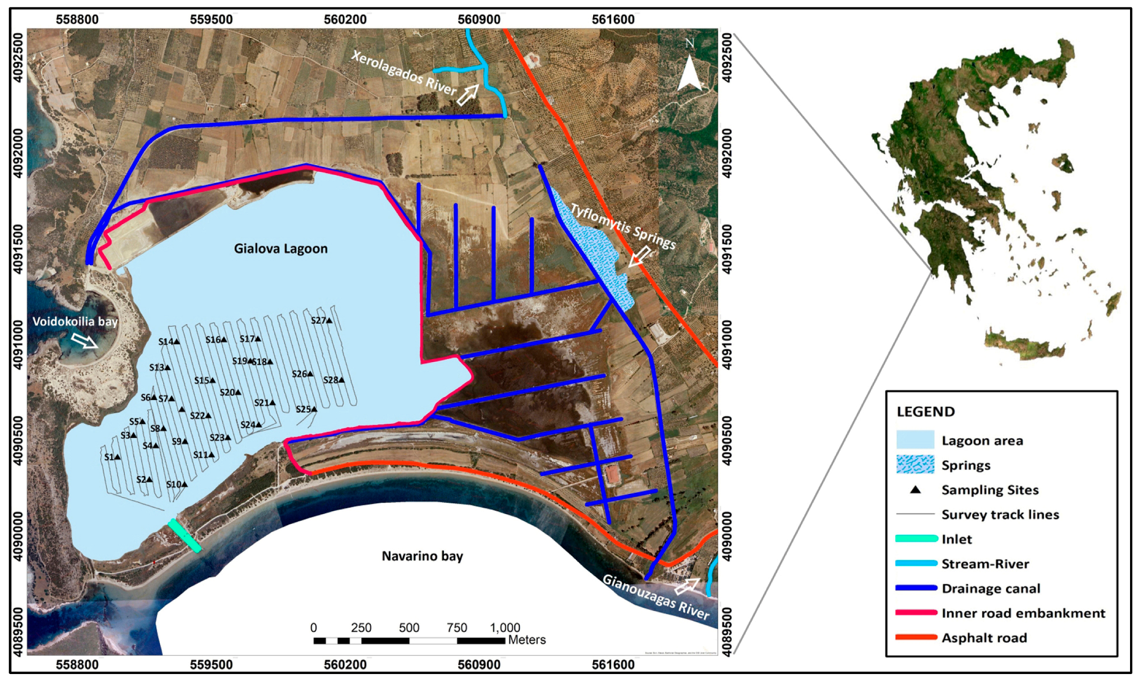
2.1. Study Area

The Gialova lagoon (Figure 1) is located in the SW Peloponnese, Greece, separated from the Navarino bay (Ionian Sea, Eastern Mediterranean) by a 3.3 km long and 0.15 km wide sand barrier. The interaction with the bay occurs through a narrow inlet that is formed on the barrier. The surrounding geological setting of the Gialova lagoon consists of Holocene alluvial deposits and dunes, Plio-Pleistocene conglomerates, marls, and sandstones, and Eocene to Oligocene turbidites, while the alpine bedrock consists of Upper Cretaceous to Eocene limestones [32]. Core sediment records from the Gialova lagoon and the surrounding wetland reveal that this coastal setting has been highly vulnerable and prone to climatic and environmental shifts over the last 5000 years, including subjection to extended dry or wet periods and exposure to high-energy tsunamigenic events [37,38,39].

The lagoon is fed in freshwater and sediment by the Xirolagkados River and Tyflomyti springs (Figure 1). Before the 1950s, the Xirolagkados River was the main sediment supplier discharging in the northern sector of the lagoon, while Tyflomyti springs occurred in the eastern margin, pouring freshwater into the lagoon and the adjoining marshes of the Gianouzagas River plain [31,32]. Nevertheless, during the 1950s, the Xirolagkados River and Tyflomyti springs were diverted to Voidokoilia Bay and Navarino Bay, respectively. Currently, groundwater from the neighboring alluvial plain, together with the construction of two canals that have restored the connection with the Xirolagkados River and Tyflomyti springs since 1998, allow the input of freshwater into the lagoon [35,36].

The lagoon is quite shallow, while the hydrological regime shows intense seasonal variations, affected by the equilibrium between evaporation and precipitation/freshwater input [40]. Water temperature and salinity range between 15–32 °C and 30–70‰, respectively, the pH values between 7 and 9 and the dissolved oxygen levels between 4 and 11 mg/L, with the latter being higher in the winter season [40,41]. Concerning trophic state levels, the lagoon is characterized as eutrophic in April and hypereutrophic in August regarding phosphate content, whereas ammonium concentrations exhibit high values on an annual basis [40]. The high trophic levels are in line with the extended seagrass growth in the lagoon, as over 25% of its bottom is covered by submerged aquatic vegetation [42]. Notably, during the summer season, the eastern part of the lagoon becomes partially dried out.

2.2. Fieldwork

A combined acoustic (bathymetric) and sampling survey was conducted in the autumn of 2020. Bathymetric data were obtained using a high-resolution sonar (Lowrance—Elite-5 Ti) equipped on board an unmanned surface vehicle (USV) [43]. The imprinting of the lagoon’s bathymetry was accomplished using a TotalScan-type sensor, while coverage was attained in the 20 m slant range, achieving 25% overlapping. Further, a 455 kHz operation pulse frequency was selected as the optimum choice due to the extremely shallow waters and high turbidity in the water column, most probably due to the presence of suspended solids (nutrients) and/or bottom sediment resuspension.

The design of track lines (Figure 1) was made on Mission Planner Software version 1.3.74, to support USV navigation on water. The USV platform was further equipped with a Global Positioning System (GPS—Magellan NAV 6500) for the positioning data and a high-resolution digital camcorder placed in a waterproof case for the data ground-truthing. For the position of USV during operation, real-time kinematic satellite navigation technology (RTK GPS) (Emlid Reach M2) was used, based onshore, with less than 10 cm accuracy. For the acquisition of the data, USV operated in water at 1 m/s speed (≈2 knots) for about nine working hours in total.

The sampling campaign was designed following the bathymetric survey. Twenty-eight (28) surficial sediment samples (Figure 1) were collected from pre-defined sampling sites, oriented by the backscatter data gained from the acoustic survey, covering the entire spectrum of the different backscatter levels. The samples were collected using a Van–Veen grab, corresponding to the upper ~20 cm of the lagoon’s bottom, while positioning was determined with a Garmin GPS 60 device. Sub-samples for laboratory analyses (S1–S28) were taken from the central part of the grab to avoid contamination, sealed in polyethylene bags, and stored at 4 °C until the beginning of laboratory analyses. Systematic sediment sampling is considered a very effective ground-truthing technique in the acoustic survey.

2.3. Laboratory Analyses

2.3.1. Sedimentology

The sedimentological examination of the 28 collected samples included macro- and microscopic textural and compositional observations, together with grain size analysis. Macroscopic description is aimed at the general characterization of the sample, focusing primarily on features such as color (based on the Munsell Color Chart), lithology, and abundance of biogenic material. Microscopic observations were performed in the sand fraction of the samples (grain size > 63 μm, or <4Φ, see below) using a Leica MZ6 binocular stereo microscope after wet sieving and drying the retained fraction.

Grain size analysis was carried out by laser diffraction using a Malvern Mastersizer 2000 particle analyzer. Hydrogen peroxide (H₂O₂) treatment was applied before analysis to eliminate organic matter. The logarithmic (original) graphical measures of Folk and Ward, [44] were calculated with the GRADISTAT software version 8.0 [45], while sediment classification followed the nomenclature of Folk [46]. Accordingly, the five statistical parameters: median (Md), mean size (Mz), sorting (σi), skewness (Sk), and kurtosis (KG) of the grain size distribution as well as the size fractions are expressed in the logarithmic phi scale (Φ). Thus, sand, silt, and clay regard the size fraction as between −1Φ–4Φ, 4Φ–8Φ, and >8Φ, respectively [46].

The interrelationships between grain size and statistical parameters were examined in order to investigate the prevailing environmental conditions during sediment deposition [12,46]. We used the bivariate diagram of median (Md) versus sorting (σi) to differentiate between riverine, wave, and quiet water processes in a lagoonal setting [47] and the most appropriate of the discriminant functions proposed by Sahu [48], which suggests a higher influence between shallow marine versus fluvial (deltaic) environments: Y_sm:f = 0.2852 × Md − 8.7604 × σi² − 4.8932 × Sk + 0.0482 × KG. When Y < −7.4190, a fluvial (deltaic) deposit is indicated, whereas when Y > −7.4190, shallow marine conditions prevail. The above proxies concern the statistical parameters obtained through the original graphical method of Folk and Ward [44] and have been widely used in the research of lagoonal and coastal settings [49,50,51,52].

2.3.2. Geochemistry

Bulk geochemistry and Total Organic Carbon (C_org) analyses in the 28 samples were both conducted at ALS Geochemistry Ltd. (Loughrea, Ireland), certified to ISO/IEC 17025:2017. Bulk geochemical analysis targets the elemental composition of the sediment. It was performed through a multi-element ultratrace method that combined four-acid digestion (HCl, HNO₃, HClO₄, and HF) with an inductively plasma—mass spectrometry (ICP—MS) finish. The four-acid digestion breaks down most silicate and oxide minerals, allowing for a “near-total” recovery of most analytes. The following forty-three (43) major and trace elements were determined: Al, Ca, Fe, K, Mg, Na, S, Ti (major, %) and Ag, As, Ba, Be, Cd, Ce, Co, Cr, Cs, Cu, Ga, Hf, In, La, Li, Mn, Mo, Nb, Ni, P, Pb, Rb, Sb, Sc, Sn, Sr, Ta, Th, Tl, U, V, W, Y, Zn, Zr (trace, ppm). Total organic carbon content (C_org) was determined using a LECO furnace carbon analyzer. Pre-treatment with HCl (25%) was necessary for removing inorganic carbonates.

2.3.3. Benthic Foraminifera

Benthic foraminifera tests were studied in 14 samples. Each sample was wet-sieved through 125 μm, then oven-dried at 50 °C. A number of 200–300 foraminiferal tests were used for microfaunal analysis. In cases where the dried residue exceeded the 200–300 tests of benthic foraminifera, it was split with a microsplitter in order to provide an adequate number. Then, each sample was weighed, and each foraminifera specimen was picked and identified up to the species level when possible based on the World Register of Marine Species database taxonomy (WoRMS). In addition, foraminiferal parameters have been calculated, like foraminiferal abundance (number of specimens per 1 g of dry sediment), relative foraminiferal abundance (the percent composition of a certain species relative to the total number of foraminifera), and Shannon-Weaver index ($Hs=-{\sum }_{i=1}^R{p}_{i}ln{p}_i$) as an estimation of the species diversity.

2.4. Contamination Assessement

For the assessment of the metal contamination levels and the possible anthropogenic impact on the sediments of Gialova lagoon, three (3) of the most commonly used pollution indices were employed: (a) Enrichment Factor (EF), (b) Geo-accumulation Index (I-geo), and (c) Pollution Loading Index (PLI) [17,26]. The global average shale values proposed by Turekian and Wedepohl [53] were used as natural background sediment reference concentrations. Additionally, for the implementation of the Foram-AMBI index, foraminiferal species were assigned to one of five ecological groups, according to the sensitivity of species to increasing stress [27,28,29]. The assignment of each species to an ecological category was mainly based on the list of species from intertidal and transitional waters in the Mediterranean Sea [29] and similar ecological areas that were found in the literature (e.g., [28]). All the above is summarized in

Table 1. Environmental Indices used in the present study.

Index	Procedures of Calculation	Values	Description-Classification	Reference
EF	EF = (Metal/RE)sample/(Metal/RE)background. “RE” stands for the Reference Element. Aluminum (Al) was selected as the most suitable reference element, as it is mostly indicative of the natural, lithogenic fraction of the sediments [54].	EF ≤ 1 1 < EF ≤ 3 3 < EF ≤ 5 5 < EF ≤ 10 10 < EF ≤ 25 25 < EF ≤ 50 EF > 50	No enrichment Minor enrichment Moderate enrichment Moderate to severe enrichment Severe enrichment Very severe enrichment Extremely severe enrichment	[55]
I-geo	I-geo = log2 (Cn/1.5Bn), where Cn is the measured content of element “n”, and Bn is the background content of the “n” element.	Igeo ≤ 0 0 < Igeo < 1 1 < Igeo < 2 2 < Igeo < 3 3 < Igeo < 4 4 < Igeo < 5 Igeo ≥ 5	Unpolluted Unpolluted to moderately polluted Moderately polluted Moderately to heavily polluted Heavily polluted Heavily to extremely polluted Extremely polluted	[56]
PLI	PLI = (CF1 × CF2 × CF3 × … × CFn)1/n where CFmetals is the ratio between the content of each metal to the background values in sediment; CFmetals = Cmetal/Cbackground. The PLI ascribes an evaluation of the overall toxicity status of the sediments.	PLI < 1 PLI = 1 PLI > 1	Unpolluted sediments Baseline level of contamination Progressive deterioration of the environmental conditions and increasing pollution	[57]
Foram-AMBI	AMBI = {(0*%GI) + (1.5*%GII) + (3*%GIII) + (4.5*%GIV) + (6*%GV)}/100 Where GI-GV the relative abundance of each ecological group. Specifically, GI is the “sensitive species”, GII “Indifferent species”, GIII “3rd-order opportunistic species”, GIV “2nd-order opportunistic species” and GV “1st-order opportunistic species”	0 < AMBI ≤ 1.2 1.2 < AMBI ≤ 3.3 3.3 < AMBI ≤ 4.3 4.3 < AMBI ≤ 5.5 5.5 < AMBI ≤ 7	High Ecological Quality Status (EcoQs) Good EcoQs Moderate EcoQs Poor EcoQs Bad EcoQs	[28,58]

, including basic information for each index.

2.5. Statistical Treatment—Hierarchical Clustering and Factor Analysis

Hierarchical clustering was performed on the grain size distribution (GSD) data using the statistical software SPSS v27 to identify possible similarities between the GSD curves and, consequently, classify the samples into distinct groups. Clustering was based on Ward’s method with Squared Euclidean distance intervals.

Factor analysis is a multivariate statistical method that detects any interrelationships within a set of variables (R-mode) or objects (Q-mode) [59]. Factor analysis has been successfully used in the sedimentary research of Greek lagoons, unraveling certain patterns in the distribution of heavy metals, organic material, and textural components [16,20,60]. R-mode factor analysis was performed to investigate the interrelationships between the examined geochemical parameters (variables) and identify the processes that explain their spatial distribution as well as possible common sources [61,62], whereas Q-mode factor analysis was designed to investigate interrelationships between samples (objects) on the basis of geochemical properties (variables).

The aims of the Q-mode analysis, according to Reyment and Joreskog [59], are: (i) to find the minimum number of “end-members” needed to account for the compositional variation observed (ii) to identify the composition of the “end-member” in relation to the original variables; and (iii) to describe each sample in terms of the “end-member”. To bring to fruition the aims of the Q-mode analysis, a plot of factor loadings for the first two factors was constructed, the loadings of which were normalized by being divided by their communalities.

In the current study, R-mode and Q-mode factor analysis were conducted via the statistical software program IBM SPSS v27 on the whole geochemical dataset, containing 28 samples × 44 variables (C_org and the 43 major and trace elements; see Supplementary File S3). The analysis was conducted following the steps described by Papatheodorou et al. [63].

3. Results and Discussion

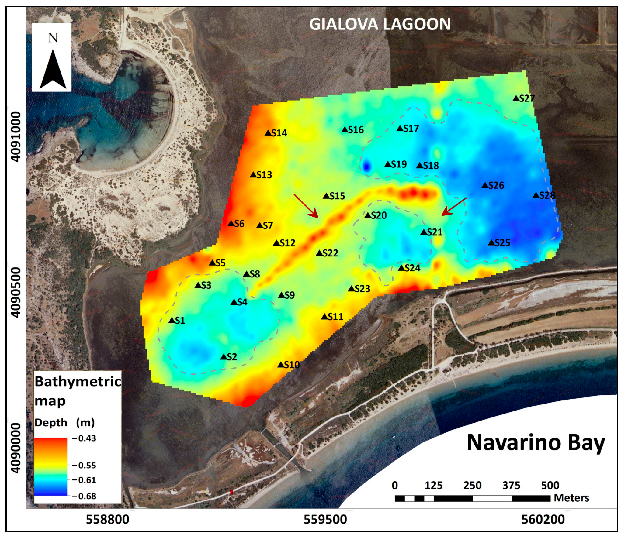
3.1. Bathymetry

The acquired acoustic data showed that Gialova Lagoon is very shallow, with water depths up to 0.7 m. The detailed bathymetry showed that the lagoon floor is not flat, but the variation in topography forms three small-sized basins located in the eastern, central, and western parts of the examined area (Figure 2). The highest depths occur in the eastern part, while in the western basin, two smaller sub-basins are distinguished. The shallower depths were obtained along the borders and in the central part of the lagoon. Yet, it is worth mentioning the clear view of an elongated ridge running from east to southwest at the central part of the lagoon, which could possibly be related to fishing activities [30,33] (Figure 2). Moreover, traces of another ridge have been observed running the lagoon from north to south.

3.2. Sedimentology

3.2.1. Grain Size Distribution

The grain size analyses of the collected bottom sediment samples (Supplementary File S1) showed that the average proportion of sand, silt, and clay is in the order of 7.50%, 63.17%, and 29.32%, respectively, while the mean size (Mz) ranged from 4.99 Φ to 7.28 Φ, with an average value of 6.67 Φ, implying that the lagoon’s sediments are composed principally of silt-sized sediments.

The coarser sediments accumulate along the southwestern border of the lagoon, just north of the sandy barrier that separates the lagoon from Navarino Bay (Figure 3a). However, the distribution of the fine material does not exactly follow the morphology of the lagoon’s floor. The high percentage of clay and the high values (Φ) of Mz (Figure 3b,c) are not located in the three shallow basins of the lagoon but slightly north of them.

The Gialova sediments are characterized as poorly to very poorly sorted, with σi values ranging from 1.25 Φ to 3.03 Φ, with an average value of 1.80 Φ (Figure 3d). Sorting values follow the trend of sand content, presenting the highest values along the southwestern border of the lagoon and diminishing towards the central part. Skewness (Sk) displays low variability and ranges between −0.36 Φ and 0.02 Φ with an average value of −0.17 Φ (Supplementary File S1), thus characterizing mainly coarse-skewed sediments. Finally, kurtosis fluctuates between platykurtic and mesokurtic values (KG: 0.68–1.06 Φ), with an average value of 0.91 Φ (Supplementary File S1).

3.2.2. Sand Composition

The microscopic examination led to the determination of three major classes that comprise the sand grains: (a) lithological components (detrital lithics and various mineral grains)—(b) biogenic components (fragments and/or individual specimens of benthic foraminifera, gastropods, ostracods, bivalves, etc.)—(c) organic components (wood fragments, algal constituents, and pyritized features). The relative proportions of lithogenic, biogenic, and organic components in the sandy material were determined on a semi-quantitative basis, as described by Chevillon [11]. The mean proportions of the above classes are 33%, 62%, and 5% for the lithogenic, biogenic, and organic grains, respectively (Supplementary File S1), suggesting that the sandy material of Gialova sediments is primarily of biogenic origin.

3.2.3. Insights on the Depositional Environment

The overall sedimentological work indicates a number of common features among the studied samples, which, in turn, reflect similar processes at the sampling sites. At first, all samples are fine-grained (dominant mud and silt) and accompanied by various seagrass residues and skeletal remains (Supplementary File S2, Table S1), thus suggesting a low-energy environment and adequate biogenic productivity. The sand content throughout the lagoon has a principally bioclastic composition (as mentioned in the previous section), comprising fragments and individuals of mollusk shells (gastropods and bivalves), ostracods, and benthic foraminifera. Bioclastic sand is commonly observed in lagoons and is closely related to increased organic productivity and seagrass growth [11,64,65,66]. The prevalent low-energy conditions are further supported by the bivariate Md—σi plot on the grain size data, while the discriminant function analysis indicates that the fluvial influence overcomes the effects of seawater intrusions throughout the lagoon [47,48] (Supplementary File S2, Figure S2).

Secondly, all samples share the same very dark gray color according to the Munsell Color Chart (5Y 3/1) implying similar eutrophic conditions throughout the lagoon [1]. This is further supported by the relatively high and weakly varying C_org values of the samples (1.35–2.02% range, mean value: 1.67%;

Table 2. Mean, minimum, and maximum values of the major and trace elements and organic carbon (C_org) in the surface sediments of Gialova lagoon.

Element	Unit	Mean	Min	Max
Ag	ppm	0.03	0.02	0.05
Al	%	4.47	3.11	5.33
As	ppm	8.40	6.20	10.00
Ba	ppm	136.79	110.00	160.00
Be	ppm	1.22	0.87	1.50
Ca	%	11.18	7.48	16.05
Cd	ppm	0.13	0.10	0.16
Ce	ppm	37.99	35.40	40.80
Co	ppm	14.81	10.30	17.40
Cr	ppm	122.50	91.00	151.00
Cs	ppm	4.06	2.70	4.93
Cu	ppm	30.50	20.50	36.50
Fe	%	3.20	2.13	3.84
Ga	ppm	10.61	7.14	12.65
Hf	ppm	1.33	1.00	1.60
In	ppm	0.04	0.03	0.05
K	%	1.40	1.00	1.63
La	ppm	20.09	18.00	22.90
Li	ppm	43.01	31.20	50.20
Mg	%	1.97	1.27	2.25
Mn	ppm	1026.32	646.00	1150.00
Mo	ppm	6.32	3.26	8.90
Na	%	2.72	1.82	3.61
Nb	ppm	7.46	5.10	8.80
Ni	ppm	103.20	66.50	123.50
P	ppm	395.71	330.00	450.00
Pb	ppm	35.46	26.30	44.40
Rb	ppm	80.07	55.20	95.20
S	%	1.50	0.99	1.84
Sb	ppm	0.49	0.36	0.57
Sc	ppm	10.60	7.00	12.70
Sn	ppm	1.62	1.10	2.00
Sr	ppm	713.00	434.00	1145.00
Ta	ppm	0.48	0.33	0.57
Th	ppm	5.91	4.54	7.55
Ti	%	0.22	0.16	0.26
Tl	ppm	0.42	0.31	0.51
U	ppm	2.94	2.10	3.90
V	ppm	69.18	46.00	83.00
W	ppm	0.85	0.60	1.00
Y	ppm	16.97	13.50	18.70
Zn	ppm	64.50	45.00	79.00
Zr	ppm	48.38	32.70	59.80
Corg	%	1.67	1.35	2.02

) and agrees with the eutrophic character of the lagoon waters [40]. Thirdly, the large majority of the samples are characterized by coarse—skewed grain size distribution curves, likely reflecting a winnowing process along the lagoon bottom. This is a typical process in shallow lagoon environments and corresponds to the removal of the fine-grained distribution tail through re-suspension, induced by wind action [21,67,68].

However, and despite the above-mentioned similarities, the detailed examination through hierarchical clustering of the grain size distribution (GSD) curves plus the textural and compositional evaluation of the samples revealed the presence of four (4) dominant sedimentary facies that describe the lagoon’s bottom (Supplementary File S2, Figure S1, Table S1). These facies reflect the hydrodynamic variations within the lagoon, revealing different conditions between the western and eastern small basins (Facies 1 versus Facies 4) and the presence of a N-S-SW mixing zone (Facies 2 and 3). The four facies are thoroughly presented in Supplementary File S2.

3.3. Geochemistry

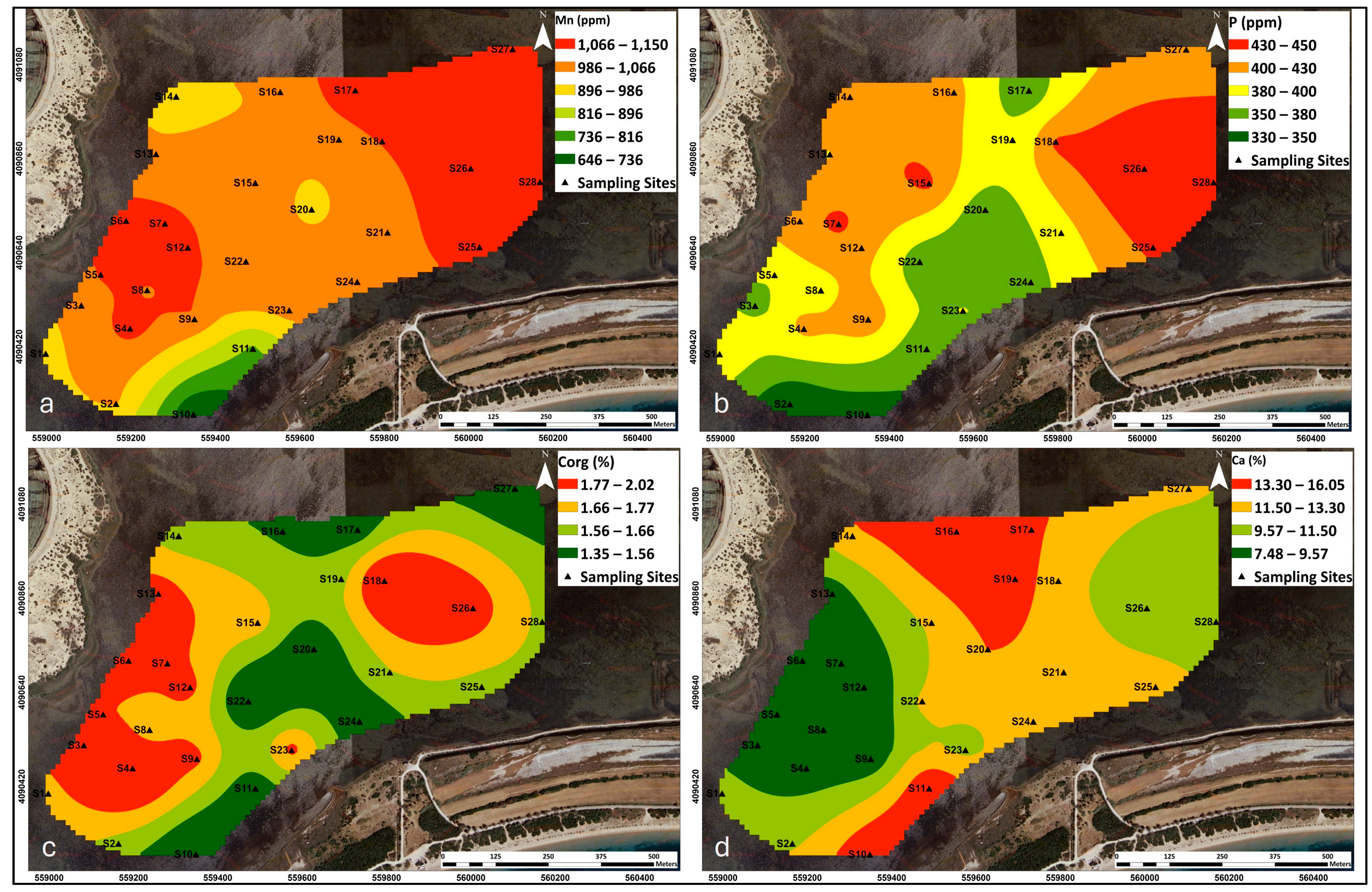
3.3.1. Elemental Concentrations in Gialova Lagoon Sediments

The concentration values of all measured major and trace elements, as well as organic carbon (C_org), are shown in Table 2. Additionally, the measured values per sample are presented in Supplementary File S3.

Herein, the spatial distribution of selected elements’ concentrations (Al, As, Ca, Cd, Cr, Cu, Fe, Mn, Mo, Ni, Pb, P, S, Zn) and C_org is discussed. Among them, specific elements have been grouped and described together due to their highly similar spatial distribution. These groups are Al-Cr-Cu-Fe-Ni-Pb-S-Zn (Group A) and As-Cd-Mo (Group B). The distribution of the other elements (Ca, Mn, P, and C_org) is discussed separately.

The maximum concentrations of Group A elements are observed slightly north of the western shallow basin (Figure 4). Low concentrations are detected at the southwestern margin, close to the communication channel (inlet) with Navarino Bay, and at the northern part of the lagoon.

The spatial distribution pattern of Group B metals shows two areas of maximum concentrations: (i) at the western sub-basin of the shallow western basin and (ii) at the shallow area between the western and eastern basins of the lagoon (Figure 5). Low concentrations are measured at the eastern and northern margins of the lagoon and close to the inlet.

Manganese (Mn) shows a different spatial pattern compared to those of Groups A and B. The maximum concentrations are found at the eastern shallow basin and at the north of the western shallow basin (Figure 6a). Furthermore, low Mn concentrations are measured close to the inlet (Figure 6a).

The concentration of phosphorus (P) shows the highest values at the eastern shallow basin of the lagoon, while it is also increased along the northwestern sector (Figure 6b). On the other hand, low values are observed near the inlet and across a zone that extends from the southern part towards the central and northern sides of the lagoon.

The C_org values vary between 1.35 and 2.02% with a mean content of 1.67%, which is a typical range for Mediterranean coastal lagoon sediments [14,21,23,69]. The spatial distribution of C_org is shown in Figure 6c. The highest C_org percentages (>1.8%) were measured at the eastern sub-basin of the shallow western basin and at the western part of the eastern shallow basin, while low concentration values (<1.5%) were obtained along the sand-rich depositional zone behind the barrier as well as the central part and northern margin of the lagoon. This pattern highlights the enhanced adsorption of organic matter in the fine silt and clay fractions of the sediment. It also suggests that organic matter is primarily deposited in the two depressed morphological basins where the burial process prevents oxidation and that the oxygenation of the lagoon is ascribed to the saline water inflows from the adjacent Navarino Bay through the inlet.

Calcium (Ca) concentration in Gialova lagoon sediments is found between 7.48 and 16.05% (mean value: 11.18%) and shows an almost opposite distribution pattern with Group A elements (Figure 4 and Figure 6d). Specifically, the maximum concentrations (>13%) are noticed in the northern sector and close to the inlet, whereas the minimum values (<9.5%) lie in the western shallow basin.

3.3.2. Geochemical Comparison with Other Greek Lagoons

The range of Cd, Cr, Cu, Fe, Mn, Ni, Pb, V, and Zn concentrations found in the present study are comparable with those from other lagoonal and coastal environments in Greece (

Table 3. Mean values of selected heavy metal concentrations in the Gialova lagoon compared to other Greek aquatic systems and average Shales’ proportion.

Element	Cd	Cr	Cu	Fe	Mn	Ni	Pb	V	Zn	Reference
Element Unit	ppm	ppm	ppm	%	ppm	ppm	ppm	ppm	ppm
Gialova lagoon	0.13	122.50	30.50	3.20	1026.32	103.20	35.46	69.18	64.50	This study
Gialova lagoon	0.81	118.20	57.51	4.76	1549	172.11	36.29	69.24	98.47	[32]
Messolonghi Lagoon	–	101.00	20.00	2.36	630.00	84.00	16.00	75.00	60.00	[16]
Koumoundourou Lake	–	58.00	21.00	0.58	155.00	28.00	53.00	23.00	83.00	[70]
Alikes Lagoon	–	251.67	29.17	3.59	630.00	134.17	9.88	109.33	68.89	[71]
Aetoliko Lagoon	–	140	88	4.17	837	75.6	–	–	122.2	[72]
Kleisova Lagoon	–	–	13.00	1.64	562.00	62.00	–	–	29.00	[60]
Rhodia Lagoon	–	231	37	2.83	867	124	36	112	72	[73]
Tsoukalio Lagoon	–	274	31	3.16	1191	131	26	108	76	[73]
Logarou Lagoon	–	302	44	4.74	922	221	25	153	105	[73]
Tsopeli Lagoon	–	295	48	3.98	665	168	26	129	100	[73]
Navarino Bay—upper sediments	–	–	66.00	–	–	151.00	–	–	352.00	[74]
Mean		196.76	38.87	3.18	800.8	119.99	28.52	97.32	81.45
(min-max)		(58–302)	(13–88)	(0.58–4.76)	(155–1549)	(28–221)	(16–36.3)	(23–109.3)	(29–122.2)
Average Shales	0.3	90	45	4.72	850	68	20	130	95	[53]

) and are usually lower than the mean concentration for those elements. Exceptions are Mn and Pb, which present higher concentrations in Gialova lagoon (present study) in relation to their mean concentrations found in other lagoonal and coastal environments in Greece. In addition, the comparison of the mean concentrations of Cd, Cr, Cu, Fe, Ni, V, and Zn found in the present study is lower than the average shale values, but that of Mn and Pb is higher.

Moreover, when comparing the metal concentration values in Gialova sediments between 2020 (this study) and 1995 [32], there is an evident downslope trend for several metals, such as Cd, Cu, Mn, Ni, and Zn. This decline in metal concentrations could be partially attributed to the different analytical methods employed in the two studies; however, it could also indicate efficient modifications in the recent environmental conditions and/or changes in sedimentary processes (see Section 3.7).

3.4. Benthic Foraminifera

A total of 26 benthic foraminiferal species were identified in the samples. These are Ammonia spp., Ammonia parkinsoniana, Ammonia perlucida, Ammonia tepida, Asterigerinata mammila, Bulimina marginata, Cassidulina sp., Cibicides spp., Elphidium crispum, Elphidium sp., Eponides sp., Gyroidina sp., Haynesina germanica, Lenticulina orbicularis, Melonis baleaanus, Miliolinella subrotunda, Nonion spp., Quinqueloculina auberiana, Quinqueloculina seminula, Quinqueloculina vulgaris, Quinqueloculina spp., Rosalina globularis, Spiroloculina sp., Triloculina trigonula, Rectuvigerina phlegeri, and Valvulineria sp.

The relative abundance of recognized species varies from site to site, while only nine species show relative abundances greater than 2% in at least one sample (Supplementary File S4). The foraminifera microfauna is largely dominated by A. tepida (73.75% on average), followed by A. parkinsoniana (15.12% on average), and Q. seminula (3.23% on average). The foraminifera abundance varies from 510.7 indv/g in S13 to 5225.9 indv/g in S15, with an average value of 1492.5 indv/g. The Shannon–Weaver index (Hs) ranged from 0.65 (S28) to 1.25 (S13), with an average value of 0.85.

In addition, morphological abnormalities have been observed in most sampling sites, except for S13 and S28, while the highest abundance of deformed individuals was observed at S18 (6.6% of total fauna). The deformed assemblage is exclusively the species Ammonia tepida, which is 3.31% on average in the total fauna and 4.7% of the Ammonia tepida fauna. The abnormalities in hyaline specimens are likely associated with imperfect biomineralization [75] that can be attributed to the development of cavities in the wall or to disorganization in the pattern of crystallites [76]. Environmental factors such as pollution and/or environmental stress are potential factors that could contribute to the observed disorganization [76].

3.5. Geochemical Processes—Elemental Source Identification

The results of the R-mode factor analysis analysis led to the discrimination of certain geochemical processes along the bottom sediments and allowed the identification of possible sources from which the metals have been derived into the lagoon.

A four (4) factor model was utilized to describe the geochemical dataset without losing significant information. These factors explain about 92% of the total variance, and each variable shows communalities higher than 0.65 (

Table 4. Communalities and varimax rotated R-mode factor loadings (R-mode) of the geochemical dataset. Variables with loadings ≥0.4 are highlighted in bold. High negative loadings are indicated in italics.

Variable	Communalities	Rotated Component Matrix
		Factor 1	Factor 2	Factor 3	Factor 4
Ag	0.646	0.731	0.299	−0.141	0.046
Al	0.995	0.927	0.257	0.253	0.074
As	0.796	0.242	0.736	0.374	−0.236
Ba	0.947	0.901	0.249	0.268	0.028
Be	0.977	0.943	0.218	0.197	0.044
Ca	0.928	−0.898	−0.106	−0.191	−0.272
Cd	0.789	0.650	0.605	0.027	−0.010
Ce	0.856	0.494	−0.102	0.304	−0.713
Co	0.971	0.862	0.359	0.311	0.039
Cr	0.876	0.929	−0.038	−0.029	−0.101
Cs	0.993	0.917	0.294	0.248	0.058
Cu	0.982	0.899	0.292	0.274	0.110
Fe	0.995	0.903	0.264	0.319	0.095
Ga	0.994	0.913	0.275	0.273	0.102
Hf	0.918	0.904	0.231	0.210	0.060
In	0.906	0.790	0.339	0.362	0.186
K	0.990	0.897	0.280	0.277	0.177
La	0.881	0.556	0.162	0.544	−0.500
Li	0.935	0.860	0.380	0.221	0.048
Mg	0.958	0.677	0.186	0.432	0.527
Mn	0.911	0.297	0.144	0.800	0.403
Mo	0.926	0.369	0.884	0.036	−0.086
Na	0.757	0.265	−0.016	0.191	0.806
Nb	0.989	0.902	0.254	0.313	0.113
Ni	0.993	0.894	0.334	0.279	0.061
P	0.829	0.183	−0.169	0.212	0.850
Pb	0.973	0.927	0.239	0.236	−0.014
Rb	0.994	0.910	0.304	0.260	0.072
S	0.919	0.780	0.403	0.386	0.003
Sb	0.868	0.126	0.883	0.171	0.209
Sc	0.992	0.914	0.285	0.260	0.086
Sn	0.974	0.928	0.188	0.237	0.146
Sr	0.904	−0.908	−0.064	−0.246	−0.123
Ta	0.976	0.911	0.239	0.288	0.075
Th	0.897	0.849	0.105	0.406	0.006
Ti	0.996	0.924	0.254	0.264	0.090
Tl	0.972	0.938	0.267	0.129	0.059
U	0.830	0.387	0.824	−0.007	−0.027
V	0.975	0.890	0.361	0.219	0.067
W	0.945	0.889	0.204	0.322	0.093
Y	0.934	0.485	0.169	0.813	0.098
Zn	0.986	0.925	0.308	0.187	0.041
Zr	0.854	0.733	0.217	0.519	0.015
Corg	0.702	0.597	0.295	−0.033	0.508
Explained Variance (%)		61.506	12.784	10.215	7.378

). This means that the four-factor model expresses the analyzed variables efficiently [59].

Factor 1 explains the largest proportion (61.5%) of the total variance and can be considered a bipolar factor (Table 4). It displays high positive loadings for Al, Ba, Be, Co, Cr, Cs, Cu, Fe, Ga, Hf, In, K, Li, Nb, Ni, Pb, Rb, S, Sc, Sn, Ta, Th, Ti, Tl, V, W, and Zn and moderate positive loadings for Ag, Cd, Ce, La, Mg, Y, Zr, and C_org. In contrast, Ca and Sr show high negative loadings, constituting the negative pole of the factor.

Based on the loadings of the positive pole of Factor 1, this pole can be identified as the “terrigenous aluminosilicates” factor pole and represents the terrigenous inputs with a rather constant mineralogical sediment composition. Al, Fe, K, and Ti are major constituents of common silicate minerals and originate from the weathering release of parent materials in the local bedrock [77,78]. Additionally, Mg, Ni, Nb, and Rb provide good geochemical proxies for clay minerals, such as kaolinite, chlorite, illite, and smectite [79,80].

The terrigenous aluminosilicates factor pole exhibits a close relationship with C_org, as indicated by the moderate positive factor loading (Table 4). Several previous studies in shallow coastal areas and lagoonal environments have shown that clay minerals and organic matter build aggregates and flocs that absorb trace metals and then sink to form a “fluffy layer” [81,82]. Although the “fluffy layer” was not observed and sampled during the Gialova survey, its existence cannot be excluded. Moreover, the low-moderate (0.39) loading of U on Factor 1 could be related to the adsorption and complexion of U in humic organic material and poorly crystalline clay minerals [83,84]. It is also important to mention that although most of the elements with high positive loadings on Factor 1 are mostly of terrigenous origin, some of them could also be absorbed onto the aluminosilicate/C_org particles from anthropogenic sources. Based on the above, the positive pole of Factor 1 can be considered a “terrigenous aluminosilicate associated with C_org” factor, which additionally represents the potential adsorption of trace metals.

The high factor loading of S (0.780) combined with Fe (0.903) and many other heavy metals may outline acid-volatile sulfides (AVSs), a geochemical phase that contributes to the binding of metals [85]. AVS is an operationally defined reactive sulfide fraction that mainly comprises dissolved (hydrogen) sulfides and mackinawite (FeS), which may differ largely in their composition and capacity for precipitating trace metals in different aquatic environments [85]. It should also be mentioned that the existence of more stable forms of sulfides, like elemental sulfur and pyrite (FeS₂), cannot be excluded for Gialova lagoon. Consequently, the contribution of sulfur in the first factor further supports that a portion of metals could be absorbed by C_org and sulfides and do not hold solely lattice-held positions in the aluminosilicate minerals.

The high negative loadings of Ca and Sr in this factor imply an antipathetic relationship between the autochthonous biogenic carbonates and the terrigenous aluminosilicates. The element assemblages of Ca and Sr behave similarly to each other due to their similar ionic radius (rSr = 0.113 nm vs. rCa = 0.099 nm) and are the dominant components of most bioclastic materials in sediments [77,86]. In the present study, Ca presents a strong correlation with Sr and, contrariwise, a high anti-correlation with all typical terrigenous elements (Al, Ti, K, Fe, Rb, etc.). Notably, the macro- and microscopic examination of sediments suggests that the calcium carbonate component is principally of biogenic origin in Gialova lagoon, thus indicating that the primary production rates overcome the detrital intrusions of the distant limestone bedrock. Hence, the Ca and Sr loadings comprise the negative pole of Factor 1, associated with biogenic sedimentation.

Overall, the inverse relation between the main element assemblages of Factor 1 is the dominant geochemical process of the surface sediments of Gialova Lagoon, as indicated by the very high variance explained by the analysis. A similar “terrigenous aluminosilicates vs. autochthonous biogenic carbonates” bipolar factor was also determined in the geochemical data of other lagoons in western Greece (Messolonghi lagoon, [16]; Prokopos lagoon, [20]), thus highlighting the competitive contrast between detrital and biogenic sedimentation in lagoonal environments of the wider region.

The positive pole of Factor 1 (terrigenous aluminosilicates) shows high score values at the two basins of the lagoon and in the area north of the western one (Figure 7a). This pattern follows the distribution of clay and sediment mean size (Mz) (Figure 3b,c), which further indicates the potential adsorption of trace metals and C_org into the finer-grained fractions of the sediments [21,87]. The increased metal and C_org loads at the two basins hint at increased eutrophication levels and seagrass growth [88,89] but are not related to significant CaCO₃ deposition.

Regarding the negative pole of Factor 1 (autochthonous biogenic carbonates), it shows high values at the southern, central, and especially northern parts of the Gialova lagoon, forming a N-S-SW distribution zone (Figure 7a). At these parts of the lagoon, sediments of Facies 2 and 3 prevail, characterized by increased sand (mostly biogenic) and the common presence of seagrass residues (Supplementary File S2, Figure S1). These sediments display mainly platykurtic and bimodal grain size distributions, which could be explained by one of the following: (a) an elevated proportion of the coarser-grained fractions; (b) mixing processes; or (c) both.

The second factor (Factor 2) accounts for 12.8% of the total variance of the variables (Table 4) and shows high positive loadings on Mo, Sb, and U and moderate positive loadings on As, Cd and S.

The loading profile and the moderately positive loading of S suggest that this factor can be considered a solely “sulfide” factor. Mo, As, and Sb show intense correlation against S, as indicated by the high to moderate loadings, representing an anoxic phase in the surface sediments of the lagoon [24,90]. Divalent metals, such as Cd, have a high affinity with sulfides in sediments, especially in anoxic conditions [91]. Sulfides act as good scavengers of divalent metals that are trapped in the solid phase. Redox-sensitive metals like Mo and U show a similar distribution pattern, suggesting that redox processes are responsible for the deposition of both of these elements in the lagoon [90,92]. Moreover, Mo may be related to algal blooms because this element is essential for cyanobacterial uptake of nitrogen [93,94]. It is thought that algal remnants with increased concentrations of Mo are transported to the seafloor attached to particulate matter.

The spatial distribution of Factor 2 scores (Figure 7b) shows that the influence of sulfides takes place in a wider area at the central part of the lagoon. Maximum values of Factor 2 scores are observed at the western sub-basin of the western shallow basin and at the western part of the eastern shallow basin, indicating the enhanced influence of sulfides to those areas.

Factor 3 accounts for 10.2% of the total variance and shows high positive loadings on Mn and Y while having moderate loadings on La, Zr, Mg, and Th (Table 4). Manganese (Mn) is one of the main geochemical phases in the lagoon sediments and an important scavenger of heavy metals. Based on the loading profile, Factor 3 can be considered a “Mn-hydroxide” factor. The factor loading of C_org is negligible, indicating the competition between C_org and Mn-hydroxides for scavenging heavy metals.

The high to moderate loadings of Y, La, Zr, Mg, and Th on Factor 3 probably represent the adsorption and/or co-precipitation of these five elements into amorphous Mn oxyhydroxides. The Yttrium (Y), Lanthanum (La), and generally the Rare Earth Elements (REEs) distribution in surface aquatic sediments is mainly controlled by scavenging processes, in particular by Mn–oxides [95,96]. Y, La, Zr, Mg, and Th also show moderate—to—high loadings on Factor 1 (terrigenous aluminosilicates), which suggests the terrigenous (lattice-held) fraction of those elements and/or the limited scavenging from the aluminosilicates [96].

The spatial pattern of the Factor 3 scores implies that the influence of the Mn-oxyhydroxides is more intense at the eastern shallow basin and in the area between the two shallow basins of the lagoon (Figure 7c).

Factor 4 is a bipolar factor and accounts for 7.4% of the total variance of the data. It exhibits high positive loadings on P and Na and moderate positive loadings on Mg, Mn, and C_org (Table 4). The negative pole of the third factor presents moderate negative loadings on Ce and La (Table 4).

Phosphorus (P) has a key role in aquatic environments and is considered not only as a primary nutrient for aquatic ecology but also as the most critical limiting nutrient for aquatic productivity [97]. Sedimentary total phosphorus (TP) can be obtained in fractions, namely inorganic-P (IP), organic-P (OP), P bound to Al, Fe, and Mn-oxyhydroxides (Mn-P), and calcium-bound P (Ca-P) [98]. In the case of the Gialova lagoon, the positive correlation of P to Na, Mn and C_org suggests at least three P-fractions in the lagoon sediments: (a) inorganic-P in the form of sodium polyphosphate compounds [99], (b) Mn-oxyhydroxides, and (c) organic-P (OP). Based on the above, the positive pole of the fourth factor can be considered a “phosphate” factor of both natural (OP, Mn-P) and anthropogenic (phosphate and polyphosphate fertilizers) origin.

Mg, as mentioned before, also shows a high positive loading on Factor 1, suggesting that Mg concentrations in the lagoon are controlled by multiple processes, such as the “terrigenous aluminosilicates” distribution (Factor 1) and the sea salt influence and/or chlorophyll a degradation (Factor 4). Magnesium, being the metallic part of chlorophyll, can be found in association with phytoplankton and macrophytic debris, which contribute to the organic matter content of the sediments. The Mg released through chlorophyll degradation during cellular senescence and death [100] could replenish some of the Mg content of the sediments [16]. The moderately positive loading of the C_org further suggests this interpretation. Moreover, Mg has been used in magnesium-fortified phosphate fertilizers [101], and as such, an additional, anthropogenic source is possible.

The high loadings of Ce and La on the negative pole of Factor 4 probably represent the “dissolved” form, which includes both truly dissolved and/or colloidal and/or the labile (hydroxylamine) form [102].

The “phosphates” factor pole has an important contribution at the northwestern and eastern parts of the lagoon, as indicated by the spatial distribution of the factor scores (Figure 7d). The northwestern part is directly affected by the Xirolagkados River mouth and discharges, so it is most probable that the high Factor 4 scores at this area indicate increased accumulation of materials related to phosphate fertilizers rather than organic-P compounds (low C_org values at the northwestern part; Figure 6c). On the other hand, the co-variation with the Factor 3 scores at the eastern basin suggests a predominant coupling of P to Mn-oxyhydroxides (Mn-P).

3.6. Contamination Assessment (Environmental Indices)

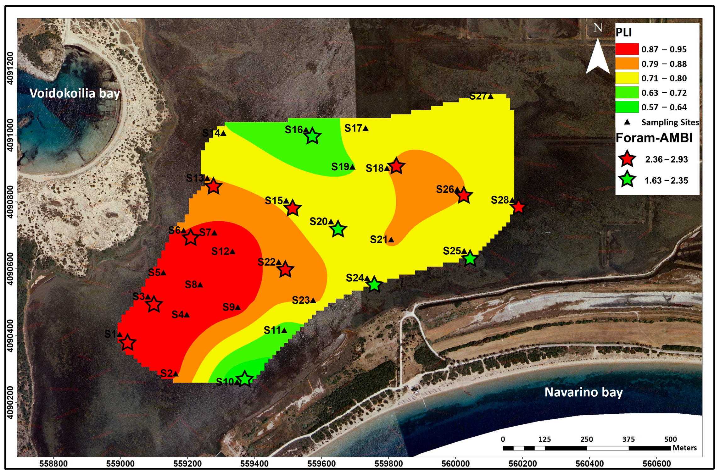
3.6.1. Heavy Metal Pollution Indices (EF, I-geo, PLI)

The application of the metal-related pollution indices regarded a total of 14 metals (Ag, As, Cd, Co, Cr, Cu, Mn, Mo, Ni, Pb, Sn, U, V, and Zn), which are typically used for contamination assessment in environmental studies due to their increased toxicity levels and hazardous impact on ecosystems and human health [103,104,105]. Concerning Enrichment Factor (EF) and I-geo indices, the results are presented and discussed in terms of the average values of the above metals in the lagoon sediments. The total results per sample are presented in Supplementary File S5 for both indices.

Based on the EF variation, the Gialova lagoon sediments are characterized by relatively low metal pollution levels (

Table 5. Contamination assessment of the Gialova lagoon sediments based on the Enrichment Factor (EF) and Geoaccumulation Index (I-geo) values for the pollution-indicator metals concentration.

	Enrichment Factor (EF)					Geoaccumulation Index (I-geo)
Metal	Min	Max	Mean	Class	State	Min	Max	Mean	Class	State
Sn	0.45	0.52	0.48	EF ≤ 1	No enrichment	−3.03	−2.17	−2.49	I-geo ≤ 0	Unpolluted
Cd	0.64	0.87	0.76	EF ≤ 1	No enrichment	−2.17	−1.49	−1.84	I-geo ≤ 0	Unpolluted
Ag	0.55	1.13	0.86	EF ≤ 1	No enrichment	−2.39	−1.07	−1.68	I-geo ≤ 0	Unpolluted
V	0.87	1.00	0.95	EF ≤ 1	No enrichment	−2.08	−1.23	−1.51	I-geo ≤ 0	Unpolluted
As	0.93	1.48	1.17	1 < EF ≤ 3	Minor enrichment	−1.65	−0.96	−1.23	I-geo ≤ 0	Unpolluted
Cu	1.15	1.25	1.21	1 < EF ≤ 3	Minor enrichment	−1.72	−0.89	−1.16	I-geo ≤ 0	Unpolluted
Zn	1.17	1.28	1.21	1 < EF ≤ 3	Minor enrichment	−1.66	−0.85	−1.16	I-geo ≤ 0	Unpolluted
Co	1.32	1.47	1.40	1 < EF ≤ 3	Minor enrichment	−1.47	−0.71	−0.95	I-geo ≤ 0	Unpolluted
U	1.03	1.69	1.43	1 < EF ≤ 3	Minor enrichment	−1.40	−0.51	−0.93	I-geo ≤ 0	Unpolluted
Mn	1.77	2.69	2.18	1 < EF ≤ 3	Minor enrichment	−0.98	−0.15	−0.32	I-geo ≤ 0	Unpolluted
Cr	2.13	3.43	2.45	1 < EF ≤ 3	Minor enrichment	−0.57	0.16	−0.15	I-geo ≤ 0	Unpolluted
Ni	2.52	2.79	2.71	1 < EF ≤ 3	Minor enrichment	−0.62	0.28	0.00	I-geo ≤ 0	Unpolluted
Pb	3.03	3.38	3.17	3 < EF ≤ 5	Moderate enrichment	−0.19	0.57	0.23	0 < Igeo < 1	Unpolluted to moderately polluted
Mo	2.18	5.49	4.36	3 < EF ≤ 5	Moderate enrichment	−0.26	1.19	0.66	0 < Igeo < 1	Unpolluted to moderately polluted

). More particularly, the sediments present no enrichment (EF ≤ 1) in four metals (Ag, Cd, Sn, V), minor enrichment (1 < EF ≤ 3) in eight metals (As, Co, Cr, Cu, Mn, Ni, U, Zn), and moderate enrichment (3 < EF ≤ 5) in only two metals (Mo, Pb). Regarding the I-geo values, the lagoonal sediments are classified as unpolluted (I-geo ≤ 0) in nearly all metals except Mo and Pb, which cause up to moderate pollution (0 < Igeo < 1) (Table 5). The examined metals display the same order of contamination degree for both EF and I-geo as follows: Sn < Cd < Ag < V<As < Cu < Zn < Co < U<Mn < Cr < Ni < Pb < Mo (Table 5).

PLI values range from 0.56 to 0.95, with a mean value of 0.82 suggesting unpolluted sediments throughout the lagoon. According to the spatial distribution of the PLI values (Figure 8), the western shallow basin and the area north of it, as well as the western part of the eastern shallow basin, exhibit the highest levels, whereas the lowest values are noted at the aforementioned N-S-SW zone, where biogenic carbonates prevail.

3.6.2. Q-mode Factor Analysis

Using the Q-mode factor analysis, we evaluated the interrelationships among the 28 sediment samples in terms of their geochemical composition and defined certain sediment clusters that provide significant information on the contamination assessment. Two factors account for more than 99.9% of the information among the studied samples (Supplementary File S6, Table S1). All samples display very high communalities, while according to the Kaiser–Meyer–Olkin (KMO) Test (0.837), the dataset is suitable for factor analysis. Therefore, the 2-factor model is considered efficient for the description and explanation of the samples’ investigation.

By plotting the factor loadings on the two factor axes (Supplementary File S6, Figure S1), we portray the relationships between the samples according to the entire spectrum of their geochemical parameters. The samples occurring nearest the two axes are “end-member” samples (Clusters A and B). The other samples (Cluster C) can all be considered mixtures of the former two. Q-Factor 1 represents sediment samples with the highest elemental (except Ca and Sr) and C_org concentrations, as indicated by the chemical composition of their end-members (Cluster A) (Supplementary File S6, Table S2). On the other hand, the end-members of Q-Factor 2 (Cluster B) are characterized by the highest Ca and Sr concentrations among the whole geochemical dataset (Supplementary File S6, Table S2). The sediment samples of Cluster C, which is located at the midpoint of the Q-mode factor plot, show intermediate element concentrations compared to the end-member samples (Supplementary File S6, Table S2).

The two end-member clusters link the samples with the highest scores of the positive (Cluster A) and negative (Cluster B) poles of the aforementioned “terrigenous aluminosilicates associated with C_org vs. biogenic carbonates” R-mode factor, which represents the leading geochemical pattern in the Gialova lagoon (see Section 3.5). The Cluster A samples are located in the eastern sub-basin of the western shallow basin and in the area north of it (Figure 9). The area of Cluster A sediments matches very well with the maximum PLI values (Figure 8), suggesting that Cluster A sediments represent the elevated metal concentration area of the lagoon. On the other hand, the Cluster B sediments are located at the northern and southwestern boundaries of the lagoon, close to the Xirolagkados River mouth and the sand barrier/inlet, respectively (Figure 9). The area of Cluster B sediments coincides with the lowest PLI values of the lagoon (Figure 8) and the biogenic-rich sediments. Based on the above, the Q-factor plot can be considered to portray the entire spectrum of sediments in the lagoon in terms of elevated and low metal concentrations. The correct assignment of the lagoon sediments confirmed the adequacy of the Q-mode factor analysis as a classification method for the overall geochemistry of the lagoon.

3.6.3. Microfaunal Index (Foram-AMBI)

The Foram-AMBI values within the studied area exhibited a range from 2.84 (S28) to 1.63 (S24), averaging at 2.36. Employing the classification proposed by [58] for the AMBI index, the entirety of the lagoon demonstrated a “Good” ecological quality status. Notably, the most adverse (>2.36) conditions were predominantly observed in the western and eastern basins, whereas the N-S-SW zone, where biogenic carbonates prevail, showcased a comparatively higher ecological quality status (Figure 8). Consequently, a notable correlation between Foram-AMBI and the Pollution Loading Index (PLI) is observed, thus further emphasizing the utility of AMBI as an indicator for environmental quality assessment (Figure 8). Additionally, the Foram-AMBI values exhibited a negative correlation with the diversity index, suggesting that areas with better environmental conditions are preferred for multi-diverse microfauna (Supplementary File S4).

3.7. Depositional and Environmental Variations of the Last 30 Years

In this section, we compare our sedimentological and geochemical findings with the ones derived back in 1995 to address how and to which degree the environmental conditions within the Gialova lagoon have changed during a period of 25 years (until the 2020 sampling survey), referred to as the last 30 years approximately. The initial sedimentological results of the 1995 survey were first described by Kontopoulos and Bouzos [31], while the later work of Avramidis et al. [32] provided further details both on the sedimentology and geochemistry of the lagoon bottom, including contamination assessment via EF and I-geo indices. Nevertheless, we note at this point that the different methodological approaches in grain size (sieving and pipette vs. laser diffraction), bulk geochemistry (3-acids and ICP-OS vs. 4-acids and ICP-MS), and organic carbon (titration vs. combustion method) might affect the comparisons between the two surveys, and therefore we keep the comparison efforts under a more general perspective, thus avoiding overinterpretation.

Modern sediments are remarkably less abundant in sandy material compared to 1995, leading to grain size fining and much improved sorting values (Supplementary File S7, Table S1). Similarly to the present study, Kontopoulos and Bouzos [31] also defined the primarily biogenic composition of the sandy material throughout the lagoon. Consequently, a reduction in sand content is most likely associated with a decrease in biogenic productivity. This is further supported by the overall C_org reduction in the lagoon (Supplementary File S7, Table S1) and also by the fact that today carbonate material prevails in a relatively limited N-S-SW zone, whereas in 1995 it presented a widespread distribution of high values [31]. This modification could be the outcome of the construction of the two canals in 1998, which restored the freshwater inflows into the lagoon, favoring important rearrangements in the subaqueous ecosystems and physiochemical properties of the water column [35,36]. The large influence of the restored freshwater inflows is also confirmed by the discriminant function analysis on the sedimentological data, suggesting that the fluvial effects are more pronounced than the signals of seawater intrusions (Supplementary File S2, Figure S2b).

Another difference between the two surveys regards the heavy metal pollution levels of the lagoon sediments, which presents a clear reduction in the later survey (Supplementary File S7, Table S2). A possible explanation for this reduction could be the installation of a Wastewater Treatment Plant (WWTP) in 2016 at about 4 km north of the lagoon, affecting the Xirolagkados River drainage basin [106]. Notably, it has been documented that the operation of WWTPs leads to a gradual decrease in heavy metal accumulation in lagoonal and nearshore sediments [107,108], following a series of chemical treatments in the wastewater and sewage sludge [109,110]. However, we cannot exclude the possibility that the reduction in metal-related pollution results from changes in the hydrologic/hydrodynamic regime of the lagoon, namely due to the aforementioned construction of the two drainage canals.

4. Conclusions

In the present study, the compilation of acoustic, sedimentological, geochemical, and microfaunal data enabled us to assess the environmental conditions of the shallow Gialova lagoon and identify the dominant sedimentological and geochemical patterns. The environmental status of the lagoon has been achieved through the application of geochemical—and microfaunal—based indices and the statistical treatment of the datasets.

Although the Gialova lagoon is an extremely shallow environment, a detailed bathymetric map was obtained using an unmanned surface vehicle (USV). The lagoon floor can be considered flat, with three small basins forming in the central, western, and eastern parts.

The lagoon bottom shows rather low contamination with heavy metals except Mo and Pb, which induce moderate pollution levels. Comparing with the findings of a previous study conducted in 1995, we find that over the last ~30 years, biogenic productivity is currently at lower levels, most likely due to rearrangements in the subaqueous ecosystems and the physiochemical properties of the water column induced by the construction of two drainage canals in 1998. Moreover, we note a clear reduction in heavy metal pollution. It should be emphasized that the different methodologies used in the two studies cast doubt on the above comparisons.

The most significant sedimentary process in the lagoon regards detrital versus biogenic sedimentation in a low-energy environment. Terrigenous aluminosilicates and autochthonous biogenic carbonates are the principal geochemical phases of the lagoon, followed by sulfides, Mn-hydroxides, and phosphates. Organic matter seems to build aggregates and flocs with clay minerals and shows a close relationship with the sulfides. Certain metals (Cd, Zr, Mg, and Y) have been shown to be absorbed by more than one scavenger, suggesting that two different processes control their distribution in the surface sediments of the lagoon. Aluminosilicate-rich sediments predominately accumulate at the western and eastern parts of the lagoon, where two small-sized basins prevail, while biogenic carbonates prevail in a N-S-SW zone shaped by riverine flow (northern part) and seawater intrusions through the inlet (southwestern part). The terrigenous sediments are finer-grained (fine to very fine silt) and more abundant in C_org than the biogenic deposits, while they adsorb the largest proportion of trace metal loads. Accordingly, the maximum contamination and environmental stress concern the two shallow basins.

Overall, the findings of this study can contribute to the development of a robust socio-environmental management plan for a highly vulnerable coastal site of the EU’s Natura 2000 network. In addition, the present work updates and promotes scientific knowledge on the natural versus anthropogenic processes that shape such settings under the threat of growing climatic instability across the eastern Mediterranean.

References

1. Kjerfve, B. Coastal Lagoon Processes; Elsevier Science B.V.: Amsterdam, The Netherlands, 1994; ISBN 0444882588. [Google Scholar]
2. Sousa, A.; García-Murillo, P.; Morales, J.; García-Barrón, L. Anthropogenic and Natural Effects on the Coastal Lagoons in the Southwest of Spain (Doñana National Park). ICES J. Mar. Sci. 2009, 66, 1508–1514. [Google Scholar] [CrossRef]
3. Chapman, P.M. Management of Coastal Lagoons under Climate Change. Estuar. Coast. Shelf Sci. 2012, 110, 32–35. [Google Scholar] [CrossRef]
4. Madkour, H.; Abdelhalim, M.A.K.; Branch, R.S.; Obirikorang, K.A.; El-taher, A. Environmental Implications of Surface Sediments from Coastal Lagoons in the Red Sea Coast. J. Environ. Biol. 2015, 36, 1421–1427. [Google Scholar]
5. Inda, H.; García-Rodríguez, F.; del Puerto, L.; Stutz, S.; Lopes Figueira, R.C.; de Lima Ferreira, P.A.; Mazzeo, N. Discriminating between Natural and Human-Induced Shifts in a Shallow Coastal Lagoon: A Multidisciplinary Approach. Anthropocene 2016, 16, 1–15. [Google Scholar] [CrossRef]
6. Quintana, X.D.; Boix, D.; Gascón, S.; Sala, J. Management and Restoration of Mediterranean Coastal Lagoons in Europe; Càtedra d’Ecosistemes Litorals Mediterrànis i LIFE Pletera: Torroella de Montgrí, Spain, 2018; Volume 220. [Google Scholar]
7. Pérez-Ruzafa, A.; Marcos, C.; Pérez-Ruzafa, I.M. Mediterranean Coastal Lagoons in an Ecosystem and Aquatic Resources Management Context. Phys. Chem. Earth 2011, 36, 160–166. [Google Scholar] [CrossRef]
8. Lillebø, A.I.; Stålnacke, P.; Gooch, G.D.; Krysanova, V.; Bielecka, M. Pan-European Management of Coastal Lagoons: A Science-Policy-Stakeholder Interface Perspective. Estuar. Coast. Shelf Sci. 2017, 198, 648–656. [Google Scholar] [CrossRef]
9. Soria, J.; Pérez, R.; Sòria-Pepinyà, X. Mediterranean Coastal Lagoons Review: Sites to Visit before Disappearance. J. Mar. Sci. Eng. 2022, 10, 347. [Google Scholar] [CrossRef]
10. El-Sammak, A.A. Textural Facies of Recent Sediments North of Sinai, Southeastern Mediterranean, Egypt. J. Coast. Res. 1995, 11, 904–910. [Google Scholar]
11. Chevillon, C. Skeletal Composition of Modern Lagoon Sediments in New Caledonia: Coral, a Minor Constituent. Coral Reefs 1996, 15, 199–207. [Google Scholar] [CrossRef]
12. Boggs, S. Principles of Sedimentology and Stratigraphy, 4th ed.; Pearson Prentice Hall: Upper Saddle River, NJ, USA, 2006; ISBN 9788490225370. [Google Scholar]
13. Molinaroli, E.; Sarretta, A.; Ferrarin, C.; Masiero, E.; Specchiulli, A.; Guerzoni, S. Sediment Grain Size and Hydrodynamics in Mediterranean Coastal Lagoons: Integrated Classification of Abiotic Parameters. J. Earth Syst. Sci. 2014, 123, 1097–1114. [Google Scholar] [CrossRef]
14. Christophoridis, A.; Stamatis, N.; Orfanidis, S. Sediment Heavy Metals of a Mediterranean Coastal Lagoon: Agiasma, Nestos Delta, Eastern Macedonia (Greece). Transitional Waters Bull. 2007, 1, 33–43. [Google Scholar] [CrossRef]
15. Prudêncio, M.I.; Gonzalez, M.I.; Dias, M.I.; Galan, E.; Ruiz, F. Geochemistry of Sediments from El Melah Lagoon (NE Tunisia): A Contribution for the Evaluation of Anthropogenic Inputs. J. Arid Environ. 2007, 69, 285–298. [Google Scholar] [CrossRef]
16. Karageorgis, A.P.; Sioulas, A.; Krasakopoulou, E.; Anagnostou, C.L.; Hatiris, G.A.; Kyriakidou, H.; Vasilopoulos, K. Geochemistry of Surface Sediments and Heavy Metal Contamination Assessment: Messolonghi Lagoon Complex, Greece. Environ. Earth Sci. 2012, 65, 1619–1629. [Google Scholar] [CrossRef]
17. Hernández-Crespo, C.; Martín, M. Determination of Background Levels and Pollution Assessment for Seven Metals (Cd, Cu, Ni, Pb, Zn, Fe, Mn) in Sediments of a Mediterranean Coastal Lagoon. Catena 2015, 133, 206–214. [Google Scholar] [CrossRef]
18. Maanan, M.; Saddik, M.; Maanan, M.; Chaibi, M.; Assobhei, O.; Zourarah, B. Environmental and Ecological Risk Assessment of Heavy Metals in Sediments of Nador Lagoon, Morocco. Ecol. Indic. 2015, 48, 616–626. [Google Scholar] [CrossRef]
19. Vasileiadou, K.; Pavloudi, C.; Kalantzi, I.; Apostolaki, E.T.; Chatzigeorgiou, G.; Chatzinikolaou, E.; Pafilis, E.; Papageorgiou, N.; Fanini, L.; Konstas, S.; et al. Environmental Variability and Heavy Metal Concentrations from Five Lagoons in the Ionian Sea (Amvrakikos Gulf, W Greece). Biodivers. Data J. 2016, 4, e8233. [Google Scholar] [CrossRef]
20. Katsaros, D.; Panagiotaras, D.; Kontopoulos, N.; Avramidis, P. Sediments Characteristics and Heavy Metals Distribution of a Very Shallow Protected Coastal Lagoon, Prokopos Lagoon, Mediterranean Sea Western Greece. Fresenius Environ. Bull. 2017, 26, 6093–6103. [Google Scholar]
21. Zonta, R.; Botter, M.; Cassin, D.; Bellucci, L.G.; Pini, R.; Dominik, J. Sediment Texture and Metal Contamination in the Venice Lagoon (Italy): A Snapshot before the Installation of the MOSE System. Estuar. Coast. Shelf Sci. 2018, 205, 131–151. [Google Scholar] [CrossRef]
22. El Zrelli, R.; Yacoubi, L.; Wakkaf, T.; Castet, S.; Grégoire, M.; Mansour, L.; Courjault-Radé, P.; Rabaoui, L. Surface Sediment Enrichment with Trace Metals in a Heavily Human-Impacted Lagoon (Bizerte Lagoon, Southern Mediterranean Sea): Spatial Distribution, Ecological Risk Assessment, and Implications for Environmental Protection. Mar. Pollut. Bull. 2021, 169, 112512. [Google Scholar] [CrossRef]
23. Zoidou, M.; Sylaios, G. Ecological Risk Assessment of Heavy Metals in the Sediments of a Mediterranean Lagoon Complex. J. Environ. Health Sci. Eng. 2021, 19, 1835–1849. [Google Scholar] [CrossRef]
24. De Lacerda, L.D. Chapter 8 Biogeochemistry of Heavy Metals in Coastal Lagoons. In Elsevier Oceanography Series; Elsevier: Amsterdam, The Netherlands, 1994; Volume 60, pp. 221–241. [Google Scholar] [CrossRef]
25. Ramiro Pastorinho, M.; Telfer, T.C.; Nogueira, A.J.A.; Soares, A.M.V.M.; Ranville, J.F. An Evaluation of Trace Metal Distribution, Enrichment Factors and Risk in Sediments of a Coastal Lagoon (Ria de Aveiro, Portugal). Environ. Earth Sci. 2012, 67, 2043–2052. [Google Scholar] [CrossRef]
26. Tnoumi, A.; Angelone, M.; Armiento, G.; Caprioli, R.; Crovato, C.; De Cassan, M.; Montereali, M.R.; Nardi, E.; Parrella, L.; Proposito, M.; et al. Heavy Metal Content and Potential Ecological Risk Assessment of Sediments from Khnifiss Lagoon National Park (Morocco). Environ. Monit. Assess. 2022, 194, 356. [Google Scholar] [CrossRef] [PubMed]
27. Alve, E.; Korsun, S.; Schönfeld, J.; Dijkstra, N.; Golikova, E.; Hess, S.; Husum, K.; Panieri, G. Foram-AMBI: A Sensitivity Index Based on Benthic Foraminiferal Faunas from North-East Atlantic and Arctic Fjords, Continental Shelves and Slopes. Mar. Micropaleontol. 2016, 122, 1–12. [Google Scholar] [CrossRef]
28. Jorissen, F.; Pia, M.; Almogi-labin, A.; Barras, C.; Bergamin, L.; Bicchi, E.; El, A.; Ferraro, L.; Mcgann, M.; Morigi, C.; et al. Developing Foram-AMBI for Biomonitoring in the Mediterranean: Species Assignments to Ecological Categories. Mar. Micropaleontol. 2018, 140, 33–45. [Google Scholar] [CrossRef]
29. Bouchet, V.M.P.; Frontalini, F.; Francescangeli, F.; Sauriau, P.G.; Geslin, E.; Martins, M.V.A.; Almogi-Labin, A.; Avnaim-Katav, S.; Di Bella, L.; Cearreta, A.; et al. Relative Abundances of Benthic Foraminifera in Response to Total Organic Carbon in Sediments: Data from European Intertidal Areas and Transitional Waters. Mar. Pollut. Bull. 2021, 164, 112071. [Google Scholar] [CrossRef]
30. Maneas, G.; Makopoulou, E.; Bousbouras, D.; Berg, H.; Manzoni, S. Anthropogenic Changes in a Mediterranean Coastal Wetland during the Last Century-The Case of Gialova Lagoon, Messinia, Greece. Water 2019, 11, 350. [Google Scholar] [CrossRef]
31. Kontopoulos, N.; Bouzos, D. The Sedimentology of the Modern Lagoons in the Western Peloponnesus. Bull. Geol. Soc. Greece 2011, 44, 1–18. [Google Scholar] [CrossRef]
32. Avramidis, P.; Iliopoulos, G.; Kontopoulos, N.; Panagiotaras, D.; Barouchas, P.; Nikolaou, K.; Papadopoulou, P. Depositional Environments, Sediment Characteristics, Palaeoecological Analysis and Environmental Assessment of an Internationally Protected Shallow Mediterranean Lagoon, Gialova Lagoon—Navarino Bay, Greece14. Earth Environ. Sci. Trans. R. Soc. Edinb. 2015, 105, 189–206. [Google Scholar] [CrossRef]
33. Bray, L.; Faulwetter, S.; Kaberi, H.; Karageorgis, A.P.; Kastanidi, E.; Katsiaras, N.; Pavlidou, A.; Providakis, N.; Sigala, K.; Voutsinas, E.; et al. Assessing Pressure Drivers on the Benthic Ecosystem in the Coastal Zone of Western Messinia, Greece. Estuar. Coast. Shelf Sci. 2022, 274, 107935. [Google Scholar] [CrossRef]
34. Koutsoubas, D.; Arvanitidis, C.; Dounas, C.; Drummond, L. Community Structure and Dynamics of the Molluscan Fauna in a Mediterranean Lagoon (Gialova Lagoon, SW Greece). Belg. J. Zool. 2000, 130, 131–138. [Google Scholar]
35. Chatzigeorgiou, G.; Reizopoulou, S.; Maidanou, M.; Naletaki, M.; Orneraki, E.; Apostolaki, E.; Arvanitidis, C. Macrobenthic Community Changes Due to Dystrophic Events and Freshwater Inflow: Changes in Space and Time in a Mediterranean Lagoon (Gialova Lagoon, SW Greece). Estuar. Coast. Shelf Sci. 2011, 94, 111–121. [Google Scholar] [CrossRef]
36. Manzoni, S.; Maneas, G.; Scaini, A.; Psiloglou, B.E.; Destouni, G.; Lyon, S.W. Understanding Coastal Wetland Conditions and Futures by Closing Their Hydrologic Balance: The Case of the Gialova Lagoon, Greece. Hydrol. Earth Syst. Sci. 2020, 24, 3557–3571. [Google Scholar] [CrossRef]
37. Willershäuser, T.; Vött, A.; Hadler, H.; Ntageretzis, K.; Emde, K.; Brückner, H. Holocene Palaeotsunami Imprints in the Stratigraphical Record and the Coastal Geomorphology of the Gialova Lagoon near Pylos (Southwestern Peloponnese, Greece). Z. Geomorphol. 2015, 59, 215–252. [Google Scholar] [CrossRef]
38. Emmanouilidis, A.; Katrantsiotis, C.; Norström, E.; Risberg, J.; Kylander, M.; Sheik, T.A.; Iliopoulos, G.; Avramidis, P. Middle to Late Holocene Palaeoenvironmental Study of Gialova Lagoon, SW Peloponnese, Greece. Quat. Int. 2018, 476, 46–62. [Google Scholar] [CrossRef]
39. Katrantsiotis, C.; Kylander, M.E.; Smittenberg, R.; Yamoah, K.K.A.; Hättestrand, M.; Avramidis, P.; Strandberg, N.A.; Norström, E. Eastern Mediterranean Hydroclimate Reconstruction over the Last 3600 Years Based on Sedimentary N-Alkanes, Their Carbon and Hydrogen Isotope Composition and XRF Data from the Gialova Lagoon, SW Greece. Quat. Sci. Rev. 2018, 194, 77–93. [Google Scholar] [CrossRef]
40. Papakonstantinou, M. Side Scan Sonar Bottom Relief Interpretation and Ecological Evaluation of Gialova Lagoon, Pref. of Messinia, Greece, as Well as Land Cover Land Use (LCLU) Digital Mapping in the Wider Protected Area. Master’s Thesis, University of Patras, Patras, Greece, 2015. [Google Scholar]
41. Bouzos, D.; Kontopoulos, N.; Avramidis, P. Oceanographic Observations in the Lagoon of Gialova, (SW Peloponnese). In Proceedings of the 6th Pan-Hellenic Geographical Conference of the Hellenic Geographical Society, Thessaloniki, Greece, 3–6 October 2002; pp. 247–254. [Google Scholar]
42. Papakonstantinou, M.; Papatheodorou, G.; Christodoulou, D.; Papastergiadou, E. Seasonal Variations of Water Quality and Aquatic Macrophytes Survey Based on Side Scan Sonar, in a Shallow Coastal Lagoon (Gialova, SW Peloponnesus, Greece). In Proceedings of the 16th International Conference on Environmental Science and Technology, Rhodes, Greece, 4–7 September 2019. [Google Scholar] [CrossRef]
43. Papakonstantinou, M.; Fakiris, E.; Geraga, M.; Papatheodorou, G. Exploring Shallow Lagoons with USV Mapping Technology. Hydro Int. 2023, 27, 30–34. [Google Scholar]
44. Folk, R.L.; Ward, W. Brazos River Bar: A Study in the Significance of Grain Size Parameters. J. Sediment. Pet. 1957, 27, 3–26. [Google Scholar] [CrossRef]
45. Blott, S.J.; Pye, K. Gradistat: A Grain Size Distribution and Statistics Package for the Analysis of Unconsolidated Sediments. Earth Surf. Process. Landf. 2001, 26, 1237–1248. [Google Scholar] [CrossRef]
46. Folk, R.L. Petrology of Sedimentary Rocks; Hemphill Publishing Company: Austin, TX, USA, 1974. [Google Scholar]
47. Stewart, H. Sedimentary Reflections of Depositional Environment in San Miguel Lagoon, Baja California, Mexico. Am. Assoc. Pet. Geol. Bull. 1958, 42, 2587–2618. [Google Scholar] [CrossRef]
48. Sahu, B.K. Depositional Mechanisms from the Size Analysis of Clastic Sediments. SEPM J. Sediment. Res. 1964, 34, 73–83. [Google Scholar] [CrossRef]
49. Farhat, H.I. Textural Features and Transportation Mode of Nile Delta Coastal Lagoon Surficial Sediments (Lake Burullus, Ramsar Site). SN Appl. Sci. 2019, 1, 1013. [Google Scholar] [CrossRef]
50. Tnoumi, A.; Khalidi, K.E.; Zourarah, B.; Angelone, M.; Armiento, G.; Caprioli, R.; Crovato, C.; De Cassan, M.; Montereali, M.R.; Proposito, M.; et al. Studies on the Textural Characteristics of Sediments From Khnifiss Lagoon (Southern Coast of Morocco). Int. J. Adv. Res. Eng. Technol. 2020, 11, 2299–2311. [Google Scholar] [CrossRef]
51. Botziolis, C.; Bourli, N.; Zoumpouli, E.; Papadopoulou, P.; Dimopoulos, N.; Kovani, A.; Zelilidis, P.; Aspioti, D.C.; Iliopoulos, G.; Zelilidis, A. The Knowledge and Application of Sedimentary Conditions of Shallow Marine and Tidal Waters of Ionian Islands, Greece: Implications for Therapeutic Use. Geosciences 2024, 14, 48. [Google Scholar] [CrossRef]
52. Azidane, H.; Michel, B.; Bouhaddioui, M.E.; Haddout, S.; Magrane, B.; Benmohammadi, A. Grain Size Analysis and Characterization of Sedimentary Environment along the Atlantic Coast, Kenitra (Morocco). Mar. Georesour. Geotechnol. 2021, 39, 569–576. [Google Scholar] [CrossRef]
53. Turekian, K.K.; Wedepohl, K.H. Distribution of the Elements in Some Major Units of the Earth’s Crust. Geol. Soc. Am. Bull. 1961, 72, 175–192. [Google Scholar] [CrossRef]
54. Birch, G.F. An Assessment of Aluminum and Iron in Normalisation and Enrichment Procedures for Environmental Assessment of Marine Sediment. Sci. Total Environ. 2020, 727, 138123. [Google Scholar] [CrossRef] [PubMed]
55. Chen, C.W.; Kao, C.M.; Chen, C.F.; Dong, C. Di Distribution and Accumulation of Heavy Metals in the Sediments of Kaohsiung Harbor, Taiwan. Chemosphere 2007, 66, 1431–1440. [Google Scholar] [CrossRef] [PubMed]
56. Muller, G. Schwermetalle in Den Sedimenten Des Rheins Veranderungen Selt 1971. Umschau 1979, 79, 778–783. [Google Scholar]
57. Tomilson, D.L.; Wilson, J.G.; Harris, C.; Jeffrey, D. Problems in the Assessment of Heavy Metal Levels in Estuaries and the Formation of a Pollution Index. Helgol. Meeresunters. 1980, 33, 566–575. [Google Scholar]
58. Borja, A.; Franco, J.; Pérez, V. A Marine Biotic Index to Establish the Ecological Quality of Soft-Bottom Benthos within European Estuarine and Coastal Environments. Mar. Pollut. Bull. 2000, 40, 1100–1114. [Google Scholar] [CrossRef]
59. Reyment, R.A.; Joreskog, K.G. Applied Factor Analysis in the Natural Sciences; Cambridge University Press: Cambridge, UK, 1996. [Google Scholar]
60. Papatheodorou, G.; Hotos, G.; Geraga, M.; Avramidou, D.; Vorinakis, T. Heavy Metal Concentrations in Sediments of Klisova Lagoon (Southeast Mesolonghi-Aetolikon Lagoon Complex), W. Greece. Fresenius Environ. Bull. 2002, 11, 951–956. [Google Scholar]
61. Hua, Z.; Yinghui, J.; Tao, Y.; Min, W.; Guangxun, S.; Mingjun, D. Heavy Metal Concentrations and Risk Assessment of Sediments and Surface Water of the Gan River, China. Pol. J. Environ. Stud. 2016, 25, 1529–1540. [Google Scholar] [CrossRef]
62. Selvaraj, K.; Ram Mohan, V.; Szefer, P. Evaluation of Metal Contamination in Coastal Sediments of the Bay of Bengal, India: Geochemical and Statistical Approaches. Mar. Pollut. Bull. 2004, 49, 174–185. [Google Scholar] [CrossRef] [PubMed]
63. Papatheodorou, G.; Demopoulou, G.; Lambrakis, N. A Long-Term Study of Temporal Hydrochemical Data in a Shallow Lake Using Multivariate Statistical Techniques. Ecol. Model. 2006, 193, 759–776. [Google Scholar] [CrossRef]
64. Madsen, J.D.; Chambers, P.A.; James, W.F.; Koch, E.W.; Westlake, D.F. The Interaction between Water Movement, Sediment Dynamics and Submersed Macrophytes. Hydrobiologia 2001, 444, 71–84. [Google Scholar] [CrossRef]
65. Kontopoulos, N.; Avramidis, P. A Late Holocene Record of Environmental Changes from the Aliki Lagoon, Egion, North Peloponnesus, Greece. Quat. Int. 2003, 111, 75–90. [Google Scholar] [CrossRef]
66. De Falco, G.; Molinaroli, E.; Conforti, A.; Simeone, S.; Tonielli, R. Biogenic Sediments from Coastal Ecosystems to Beach-Dune Systems: Implications for the Adaptation of Mixed and Carbonate Beaches to Future Sea Level Rise. Biogeosciences 2017, 14, 3191–3205. [Google Scholar] [CrossRef]
67. Valia, H.; Cameron, B. Skewness as a Paleoenvironmental Indicator. SEPM J. Sediment. Res. 1977, 47, 784–793. [Google Scholar] [CrossRef]
68. Martins, L.R. Recent Sediments and Grain-Size Analysis. Gravel 2003, 1, 90–105. [Google Scholar]
69. Magni, P.; De Falco, G.; Como, S.; Casu, D.; Floris, A.; Petrov, A.N.; Castelli, A.; Perilli, A. Distribution and Ecological Relevance of Fine Sediments in Organic-Enriched Lagoons: The Case Study of the Cabras Lagoon (Sardinia, Italy). Mar. Pollut. Bull. 2008, 56, 549–564. [Google Scholar] [CrossRef]
70. Karageorgis, A.P.; Katsanevakis, S.; Kaberi, H. Use of Enrichment Factors for the Assessment of Heavy Metal Contamination in the Sediments of Koumoundourou Lake, Greece. Water Air Soil Pollut. 2009, 204, 243–258. [Google Scholar] [CrossRef]
71. Panagiotaras, D.; Papoulis, D.; Kontopoulos, N.; Avramidis, P. Geochemical Processes and Sedimentological Characteristics of Holocene Lagoon Deposits, Alikes Lagoon, Zakynthos Island, Western Greece. Geol. J. 2012, 47, 372–387. [Google Scholar] [CrossRef]
72. Dassenakis, M.; Krasakopoulou, E.; Matzara, B. Chemical Characteristics of Aetoliko Lagoon, Greece, after an Ecological Shock. Mar. Pollut. Bull. 1994, 28, 427–433. [Google Scholar] [CrossRef]
73. Karageorgis, A.P. Geochemical Study of Sediments from the Amvrakikos Gulf Lagoon Complex, Greece. Transitional Water Bull. 2007, 1, 3–8. [Google Scholar] [CrossRef]
74. Varnavas, S.P.; Panagos, A.G.; Laios, G. Trace Elements in Surface Sediments of Navarino Bay, Greece. Environ. Geol. Water Sci. 1987, 10, 159–168. [Google Scholar] [CrossRef]
75. Geslin, E.; Debenay, J.P.; Lesourd, M. Abnormal Wall Textures and Test Deformation in Ammonia (Hyaline Foraminifer). J. Foraminifer. Res. 1998, 28, 148–156. [Google Scholar]
76. Frontalini, F.; Buosi, C.; Da Pelo, S.; Coccioni, R.; Cherchi, A.; Bucci, C. Benthic Foraminifera as Bio-Indicators of Trace Element Pollution in the Heavily Contaminated Santa Gilla Lagoon (Cagliari, Italy). Mar. Pollut. Bull. 2009, 58, 858–877. [Google Scholar] [CrossRef] [PubMed]
77. Rothwell, R.G.; Croudace, I.W. Twenty Years of XRF Core Scanning Marine Sediments: What Do Geochemical Proxies Tell Us? In Micro-XRF Studies of Sediment Cores. Developments in Paleoenvironmental Research; Croudace, I., Rothwell, R., Eds.; Springer: Dordrecht, The Netherlands, 2015; Volume 17, ISBN 978-94-017-9848-8. [Google Scholar]
78. Veizer, J.; Mackenzie, F.T. Evolution of Sedimentary Rocks, 2nd ed.; Elsevier Ltd.: Amsterdam, The Netherlands, 2014; Volume 9, ISBN 9780080983004. [Google Scholar]
79. Clark, M.W.; Davies-Mcconchie, F.; McConchie, D.; Birch, G.F. Selective Chemical Extraction and Grainsize Normalisation for Environmental Assessment of Anoxic Sediments: Validation of an Integrated Procedure. Sci. Total Environ. 2000, 258, 149–170. [Google Scholar] [CrossRef]
80. Aksu, A.E.; Yaşar, D.; Uslu, O. Assessment of Marine Pollution in Izmir Bay: Heavy Metal and Organic Compound Concentrations in Surficial Sediments. Turk. J. Eng. Environ. Sci. 1998, 22, 387–415. [Google Scholar]
81. Löffler, A.; Leipe, T.; Emeis, K.C. The “Fluffy Layer” in the Pomeranian Bight (Western Baltic Sea): Geochemistry, Mineralogy and Environmental Aspects. Meyniana 2000, 52, 85–86. [Google Scholar]
82. Glasby, G.P.; Szefer, P.; Geldon, J.; Warzocha, J. Heavy-Metal Pollution of Sediments from Szczecin Lagoon and the Gdansk Basin, Poland. Sci. Total Environ. 2004, 330, 249–269. [Google Scholar] [CrossRef] [PubMed]
83. Langmuir, D. Uranium Solution-Mineral Equilibria at Low Temperatures with Applications to Sedimentary Ore Deposits. Geochim. Cosmochim. Acta 1978, 42, 547–569. [Google Scholar] [CrossRef]
84. Borovec, Z. Trace Element Levels in Sediments of the Czech Part of the Elbe River. GeoJournal 1996, 40, 299–309. [Google Scholar] [CrossRef]
85. Rickard, D.; Morse, J.W. Acid Volatile Sulfide (AVS). Mar. Chem. 2005, 97, 141–197. [Google Scholar] [CrossRef]
86. Milliman, J.D. Marine Carbonates. Recent Sedimentary Carbonates Part 1. Marine Carbonates; Springer: Berlin, Germany, 1974. [Google Scholar]
87. Chen, Y.-M.; Gao, J.-b.; Yuan, Y.-Q.; Ma, J.; Yu, S. Relationship between Heavy Metal Contents and Clay Mineral Properties in Surface Sediments: Implications for Metal Pollution Assessment. Cont. Shelf Res. 2016, 124, 125–133. [Google Scholar] [CrossRef]
88. Aires, T.; Muyzer, G.; Serrão, E.A.; Engelen, A.H. Seaweed Loads Cause Stronger Bacterial Community Shifts in Coastal Lagoon Sediments than Nutrient Loads. Front. Microbiol. 2019, 9, 3283. [Google Scholar] [CrossRef] [PubMed]
89. Fielding, J.J.; Croudace, I.W.; Kemp, A.E.S.; Pearce, R.B.; Cotterill, C.J.; Langdon, P.; Avery, R. Tracing Lake Pollution, Eutrophication and Partial Recovery from the Sediments of Windermere, UK, Using Geochemistry and Sediment Microfabrics. Sci. Total Environ. 2020, 722, 137745. [Google Scholar] [CrossRef] [PubMed]
90. Huerta-Diaz, M.A.; Morse, J.W. Pyritization of Trace Metals in Anoxic Marine Sediments. Geochim. Cosmochim. Acta 1992, 56, 2681–2702. [Google Scholar] [CrossRef]
91. Bertolin, A.; Frizzo, P.; Rampazzo, G. Sulphide Speciation in Surface Sediments of the Lagoon of Venice: A Geochemical and Mineralogical Study. Mar. Geol. 1995, 123, 73–86. [Google Scholar] [CrossRef]
92. Prange, A.; Kremling, K. Distribution of Dissolved Molybdenum, Uranium and Vanadium in Baltic Sea Waters. Mar. Chem. 1985, 16, 259–274. [Google Scholar] [CrossRef]
93. Dellwig, O.; Beck, M.; Lemke, A.; Lunau, M.; Kolditz, K.; Schnetger, B.; Brumsack, H.J. Non-Conservative Behaviour of Molybdenum in Coastal Waters: Coupling Geochemical, Biological, and Sedimentological Processes. Geochim. Cosmochim. Acta 2007, 71, 2745–2761. [Google Scholar] [CrossRef]
94. Mori, C.; Beck, M.; Striebel, M.; Merder, J.; Schnetger, B.; Dittmar, T.; Pahnke, K.; Brumsack, H.J. Biogeochemical Cycling of Molybdenum and Thallium during a Phytoplankton Summer Bloom: A Mesocosm Study. Mar. Chem. 2021, 229, 103910. [Google Scholar] [CrossRef]
95. Bau, M.; Koschinsky, A. Oxidative Scavenging of Cerium on Hydrous Fe Oxide: Evidence from the Distribution of Rare Earth Elements and Yttrium between Fe Oxides and Mn Oxides in Hydrogenetic Ferromanganese Crusts. Geochem. J. 2009, 43, 37–47. [Google Scholar] [CrossRef]
96. Brito, P.; Prego, R.; Mil-Homens, M.; Caçador, I.; Caetano, M. Sources and Distribution of Yttrium and Rare Earth Elements in Surface Sediments from Tagus Estuary, Portugal. Sci. Total Environ. 2018, 621, 317–325. [Google Scholar] [CrossRef] [PubMed]
97. Moss, B.; Jeppesen, E.; Søndergaard, M.; Lauridsen, T.L.; Liu, Z. Nitrogen, Macrophytes, Shallow Lakes and Nutrient Limitation: Resolution of a Current Controversy? Hydrobiologia 2013, 710, 3–21. [Google Scholar] [CrossRef]
98. Thin, M.M.; Sacchi, E.; Setti, M.; Re, V. A Dual Source of Phosphorus to Lake Sediments Indicated by Distribution, Content, and Speciation: Inle Lake (Southern Shan State, Myanmar). Water 2020, 12, 1993. [Google Scholar] [CrossRef]
99. Khourchi, S.; Delaplace, P.; Bargaz, A. Polyphosphate Fertilizer Use Efficiency Strongly Relies on Soil Physicochemical Properties and Root-Microbial Activities. Geoderma 2023, 429, 116281. [Google Scholar] [CrossRef]
100. Louda, J.W.; Li, J.; Liu, L.; Winfree, M.N.; Baker, E.W. Chlorophyll-a Degradation during Cellular Senescence and Death. Org. Geochem. 1998, 29, 1233–1251. [Google Scholar] [CrossRef]
101. Lu, Z.; Wang, Y.; Degryse, F.; Huang, C.; Hou, C.; Wu, L.; Jiang, R.; McLaughlin, M.J.; Zhang, F. Magnesium-Fortified Phosphate Fertilizers Improve Nutrient Uptake and Plant Growth without Reducing Phosphorus Availability. Pedosphere 2022, 32, 744–751. [Google Scholar] [CrossRef]
102. Leybourne, M.I.; Johannesson, K.H. Rare Earth Elements (REE) and Yttrium in Stream Waters, Stream Sediments, and Fe-Mn Oxyhydroxides: Fractionation, Speciation, and Controls over REE + Y Patterns in the Surface Environment. Geochim. Cosmochim. Acta 2008, 72, 5962–5983. [Google Scholar] [CrossRef]
103. Briffa, J.; Sinagra, E.; Blundell, R. Heavy Metal Pollution in the Environment and Their Toxicological Effects on Humans. Heliyon 2020, 6, e04691. [Google Scholar] [CrossRef] [PubMed]
104. Abd Elnabi, M.K.; Elkaliny, N.E.; Elyazied, M.M.; Azab, S.H.; Elkhalifa, S.A.; Elmasry, S.; Mouhamed, M.S.; Shalamesh, E.M.; Alhorieny, N.A.; Abd Elaty, A.E.; et al. Toxicity of Heavy Metals and Recent Advances in Their Removal: A Review. Toxics 2023, 11, 580. [Google Scholar] [CrossRef]
105. Das, S.; Sultana, K.W.; Ndhlala, A.R.; Mondal, M.; Chandra, I. Heavy Metal Pollution in the Environment and Its Impact on Health: Exploring Green Technology for Remediation. Environ. Health Insights 2023, 17, 1–10. [Google Scholar] [CrossRef]
106. Prochaska, C.; Zouboulis, A. A Mini-Review of Urban Wastewater Treatment in Greece: History, Development and Future Challenges. Sustainability 2020, 12, 6133. [Google Scholar] [CrossRef]
107. Sarbu, N.D.; Mihai, D.; Panter, Z.; Salcianu, R.; Mudura, R.; Mircea, L.C.; Konvalina, P. Research on the Efficiency of Wastewater Treatment Facility in Heavy Metal Removal from Leachate. Rom. Biotechnol. Lett. 2020, 25, 1768–1775. [Google Scholar] [CrossRef]
108. Gkaragkouni, A.; Sergiou, S.; Geraga, M.; Christodoulou, D.; Dimas, X.; Papatheodorou, G. Metal Pollution Chronology and Ecological Risk Assessment in Marine Sediments of Perama—Salamina Strait, Saronikos Gulf, Greece. Reg. Stud. Mar. Sci. 2024, 76, 103584. [Google Scholar] [CrossRef]
109. Qasem, N.A.A.; Mohammed, R.H.; Lawal, D.U. Removal of Heavy Metal Ions from Wastewater: A Comprehensive and Critical Review. NPJ Clean Water 2021, 4, 36. [Google Scholar] [CrossRef]
110. Geng, H.; Xu, Y.; Zheng, L.; Gong, H.; Dai, L.; Dai, X. An Overview of Removing Heavy Metals from Sewage Sludge: Achievements and Perspectives. Environ. Pollut. 2020, 266, 115375. [Google Scholar] [CrossRef]
Figure 1. Overview of the Gialova lagoon and the main surrounding human-induced interventions. The basic geomorphological features are depicted, as are the sampling sites and the acoustic survey tracklines of the present study. Coordinate system: Hellenic Geodetic Reference System, 1987.
Water 16 02312 g001
Figure 2. Bathymetric map of the Gialova lagoon. The sampling sites are also shown. The shallow basins are highlighted with dashed elliptic shapes, while elongated ridges are indicated with arrows.
Water 16 02312 g002
Figure 3. Spatial distribution of (a) Sand (%), (b) Clay (%), (c) Mz (Φ), and (d) σ (Φ) (Sorting) over the Gialova lagoon bottom.
Water 16 02312 g003
Figure 4. Spatial distribution of representative Group A elements: (a) Al (%), (b) Cu (ppm), (c) Fe (%) and (d) S (%) concentrations in Gialova lagoon bottom sediments.
Water 16 02312 g004
Figure 5. Spatial distribution of Group B metals: (a) As (ppm), (b) Cd (ppb), and (c) Mo (ppm) concentrations in Gialova lagoon bottom sediments.
Water 16 02312 g005
Figure 6. Spatial distribution of (a) Mn (ppm), (b) P (ppm), (c) Corg (TOC) (%), and (d) Ca (%) in Gialova lagoon bottom sediments.
Water 16 02312 g006
Figure 7. Spatial distribution of Factors 1–4 scores (ad).
Water 16 02312 g007
Figure 8. Spatial distribution of the PLI values in Gialova lagoon bottom sediments and Foram-AMBI values. The value-range for each index indicates the contamination degree and environmental stress, as presented in Table 1.
Water 16 02312 g008
Figure 9. Spatial pattern of Gialova lagoon sediment contamination degree from lowest (Cluster B) to intermediate (Cluster C) and highest (Cluster A) levels.
Water 16 02312 g009