Article

Volume-Mediated Lake-Ice Phenology in Southwest Alaska Revealed through Remote Sensing and Survival Analysis

by
Peter B. Kirchner
* and
Michael P. Hannam
Southwest Alaska Network, Inventory and Monitoring, National Park Service, Anchorage, AK 99501, USA
*
Author to whom correspondence should be addressed.
Water 2024, 16(16), 2309; https://doi.org/10.3390/w16162309
Submission received: 21 June 2024 / Revised: 27 July 2024 / Accepted: 6 August 2024 / Published: 16 August 2024
(This article belongs to the Special Issue Ice and Snow Properties and Their Applications)

Abstract

:
Lakes in Southwest Alaska are a critical habitat to many species and provide livelihoods to many communities through subsistence fishing, transportation, and recreation. Consistent and reliable data are rarely available for even the largest lakes in this sparsely populated region, so data-intensive methods utilizing long-term observations and physical data are not possible. To address this, we used optical remote sensing (MODIS 2002–2016) to establish a phenology record for key lakes in the region, and we modeled lake-ice formation and breakup for the years 1982–2022 using readily available temperature and solar radiation-based predictors in a survival modeling framework that accounted for years when lakes did not freeze. Results were validated with observations recorded at two lakes, and stratification measured by temperature arrays in three others. Our model provided good predictions (mean absolute error, freeze-over = 11 days, breakup = 16 days). Cumulative freeze-degree days and cumulative thaw-degree days were the strongest predictors of freeze-over and breakup, respectively. Lake volume appeared to mediate lake-ice phenology, as ice-cover duration tended to be longer and less variable in lower-volume lakes. Furthermore, most lakes < 10 km3 showed a trend toward shorter ice seasons of −1 to −6 days/decade, while most higher-volume lakes showed undiscernible or positive trends of up to 2 days/decade. Lakes > 20 km3 also showed a greater number of years when freeze-over was neither predicted by our model (37 times, n = 200) nor observed in the MODIS record (19 times, n = 60). While three lakes in our study did not commonly freeze throughout our study period, four additional high-volume lakes began experiencing years in which they did not freeze, starting in the late 1990s. Our study provides a novel approach to lake-ice prediction and an insight into the future of lake ice in the Boreal region.

Graphical Abstract

1. Introduction

The seasonality of lake ice in cold region ecosystems is a key modulator of ecosystem function because it influences the physical, chemical, and biological systems of lakes through temperature and light profiles, dissolved gas concentrations, biological productivity, and human livelihoods. Studies of the Northern Hemisphere demonstrate that lake-ice cover in the past century has decreased in the order of 0.5–1 day per decade [1,2,3,4], and projections of continued warming at high latitudes indicate trends of delayed ice-cover formation and earlier breakup will continue [5,6,7,8,9]. Lakes are critical components of high-latitude ecosystems because they support foundational species, such as salmon, and the regional biodiversity that local populations depend on. The presence or absence of lake ice is also important to high-latitude rural communities that depend on its formation for winter travel to surrounding communities and subsistence activities such as ice fishing, hunting, trapping, and firewood or water collection [10,11,12].
With detailed physical data it is possible to produce models and lake-specific indices that robustly describe and predict multiple physical processes including the timing of lake stratification, and ice formation, thickening, and breakup [13,14,15]. Some of the most robust methods of estimating lake-ice formation rely upon quantifying the energy balance and include variables such as air and water temperatures, vapor pressure deficit, and snow properties [16,17,18,19]. Unfortunately, comprehensive observations of lake ice, or even the most rudimentary physical measurements such as local air temperature, lake-water temperature, or mean depth and volume are rarely available in the sparsely populated Arctic boreal regions. In this study, only a very limited set of measurements and observations were available for a few of the many large and biologically important lakes in Southwest Alaska. Thus, there is a need for a method to estimate historic lake ice phenology and predict how these systems might respond to a warming climate.
Because we are unable to parameterize physical models of lake ice phenology, we might look to statistical approaches for prediction. While several studies have successfully used traditional statistical approaches to evaluate lake ice phenology [20], traditional statistical methods such as multiple regression are not well-suited to time-to-event data such as lake-ice formation or breakup because years in which freeze-over does not occur are very informative but cannot be easily encoded as a date [21]. Linear mixed-effects models have been successfully used to study ice-off dates in alpine lakes [22] where non-freezing years are not a concern, and circular regression has shown promise in addressing the cyclical nature of lake-ice dynamics [23], but neither of these approaches effectively deals with non-freezing years. Alternatively, survival models which were originally developed through medical research for understanding the effects of interventions on patient survival were created specifically for analyzing time-to-events that sometimes do not occur. They have found increasing use in vegetation phenology research and provide an effective method for modeling phenology [24,25,26]. Furthermore, these recent implementations allow for the incorporation of daily meteorological data rather than being limited to seasonal climate summaries as predictors.
In this manuscript we (i) establish a 16-year satellite observation record of lake-ice phenology for 15 large freshwater lakes and two clusters of smaller lakes in Southwest Alaska for the water years 2002–2016, (ii) develop a daily survival model to predict lake-ice phenology using spatially-interpolated observations of antecedent thaw-degree days, cumulative thaw-degree days, cumulative freeze-degree days, and downwelling shortwave radiation, (iii) use this model to hindcast and forecast results for the water years 1981–2022, (iv) validate the model with in situ observations from five lakes, and (iv.) evaluate these results using a local 75-year fall–winter temperature record to gain a long term perspective.

2. Methods

2.1. Study Area

The seventeen lakes and lake clusters we studied were located in Southwest Alaska between 57–61° N latitude and 149–156° W longitude and range in surface area from Lake Iliamna at 2637 km2 to two clusters of smaller lakes, each typically ≤5 km2 (Figure 1). Several of these lakes are important spawning habitats for the world’s largest sockeye salmon fishery, and most are within the boundaries of two US National Parks (Lake Clark National Park and Preserve, and Katmai National Park and Preserve), and two National Wildlife Refuges (NWRs) (Kenai NWR and Becharof NWR). The lake settings and morphology vary in elevation, size, surface, orientation, and surrounding terrain, which affect the solar influx, wind, and meso-climate that influence lake-ice formation and phenology (Table 1). In general, the largest lakes were formed by retreating ice sheets and debris damming, the medium-sized lakes were formed by mountain glaciers, whereas, the small-clustered lakes were formed by thermokarst activity and high latitude (freeze–thaw) hydrology, and soil formation processes on a glaciated landscape. Some of the lakes (e.g., Lake Clark, Chakachamna, Telaquana, and Twin) are located in faulted mountain valleys where glaciers follow natural weakness and are consequently long and narrow. Others (e.g., Illiamna, Naknek, and Becharof) are found in flatter terrain and are formed by retreating ice fields or piedmont glaciers with morainal damming, resulting in broader, more rounded shapes (Figure 1).
To evaluate the impact of lake volume on lake-ice phenology, we established a relative volume ranking. While only five of the study lakes had bathymetric data, 12 of the 15 lakes (excluding clusters) had a common metric of maximum depth available (Table 1). To harmonize these data, we calculated surface areas using USGS digital raster graphics [27], and obtained the maximum depth data from NPS measurements, or the most up-to-date source available [28,29,30]. We then used a simple cone-volume derivation that has been shown to perform reasonably well for small-to-medium-sized lakes to establish a volume ranking [31].

2.2. Ice Phenology Observations

Lake-ice phenology was estimated through supervised classification using the MODIS Rapid Response System Land Surface Reflectance composites of true color (bands 1-4-3), corrected near-infrared (NIR, Bands 7-2-1), and corrected shortwave infrared (SWIR, Bands 3-6-7) at an image resolution of 250 m with a temporal frequency of up to 1-day (Figure 2) [32]. The presence of snow-covered ice and clear water on lake surfaces of daily MODIS data was interpreted, and the percentage of ice cover was estimated using a 1 km2 grid, where the percentage of lake ice equaled the percentage of visually counted grid cells with ≥50% ice cover. At the time of our analysis, MODIS Rapid Response System data were not available for 2009, and these images were evaluated using previous ocular estimates of the percentage of frozen surface area; a subset comparison of the two methods showed <10% error between them.
The metrics used in this analysis were freeze-over (>90%), breakup (<90%), and duration (days between freeze-over and breakup) (Figure 3). If the scene was not interpretable due to cloud cover or a missing image, the metric was reported as the median day between the first and last interpretable images, and the number of days between interpretable images was reported as uncertainty [33]. Data are reported in day of water year (DWY) and labeled for the year in which it ends (e.g., water year 2016 is from 1 October 2015 to 30 September 2016). To summarize the variability in observations, we report the mean absolute deviation ( M A D = n 1 i n x ¯ x i ) or, when more informative, we present the relative mean absolute deviation ( R M A D = M A D / x ¯ ) (Table 1).

2.3. Meteorologic Data

The meteorologic data used for modeling were extracted from the gridded daily weather and climatology variables of Daymet [34], available from the Oak Ridge National Laboratory Distributed Active Archive Center. We extracted data at each lake and lake cluster centroid for the water years of 1981–2022. The variables were daily minimum and maximum air temperature, and incident shortwave radiation; mean temperatures were considered the mean of the daily minimum and maximum temperatures.
( T ¯ D W Y , y , i = 0.5 T D W Y , i , y max + T D W Y , i , y min
Antecedent thaw degree days for water year y at each lake i were calculated as the sum of the daily mean temperature if greater than 0 °C for an accumulation period of June 1st (DWY = 245) through September 30th (DWY = 365) of the previous water year.
a n t T D D y , i = D W Y = 245 365 max 0 , T ¯ D W Y , y 1 , i
Accumulated climate variables were calculated at daily time steps for each day d of water year y and lake i as the sum of the daily climate value over each day from the first day ( s ) of the accumulation period to day d . For modeling freeze-over, the accumulation period began on October 1st, and for modelling breakup the accumulation period began on the date of freeze-over. In this way, accumulated freeze-degree days ( F D D ) were calculated:
F D D d , w , i = D W Y = s d min 0 , T ¯ D W Y , y , i
accumulated thaw-degree days T D D were calculated:
T D D d , y , i = D W Y = s d max 0 , T ¯ D W Y , y , i
and accumulated solar radiation S W R was calculated:
S W R d , y , i = D W Y = s d R a d D W Y , y , i
where R a d is the incident solar radiation.
For Southwest Alaska, 1 October was chosen for accumulating FDD because little or no accumulation of FDD occurred before that date in the lakes studied. Specifically, 12 of 17 lakes accumulated no FDD before 1 October during the satellite observation period. For the five lakes where FDD did accumulate before 1 October, the accumulated FDD was less than 6% of those accumulated by the date of freeze-over, and we did not expect this minimal FDD accumulation to be influential (Appendix C). The accumulation period for antTDD captured >90% of the interannual variability (Figure A5), suggesting this approach will adequately capture the influence of seasonally accumulated heat content.

2.4. Survival Model

Survival models have been used to represent time-to-event data, allowing for events that never happen. Thus, survival models are well suited to modeling lake-ice processes, where ice formation (in this case >90% ice cover) may not always occur. Our model uses a daily, discrete-time, survival modelling approach, borrowing from work in plant phenology [24,25,26]. By modelling the state of lake ice at a daily time step, we were able to use daily weather data to predict freeze-over and breakup, and generate more precise predictions.
The daily ice-cover state F d , y , i for day d of water year y at lake i was encoded as a Bernoulli variable, where ice cover < 90%: 0 and ice cover > 90%: 1. We modeled the daily probability of a state change, given the previous day’s state, as a linear function with a logit link.
Pr F d , y , i = 1 | F d 1 , y , i = 0 = logit 1 β 0 , i + β 1 , i   F D D d , y , i +
Pr F d , y , i = 0 | F d 1 , y , i = 1 = logit 1 γ 0 , i + γ 1 , i   T D D d , y , i +
Our model allowed for lakes to have differing baseline probabilities of a state-change, and differing sensitivities to meteorologic covariates by incorporating random effects for intercepts and covariate coefficients at the individual lake level. We made inferences using a Bayesian framework with JAGS version 4.3.1 [35], and the jagsui [36], and tidybayes [37] packages in R version 4.2.3 [38]. Models were fit using Markov Chain Monte Carlo (MCMC). Three MCMC chains were burned in until the Gelman–Rubin statistic [39] was less than 1.1, before sampling the posterior. We present posterior medians and credible intervals (0.95 and 0.66) for meteorologic sensitivity estimates and model predictions. Meteorologic sensitivity is presented as the change in the log of the odds ratio of the hazard resulting from a 1-sd change in the meteorologic variable. As such, positive estimates indicate an increased probability of a state change with an increase in the meteorologic variable. Note that cumulative freeze-degree days become more negative as they accumulate, so a negative effect of freeze-degree days indicates an increase in the probability of a state change with colder temperatures. For the predicted date of freeze-over and breakup, we present the median of the survival distribution function, which is the first day that the cumulative probability of a state change exceeds 0.5 (i.e., the first day on which the lake is more likely to have frozen than not).
We assessed model fit using the r2 metric recommended by Gellman et al., 2019 [40]:
r 2 = v a r F ^ / v a r F ^ + v a r E    
where F ^ is a vector of model predictions and E is a vector of model residuals. This formulation corresponds to the marginal r2 presented by Nakagawa et al., 2012 [41] because random effects are included in the explained variance. To understand overall model fit, we present an omnibus r2 calculated from the full dataset. Because we are primarily interested in how our models captured the year-to-year variation rather than lake-to-lake variation, we also calculated and reported r2 separately for each lake using lake-specific predictions and residuals from the full model. To further describe model fit we present the mean absolute error ( M A E = n 1 Σ i n f ^ f i ). A detailed model description is presented in Appendix A.

3. Results

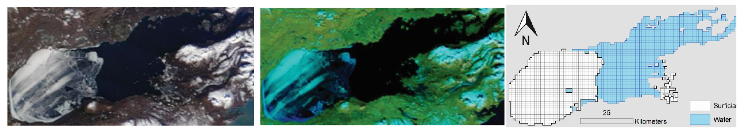
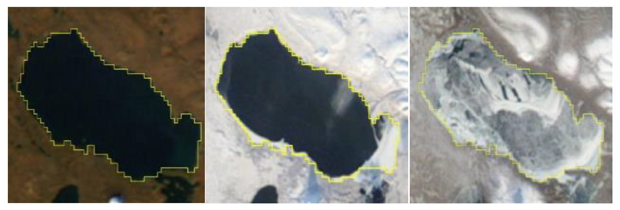
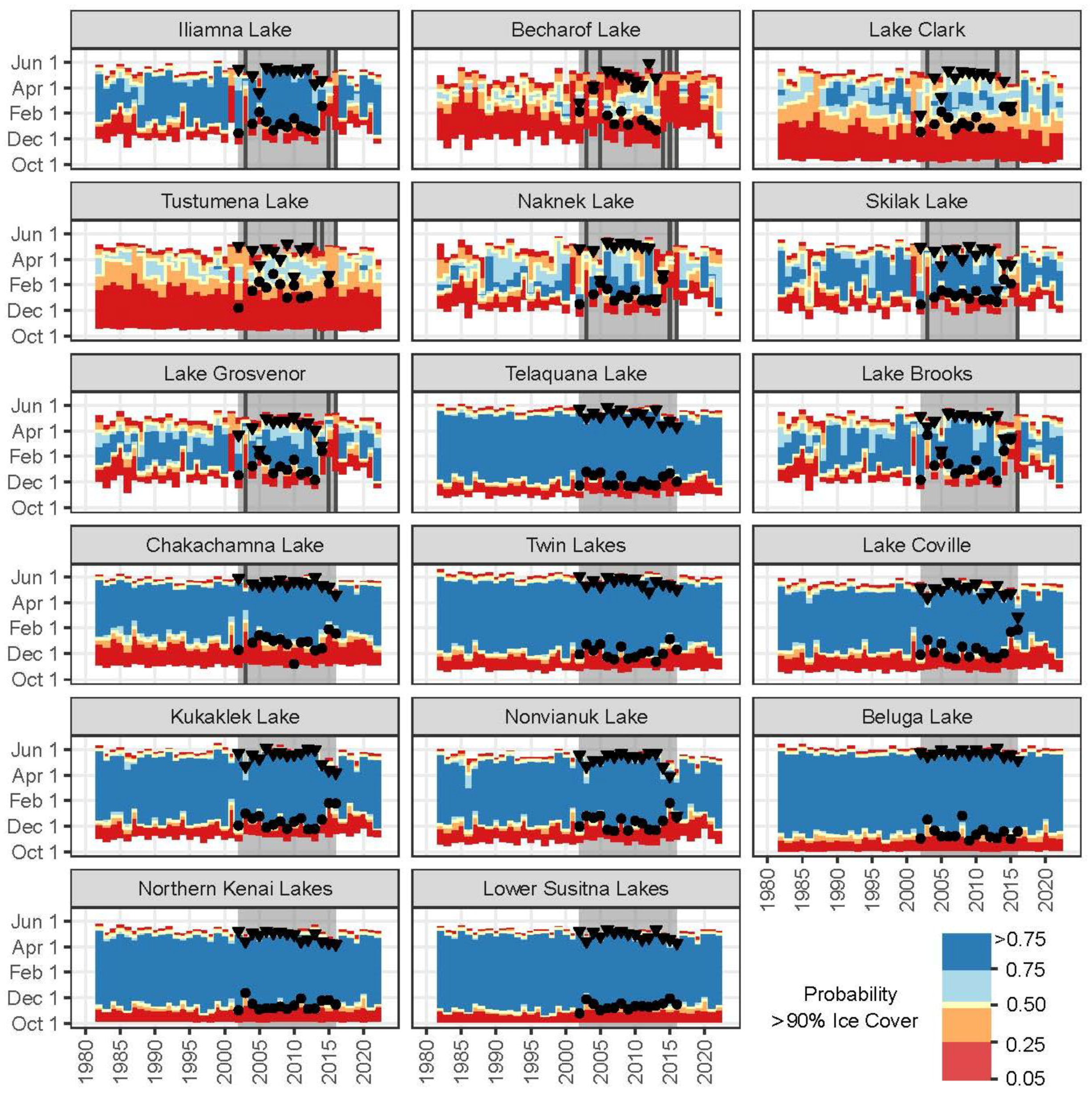
3.1. Satellite Observations
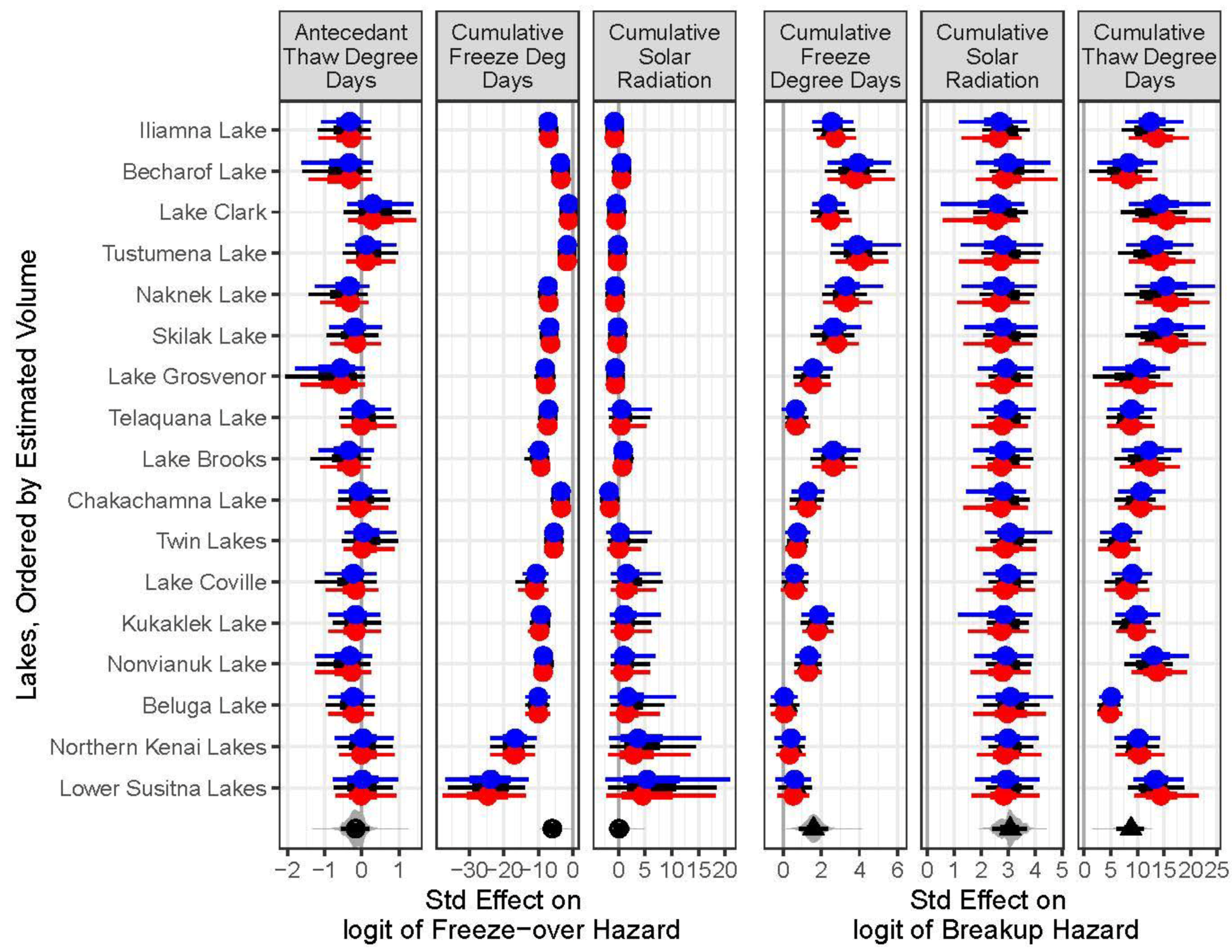
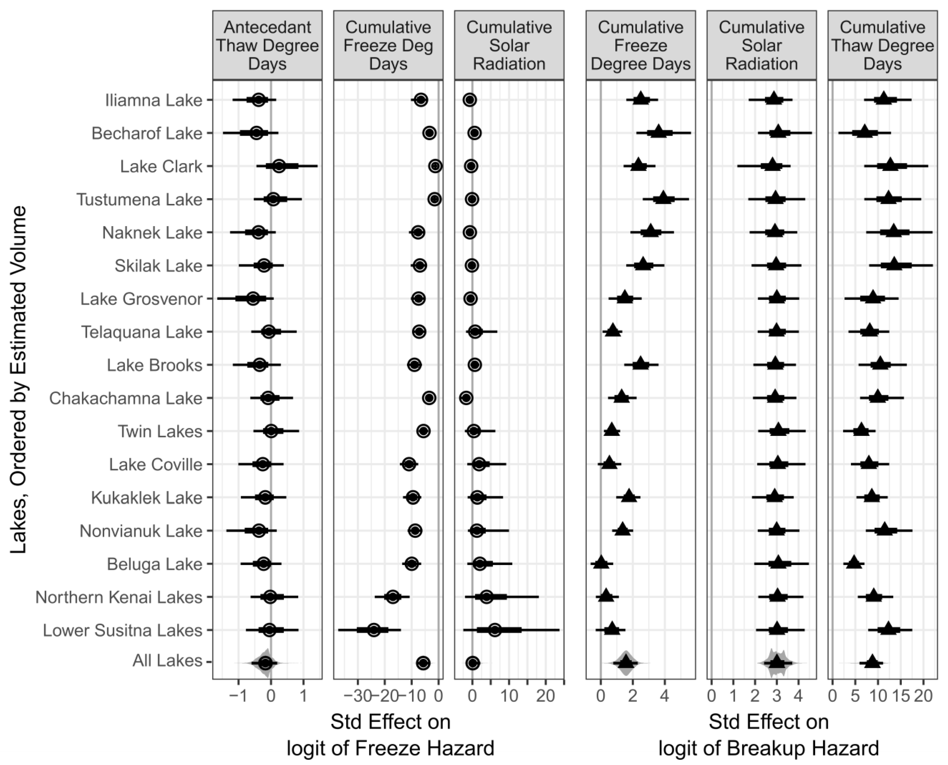
Over the 15 years of MODIS satellite observations used to calibrate our model, freeze-over (>90% ice cover) typically occurred the earliest (mid-November) in the Northern Kenai, Lower Susitna, and Beluga lakes, and the latest (late January to early February) in Becharof, Lake Clark, and Tustumena. Across all lakes, the median observed start date of freeze-over was December 20, with a MAD of 33 days. Breakup (<90% ice cover) typically occurred the earliest (late April to early May) in Becharof, Lake Clark, and Tustumena, and the latest (early June) in the highest elevation lakes—Twin Lakes and Telaquana (Figure 4). Breakup generally occurred more rapidly and the timing of breakup did not vary as greatly; the median start date of breakup was May 4, with a MAD of 19 days. The median duration of MODIS-observed ice cover > 90% was 131 days, with a MAD of 53 days. Several lakes experienced years in which >90% ice cover was not observed (Table 1).
Year-to-year variation within a given lake ranged from 7 to 27 days MAD for lake-ice formation, 10 to 80 days MAD for duration, and 4 to 22 days MAD for breakup. Scaling variation by ice-season duration revealed even greater differences. The most variable lake by this measure (Tustumena Lake) had an expected year-to-year difference in ice-season duration that exceeded its average ice-season duration by 140% (RMAD = 1.4), whereas the most consistent lake (Beluga Lake) could be expected to vary by only 6% of its average duration (RMAD = 0.06, Table 1).
In some years, multiple lakes did not freeze-over, most notably eight lakes did not freeze-over in 2003 and 2016: Iliamna, Becharof, Lake Clark, Tustumena, Naknek, Skilak, Grosvenor, and Chakachamna in 2003, and Brooks in 2016. In 2015, four lakes did not freeze-over: Iliamna, Becharof, Naknek, and Grosvenor. In 2014, two did not freeze-over: Becharof and Tustumena. In 2013, a year with sustained wind events, two did not freeze-over: Lake Clark and Tustumena (Table 1 and Figure 4). The lack of freeze-over in some years, and the interannual variability in freeze-over, duration, and breakup reflect the dynamic climate of the Southwest Alaska region during fall and early winter, which oscillates between warm and cold temperatures over several weeks and, since the 1980s, has experienced warm fall/winter temperature anomalies. The long-term variability of this cold accumulation period can be seen in the record of in situ observations from King Salmon (Figure 5) [42].

3.2. Survival Model

Our survival model for freeze-over generally fit better than our model for breakup (Figure A1 and Figure A2). Our model described 87% of the variation in freeze-over and 52% of the variation in breakup across all lakes and years. The year-to-year variance explained by the model varied substantially among lakes: from highs of 97% and 85% to lows of 47% and 24% for freeze-over and breakup, respectively. Mean absolute error varied greatly among lakes, from 5 days to 36 days with an average of 11 days for freeze-over, from 4 to 46 days with an average of 16 days for breakup, and from 6 to 41 days with an average of 19 days for duration of ice cover (Table 1, and Figure 6, Figure A1 and Figure A2).
Chilling, as measured by FDD, generally increased the freeze hazard (probability of freeze-over happening today if it has not happened already), but sensitivity to chilling varied greatly among lakes (Figure 7). We found evidence that greater antecedent summer heat loading (antTDD) decreased the freeze hazard for some lakes, but the effect was small, uncertain, and not consistently important across all lakes. Breakup hazard (probability of breakup happening today if it has not happened already) was increased at all lakes by warming (TDD) and cumulative ice-season solar radiation (SWR). Continued chilling during the ice season (FDD) decreased the breakup hazard for some lakes. Sensitivity to continued chilling was generally more pronounced in larger-volume lakes (Figure 7 and Figure 8).
The RMAD of the model-predicted ice-season duration for each lake agreed well with the RMAD of MODIS observations (Spearman rank correlation, ρ = 0.92), suggesting that the meteorologic variables that drove our model predictions could account for the observed patterns of lake variability. Our model correctly predicted 14 of 25 events when the lakes did not freeze, with one falsely predicted event. Years in which lakes did not freeze were also predicted in the anomalously warm years of the 1980s for the Becharof Lake (2), Lake Clark (2), and Tustumena Lake (6), but no non-freeze years for any other lake before 2000 (Figure 4).
We estimated decreasing trends in ice-cover duration in most, but not all, study lakes, ranging from −6 to + 2 days per decade. Over the 40 years represented in our model, nine lakes had a credibly negative trend, one lake had a credibly positive trend, and five lakes had no discernable trend. All but one lake showing a decreasing trend were <20 km3, whereas all but one lake with a positive or undiscernible trend were >20 km3 (Table 1).

3.3. Lake Volumes

Estimated lake volumes spanned four orders of magnitude, from 0.68 to >264 km3, where five of the lakes were >24 km3 (three with known volumes) and the remainder were under 7 km3. When compared to the five known volumes calculated using bathymetric measurements, we underestimated volumes in four of the lakes by 8 to 37%, and overestimated the largest lake (Lake Iliamna) by 56% (Table 1). While the volume calculations were not as precise as those made using bathymetry, considering the large differences in lake volume, this did provide a basis for an ordinal comparison that would otherwise not have been possible.
Lakes with larger estimated volumes were later to freeze-over (Spearman’s rank correlation, ρ = −0.82), had a shorter duration of ice cover (ρ = 0.82), and were less likely to freeze in years with fewer FDDs (Table 1, and Figure 4 and Figure 8). Relative variability in ice-season duration was greater in larger-volume lakes (ρ = 0.84), driven both by the tendency for large-volume lakes to be more variable in absolute terms (ρ = 0.59) and for larger-volume lakes to have shorter ice-season durations. Model-estimated sensitivity to chilling decreased with lake volume (ρ = −0.80).

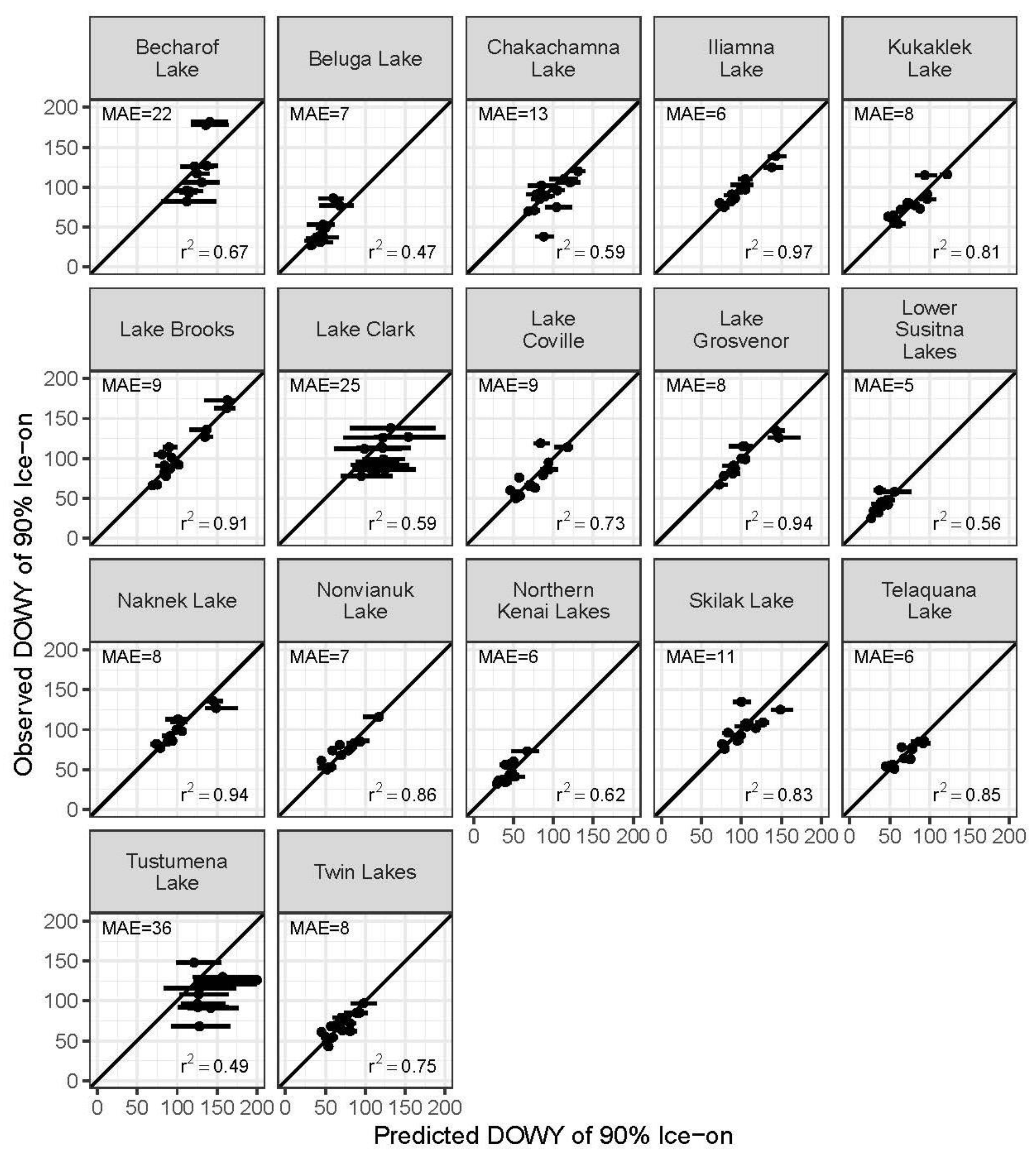
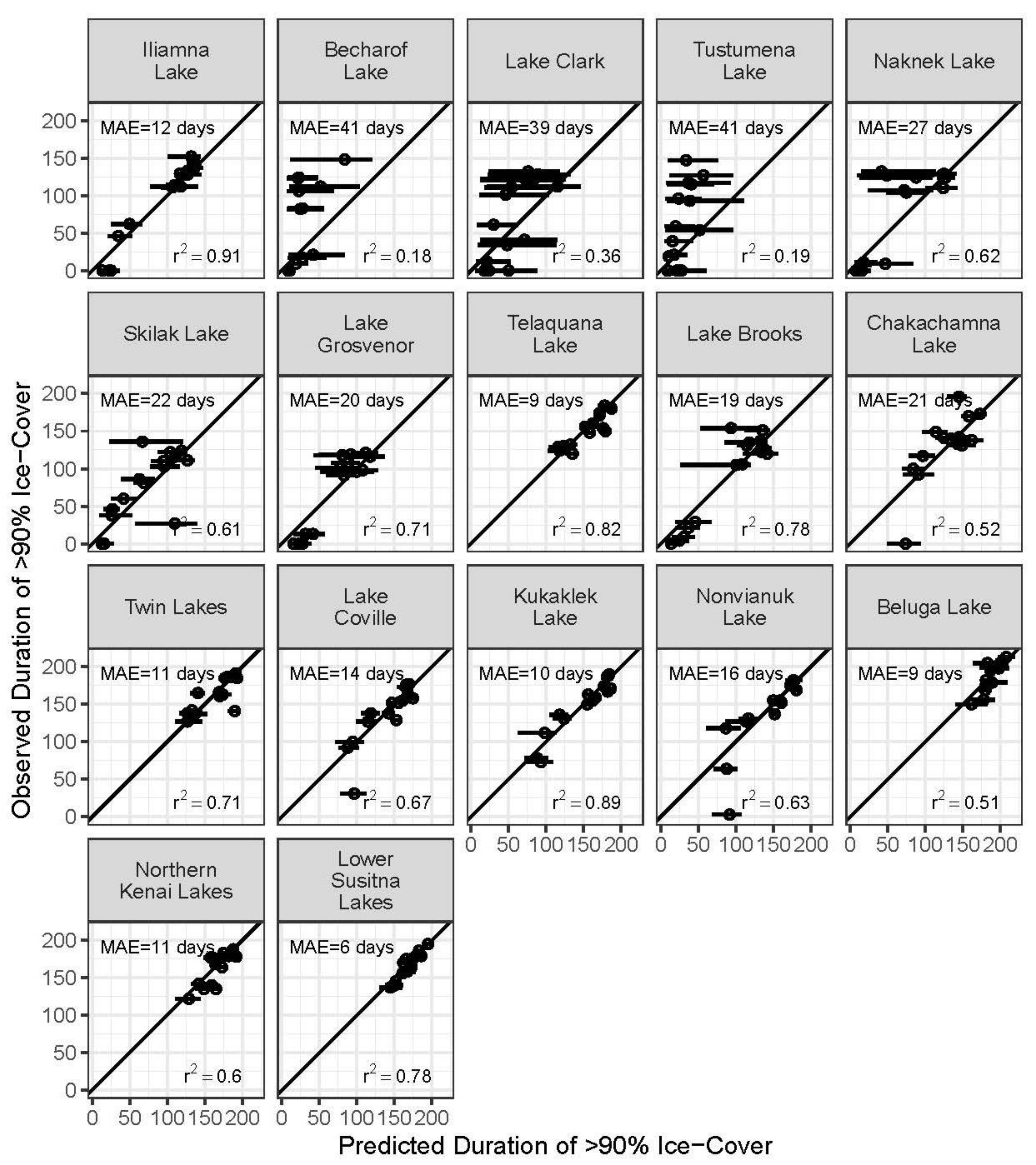
3.4. Validation against In Situ Observations

Because previous studies have found good agreement between in situ observations of lake-ice formation and melt with optical (MODIS and Sentinel) satellite remote-sensing observations, we do not present a separate validation of the satellite-observed ice season dates. Zhang et al. [43] found a MAE of 6–8 days in over 400 observations of lake-ice formation and breakup in the state of Maine in lakes that varied in size, depth, latitude, and elevation, whereas Tuttle et al. [44] found MAE of approximately 2–5 days for the ice breakup dates of a lake in Svalbard, Greenland, over a 15-year observation period.
To validate our model-predicted lake-ice seasons, we looked to available in situ observations. While there were no formal systematic observations of the percentage of ice cover for our study lakes, such as regular air photos or observers following a consistent protocol, there were three independent data sets for five lakes that were available to validate our results with. These were: (i) continuous observations of water temperature from sensor arrays deployed in three lakes, and (ii) two different long-term visual observations of ice cover for the purposes of navigating boats, snowmachines, or aircraft on two lakes.
We estimated winter stratification over sensor arrays deployed in the deepest parts of three lakes. Winter stratification can be a good indicator of ice formation in lakes that are dimictic (i.e., mix twice a year by turning over the higher-density water to depth as it heats or cools to approximately 4 °C). However, these are not always representative of ice >90% cover because the relatively small area of water directly over these locations may not be ice-covered, and the deepest parts of lakes tend to be the last to freeze. The arrays deployed in Lake Clark (100 m), Naknek (70 m), and Brooks Lake (50 m) were used to collect temperature profiles at 10 m increments over the years of 2006–2022 [45]. To estimate the duration of winter stratification, we measured the duration of time that shallow waters were cooler than deep waters by more than a mean daily temperature difference of 0.5 and 1.5 °C for the shallower (50 m) and deeper (70 and 100 m) lakes, respectively [8]. All three lakes failed to stratify in the winter of 2016, corresponding to the failure to achieve freeze-over as seen in the MODIS observations and indicated by our model results. For other years, the durations of ice cover were highly correlated (Pearson’s product moment correlation, r = 0.83–0.89, (Table 2)). Furthermore, for the years in which lake ice did not form—2013 on Lake Clark and 2015 on Naknek Lake—the overlapping temperature array data showed very short periods of stratification, which were likely not long enough for ice to form at >90% over the larger lake surface or be observed in the MODIS record.
The second set of validation data were in situ ice-cover observations for two lakes: Twin Lakes from 1982 to 1996, and Telaquana Lake from 2002 to 2020. These data were from historical observations used to record the approximate dates when the lakes would safely support foot traffic and aircraft, or were no longer navigable by boat. We again found strong correlations between the ice-cover duration derived from these observations and our modeled ice-cover duration (Twin Lakes: r = 0.95, Telaquana: r = 0.85) (Table 2).

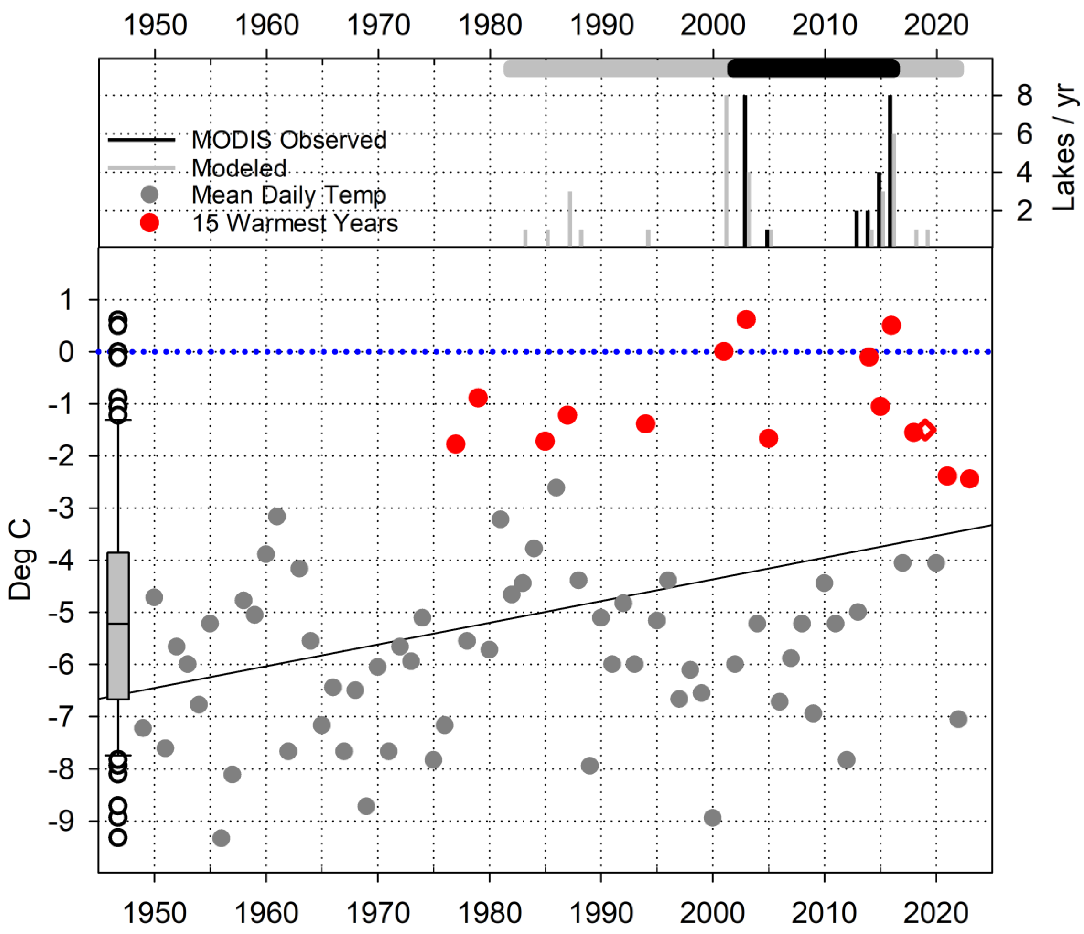
3.5. Long-Term Climate Record

Cumulative FDD in the late fall through early winter was the strongest predictor of freeze-over, and subsequently ice-cover duration, in our model (Figure 7). To consider this in the context of the regional climate record, we used the most regionally representative long-term (74 years) record of the mean daily temperatures available. We evaluated mean daily air temperatures from October 1 through February 7, with fewer than seven missing days per period, which represent the beginning and midpoint of our seasonal modeling period (Figure 5). One of the warmer years on record, 2019, was excluded due to a lack of daily observations. These data show that the 14 warmest periods between 1 October and 7 February from 1949 to 2023 have occurred since 1977. The water years of 2014, 2015, 2016, and 2018 were the 4th, 6th, 2nd, and 9th hottest years, respectively.

4. Discussion

The ecological and economic importance of lake-ice cover is widely acknowledged, but the increasing temperatures of Earth’s boreal regions have changed, and will continue to change, the patterns of lake-ice formation, duration, and breakup. However, data-intensive methods that require long-term observations and physical data are possible for only a small fraction of lakes globally. To address this, we developed a survival model to predict the historic timing and duration (phenology) of lake ice using readily accessible meteorological data and satellite-observed lake-ice cover, and hindcast predictions to explore changes over a 40-year period and evaluate them in a historic 74-year regional context.
The role of cumulative cold content through water and air temperatures has been successfully used to predict thermal stratification, mixing, and ultimately lake-ice formation by Ashton [46,47]. Likewise, cumulative heat content and “lake heatwaves” have been shown to impede the formation of lake ice [14,15,48]. Furthermore, geographic location, depth, and volume have been found to be important indicators of lake-ice dynamics [49]. Our model was developed to capture these dynamics over relevant time periods in the simplest manner possible by using geographically located predictor variables of antecedent thaw-degree days (antTDD), cumulative freezing-degree days (FDD), cumulative thaw-degree days (TDD), and cumulative downwelling shortwave radiation (SWR). The survival model and data we used revealed three broad patterns of variability, threshold response, and trend in the phenology of lake ice.

4.1. Variability

The lakes in this study vary considerably in their ice phenology, where lower-volume lakes (<20 km3) freeze-over consistently and for longer durations, and higher-volume lakes (>20 km3) freeze-over less consistently for shorter and more variable durations. The consequences of such interannual variability are best expressed when scaled by the average duration of ice cover. This relative variability revealed even more profound variation: the most variable lake (Tustumena Lake) had an expected year-to-year difference in ice-season duration that exceeded its average ice season by 140%, whereas the most consistent lake (Beluga Lake) could be expected to vary by only 6% of its average duration. Relative variability in ice-season duration was greater in larger-volume lakes, driven both by the tendency for large-volume lakes to be more variable in absolute terms and for larger-volume lakes to have shorter ice-season durations.
Interannual variation in duration of ice cover was driven more by variation in freeze-over than breakup, where freeze-over was driven primarily by chilling (accumulated FDD). Sensitivity to chilling decreased with lake volume, therefore large-volume lakes require a greater accumulation of FDD before freeze-over occurs, explaining their shorter ice-season durations (Figure 4 and Figure 8). More stable, lower-volume lakes required substantially less chilling, and reliably accumulated enough FDD to freeze early in the fall–winter season. These patterns were further affected by the lake’s location, (e.g., higher elevation and shading by surrounding terrain). Lastly, while the highest-elevation lakes (e.g., Twin, Telaquana, Chackachamna, Kukaklik, and Nonvianuk) reliably froze from year to year, there were also differences among them due to the climactic influence of the warmer Gulf of Alaska (Chackachamna) and colder interior (Telaquana) regions (Figure 1).

4.2. Threshold Response

While Lake Clark, Becharof Lake, and Tustumena Lake demonstrated non-freezing years over the duration of our study, this appears to be a new phenomenon for the other large lakes. Illiamna Lake, Nakenek Lake, Skilak Lake, Lake Grosvenor, and Brooks Lake showed little appreciable probability of a non-freezing winter in any year before 2000, but all were predicted and/or observed to not freeze in multiple winters post-2000 (Figure 9). This, coupled with fact that 12 of the 15 warmest October–February cold accumulation periods since 1949 occurred during our modeled period (1981–2021) suggests that we have reached a threshold where the expectation of several of the larger lakes freezing is substantially diminished (Figure 5 and Figure 9).
Model estimates and MODIS observations agreed on multiple years that several lakes did not freeze. Of these years, 2016 is most notable, when eight of the nine largest lakes failed to freeze-over and the mean daily temperatures were above 0 °C (Figure 4). Notably, the only large lake that did freeze in 2016 (Telaquana Lake) is the highest-elevation large lake (376 m) located in a shaded mountain valley. The 2001 and 2003 water years were also above 0 °C, with multiple lakes neither observed nor modelled to freeze-over (Figure 5 and Figure 9). The past 45 years have shown the greatest climate variability in fall/winter temperatures, with 15 of the warmest and some of the coldest years occurring since 1977 (Figure 5). These warm periods also corresponded with other climate indicators in the region, including the highest summer sea-surface temperatures of the century in the Bering Sea (2003–2005 and 2014–2020) [50], warmer waters in the Gulf of Alaska starting in 1976 [51,52], and anomalously warm waters in the Gulf for the years 2003, 2005, and 2014–2016 [53]. Benson et al. [54] and Robertson et al. [55] also recognized that large-scale atmospheric and oceanic conditions like the El Niño Southern Oscillation and the Pacific Decadal Oscillation are associated with higher winter and spring temperatures since the late 1980s, and suggest these regional climate drivers are no longer stationary [56] (Benson et al., 2011). Lastly, Dauginis [57] found consistency between declining sea ice, lake ice, and snow-on trends in Southwest Alaska.
There have only been a few detailed studies that have predicted future changes in the phenology of lake-ice cover. Dibke et al. [58] simulated lake-ice response to future climate in 2040–2079 using the CGCM3 Global Climate Model and the upper-level emission scenario (SRES A2). Their results propose that freeze-over will be later by 5–20 days, and breakup will be earlier by 10–30 days by the mid-to-late century. Lakes in Pacific coastal areas of North America saw the largest projected changes, while lakes in the Alaskan interior were less affected. More recently, Sharma et al. [9] suggested that, with continued climate warming, lakes in Southwest Alaska will experience an exponential decrease in reliable ice cover under a variety of climate scenarios.

4.3. Trend

The majority of lower-volume lakes (<10 km3) show negative trends in their period of seasonal ice cover in the order of 1–6 days per decade over our modeled period. In contrast, all but one of the lakes > 20 km3, show undiscernable or positive trends in ice-cover duration of up to two days per decade over our modeled period (Table 1).
Studies of phenology trends in northern-hemisphere lake-ice phenology have found a wide range of temporal trends that are generally negative but vary widely [9,56,57,59,60]. Our study estimated both positive and negative trends and may further explain the broad range of observed and modeled trends. The estimated trend directions were a function of (i.) the time window that we analyzed as there was a warm period near the start of our study period, and (ii.) lakes were differentially impacted by the early warm period depending on their individual characteristics. The non-negative trends were associated with a shorter duration of ice cover and a higher mean absolute error in the model fit. The trend in duration of ice cover in lakes with shorter periods of ice cover were impacted by the warm fall/winters of 85 and 87, resulting in years with short or no ice cover at the beginning of our study period, and thus a non-negative trend (Figure 4 and Figure 9). The years 1977 and 1979 were also anomalously warm, but were not covered by our modeling period. The lakes < 20 km3 in volume did not show modeled years with a short duration of ice cover in the 1980s, thus showed negative trends in duration of ice cover (Table 1).

4.4. Future Efforts

While our model accurately predicts many of the years and dates in which freeze-over and breakup occur, there are several instances where it does not. In 2013, Tustumena and Lake Clark did not freeze-over, but our model predicted they would (Figure 9). Temperature profile data available for Lake Clark in 2013 showed only eight days of winter stratification. This suggests in some years, especially on high-volume lakes with greater heat-storage capacities, other processes such as wind, seiche, and (temperature) profile mixing inhibit ice formation and exacerbate the ice breakup process due to open water and thinner ice cover.
Data collected from a meterology station near Tustumena suggest wind processes affected the ice-formation processes in 2013 when the mean October wind speed was 23% higher than the mean wind speed for October in 2001–2016 (Figure 10). Antecdotal evidence also suggests wind and waves on Lake Becharof may be a factor as well. Parts of Southwest Alaska can see particularly large atmospheric pressure gradients due to their position between the relatively shallow and cold waters of the Bristol Bay (Bering Sea) and the warmer waters of the Gulf of Alaska (Pacific Ocean). Local winds are frequently observed >30 mps (58 knots) for extended periods of time and, because Becharof has relatively flat surrounding terrain and a prevailing wind orientation, this can result in significant wave action, with wave heights of several meters on larger lakes [61]. A sustained wind can also create a seiche (water piling up downwind and later rebounding), which inhibits seasonal temperature stratification in addition to sustaining mixing on larger lakes. With sufficient data it is possible to calculate and model wind (and temperature stratification) effects on lakes of various sizes. However, given the limited availability of bathymetric profiles and local observations of wind direction and velocity, in addition to the complex topography surrounding these lakes, it is presently not possible for us to include wind in our model.
Other important variables known to affect the formation of lake-ice cover are snow cover and water chemistry. While it is possible to estimate presence or absence of snow cover using satellite data [62], we found negligeable improvement when including these data in earlier versions of our model. This suggests snowpack properties such as depth, density, and cold content, in addition to the interaction with atmospheric boundary layer conditions (e.g., vapor pressure gradients), are more important than just the presence or absence of snow [18]. Water turbidity and chemistry can also affect the process of heating, cooling, and stratification in lakes, which also affects turnover and the formation of lake ice. While several of the lakes in our study are crypto depressions (depths below sea level) (Table 1), none of them has tidal influx or evidence of seawater intrusion. Some lakes have a significant influx of glacial sediment impacting light absorption and solar heating (e.g., Lake Clark, Tustumena, Skilak, Telaquana, Chakachamna, and Twin Lakes), and others have water chemistries impacted by volcanism (Becharof) [63], but we do not suspect the addition of water quality or chemistry variables would have significantly changed our modeling results.
Because this simple model does not use difficult-to-obtain forcing variables to predict forcing variables such as wind, snow, or water quality, it should be possible to generally predict future conditions with a limited set of variables. For example, multiple Global Climate Models (GCM) that have shown good capability in predicting temperature and the first-order influences on downwelling shortwave can be statically applied. There are also efficient machine learning approaches to evaluate remote sensing data at scale that could be used for calibration [43]. This approach would be particularly useful for larger-volume lakes at lower elevations that appear to be most susceptible to small changes in accumulated FDD. However, there are tradeoffs to using this simple approach as it may miss delays in ice formation or years in which lakes do not freeze-over, as seen in our hindcast predictions when compared to MODIS observations. In cases where capturing this variability is important, additional input variables for wind and snow depth would likely improve the model skill in predicting years with intermittent forcing events of high wind, as seen for some lakes in 2013 or years when snow cover departs from the mean.

5. Conclusions

While some communities, villages, and individuals have observations of lake-ice formation and breakup at specific locations, there are very few observational datasets that describe the phenology of an entire lake, much less a robust method of predicting when ice-free conditions may occur. The types of in situ observations required for building physically based models are neither available nor financially feasible for most Alaskan stakeholders. Our open-source model addresses this by demonstrating the potential to obtain accurate probabilities of past lake-ice phenology using readily available satellite data and a few meteorologic parameters that are publicly available. Further improvements to this model could be made at a regional and local level by (i) adding wind data as a variable to the model, (ii) introducing computationally derived lake-volume estimates as a variable, and (iii) incorporating additional satellite observations and uncertainties into the modeling process. This model could also be adapted as a short- or long-term predictive tool using input variables derived from near-real time data of local weather conditions or GCMs.

Author Contributions

Conceptualization, P.B.K. and M.P.H.; methodology, M.P.H. and P.B.K.; software, M.P.H.; validation, P.B.K. and M.P.H.; formal analysis, P.B.K. and M.P.H.; investigation, P.B.K.; data Curation, P.B.K.; writing—original draft preparation, P.K; writing—review and editing, P.B.K. and M.P.H.; project administration, P.B.K. All authors have read and agreed to the published version of the manuscript.

Funding

Funding was provided by the National Park Service, Inventory and Monitoring Program, Southwest Alaska Network.

Data Availability Statement

All data used in this analysis are cited in the text and sources referenced. These data are publicly available, except for GIS bathymetry data which are pending publication and available upon request. https://irma.nps.gov/DataStore/Reference/Profile/2303056. DOI: 10.57830/2303056.

Acknowledgments

This work would not have been possible without the careful data management and image interpretation provided by the National Park Service staff including Michael Verrier, Timothy Shepherd, Chuck Lindsay, and others. Many thanks to Jim Sickman for the helpful comments and valued mentorship over the years. We also thank the reviewers who provided thoughtful insights into improving this manuscript.

Conflicts of Interest

The authors declare no conflicts of interest.

Appendix A

Detailed Model Description

We modeled lake-ice processes using a daily, discrete-time, survival modelling approach, borrowing from recent work in plant phenology. Survival models have a long history in medical research. They represent time-to-event data, allowing for events that never happen, making them well suited to modelling a process like lake-ice formation. By modelling the state of lake ice at a daily time step, we can use daily-resolved weather data to predict freeze-over and thaw-start and generate more precise predictions.
We modeled the state of lake-ice cover ( f d , y , i ) at each lake ( i in 1…17) and lake clusters on each day d of each water year y as a Bernoulli distributed random variable, with 0 representing ice cover < 90% and 1 representing ice cover > 90%:
f d , y , i Bernoulli p d , y , i
where p d , y , i is the probability of ice cover exceeding 90%. We decompose this probability into the sum of two conditional probabilities, the freeze-over hazard ( h d , y , i fr ) and the breakup hazard ( h d , y , i br ). The freeze-over hazard is the probability of ice cover exceeding 90% on day d , given that it did not by day d 1 , and the breakup hazard is the probability of ice cover dropping below 90% on day d , given that it exceeded 90% on day d 1 .
h d , y , i fr = Pr F d , y , i = 1 | F d 1 , y , i = 0 h d , y , i br = Pr F d , y , i = 0 | F d 1 , y , i = 1
p d , y , i = h d , y , i fr 1 y d 1 , y , i + 1 h d , y , i br y d 1 , y , i
We modeled the freeze-over hazard ( h d , y , i fr ) with a logistic regression: the log of the odds ratio of the hazard for lake i on day of water year d in water year y was modeled as a linear function of lake- and day-varying covariates ( F D D d , y , i , A S W R d , y , i ), and a lake- and year-varying covariate ( a n t T D D y , i ). Our model allowed for random lake-varying intercepts and regression coefficients ( β i ).
l n h d , y , i fr / 1 h d , y , i fr = β 1 , i + β 2 , i F D D d , y , i + β 3 , i S W R d , y , i + β 4 , i a n t T D D y , i
Lake-varying intercept and slope random effects were modeled as draws from a multivariate normal distribution with a mean vector µ and covariance matrix .
β 1 β 2 β 3 β 4 i M V N μ 1 β μ 2 β μ 3 β μ 4 β , Σ β
We modeled the breakup hazard ( h d , y , i br ) analogously as a logit-linear function of lake- and day-varying covariates ( T D D d , y , i , F D D d , y , i , S W R d , y , i ). For modelling the breakup hazard, d indexes days since 90% freeze-over, rather than days since start of water year.
l n h d , y , i br / 1 h d , y , i br = γ 1 , i + γ 2 , i T D D d , y , i + γ 3 , i S W R d , y , i + γ 4 , i F D D d , y , i
γ 1 γ 2 γ 3 γ 4 i M V N μ 1 γ μ 2 γ μ 3 γ μ 4 γ , Σ γ
We used weakly informative priors for all model parameters (Table A1), including a scaled Wishart distribution [31] on the covariance matrices of multivariate distributions. Priors on μ β and μ γ were chosen to aid model convergence while permitting the data to dominate the posterior distribution [64]. To assess the influence of prior probability distributions on the regression parameters, we performed a sensitivity analysis, comparing regression estimates from models where the prior variance on μ β and μ γ were 1 and 2 orders of magnitude larger. We saw only minimal differences in parameter estimates (Appendix C).
Table A1. Prior distributions for parameters in lake-ice survival models.
ParameterPrior DistributionCharacteristics
μ 1 β , μ 1 γ N 0 , 2.5 Weakly informative on logit scale
μ 2 : 4 β , μ 2 : 4 γ N 0 , 2.5 Weakly informative on logit scale
Σ β , Σ γ scaled   Wishart   s 1 : 4 = 10 , d f = 2 Uniform   for   correlation ,   half - t 2 0 , 10 for sd
From the modeled freeze-over and breakup hazards, we calculated the variables of interest in our study. “Survival”, in the case of freeze-over being the probability that lake i remained unfrozen until day d in water year w , is calculated as the product of the complement of the freeze-over hazard over all days up to and including day d :
S d , y , i fr = j = 1 d 1 H j , y , i fr
The complement of survival is the probability that freeze-over had occurred by day d in water year y :
P d , y , i fr = 1 S d , y , i fr
Similarly, the probability that lake i remained frozen d days after the date of 90% freeze-over in water year w was calculated as the product of the complement of the breakup hazard over all days from the date of freeze-over until d days after the date of freeze-over:
S d , y , i br = j = 1 d 1 H j , y , i br
and the probability that breakup had occurred by day d in water year y :
P d , y , i br = 1 S d , y , i br
The date of freeze-over and the date of breakup were estimated as the day that the probability of freeze-over and probability of breakup exceeded 0.5, respectively. Years when the probability of freeze-over did not exceed 0.5 by day 180 of the water year were classified as no-freeze years.

Appendix B

Observed versus Predicted Figures for Freeze-Over and Breakup
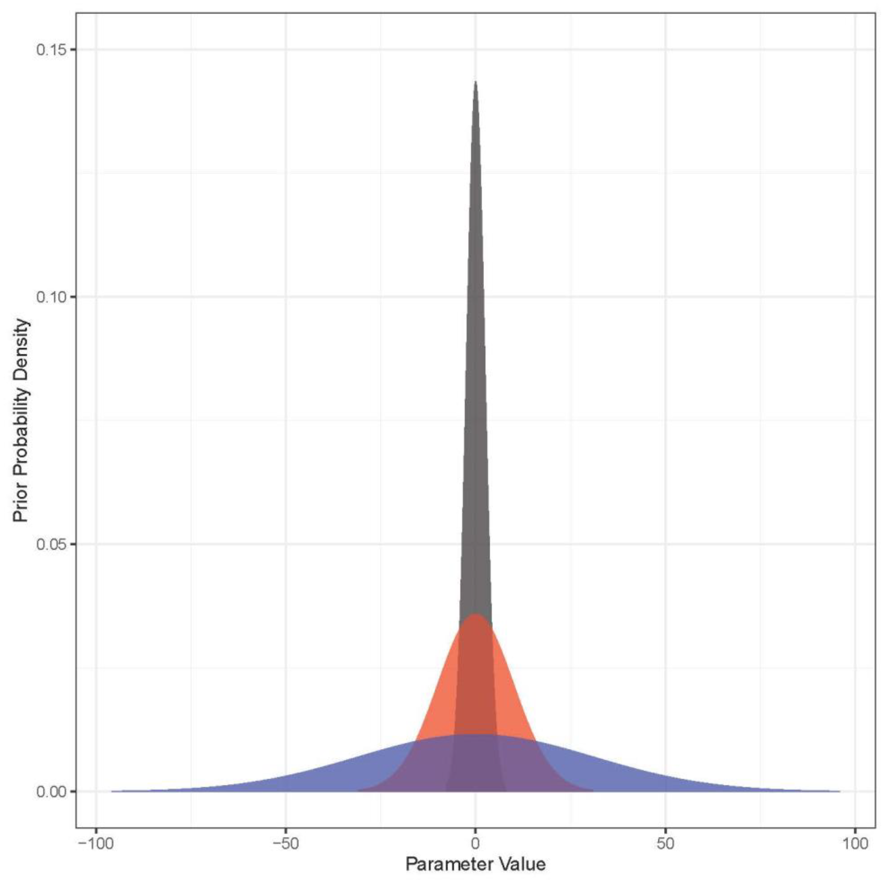
Figure A1. Model performance at each study lake. Observed versus predicted values (posterior median +/− 95% credible intervals) for freeze-over, 1:1 line in black. Mean absolute error and r2 of model predictions are shown for each lake. Higher-volume lakes are at the top of figure.
Water 16 02309 g0a1
Figure A2. Model performance at each study lake. Observed versus predicted values (posterior median +/− 95% credible intervals) for breakup, 1:1 line in black. Mean absolute error and r2 of model predictions are shown for each lake. Higher-volume lakes are at the top of figure.
Water 16 02309 g0a2

Appendix C

Appendix C.1. Bayesian Prior Sensitivity Analysis

To understand the influence that model priors might have on our inferences, we tested our prior specification against two alternate prior specifications. For the mean climate effects ( μ 2 : 4 β and μ 2 : 4 γ ), we fit models with our chosen prior, Normal (mean = 0, sd = 2.5), as well as more diffuse priors with variances covering a range of two orders of magnitude: Normal (mean = 0, sd = 10), Normal (mean = 0, sd = 31.7) (Figure A3).
Figure A3. Prior probability distributions on regression coefficients, showing the prior used in analysis, N(0, 2.5) in grey, a N(0, 10) in red, and N(0, 31.7) in blue.
Water 16 02309 g0a3
A comparison of estimated parameter values from these three models revealed minimal sensitivity of the posterior to our prior specification (Figure A4). Generally, parameter estimates in our model were constrained to be slightly smaller than in models with more diffuse priors, but the effects were small, relative to the uncertainty.
Figure A4. Model effects for model used in analysis (black) and models with alternate prior specifications, N(0, 10) in red, N(0, 31.7) in blue.
Water 16 02309 g0a4

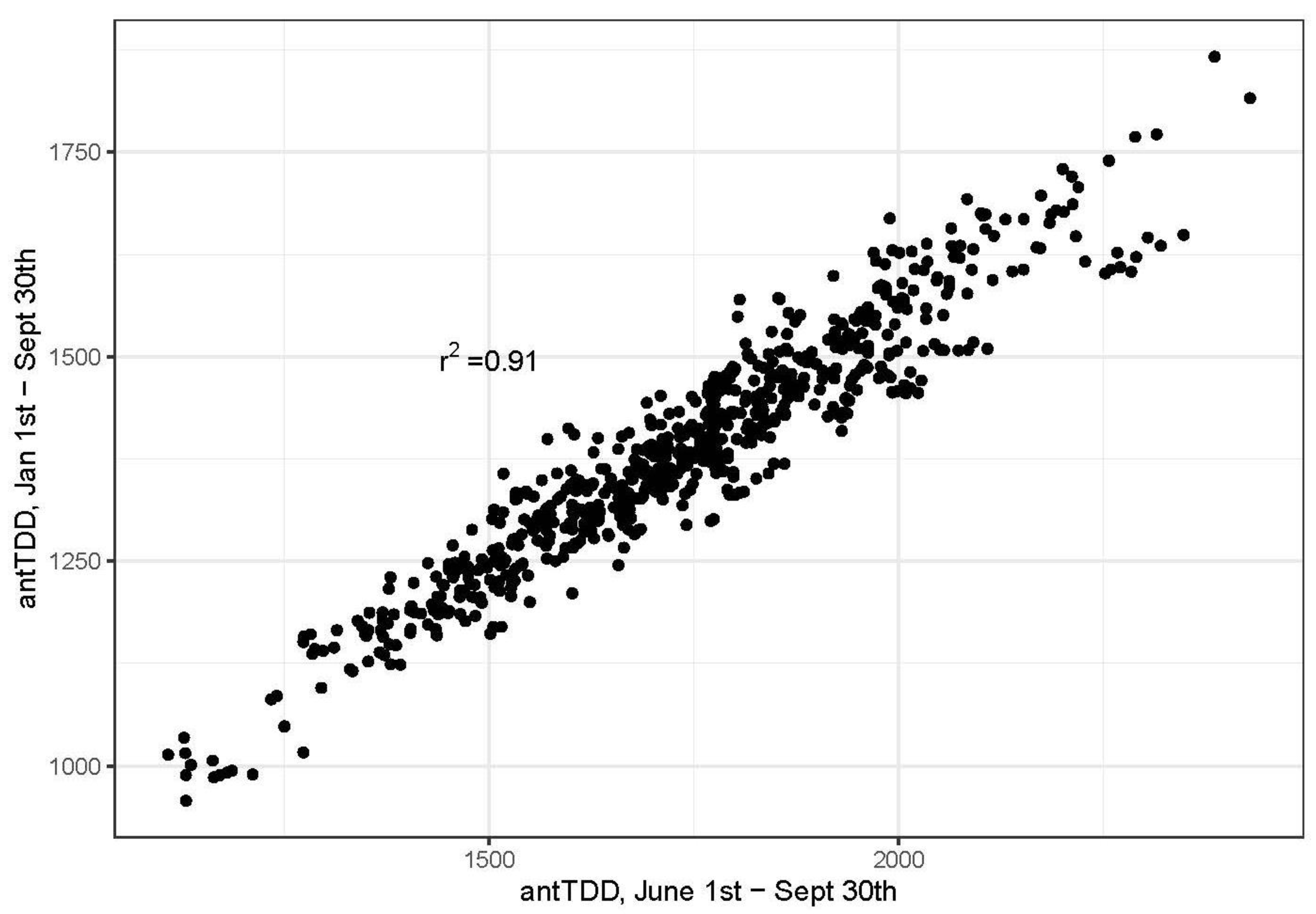
Appendix C.2. Climate Accumulation Periods

Our accumulation period for antecedent thaw-degree days (antTDD) was between June 1 and September 30. To confirm that this adequately represented the interannual variability in antTDD, we compared these values to antTDD accumulated from January 1 to September 30, predicting the latter with the former in a linear regression. This revealed that our chosen accumulation period accounted for 91% of the variability in the antTDD since the start of the calendar year (Figure A5). Furthermore, our chosen accumulation period largely avoids considering heat loading during times when the lakes may still be snow- and ice-covered, and insulated from air temperatures.
Our accumulation period for freeze-degree days (FDD) began on October 1, which accounts for most of the FDD at our study lakes. We calculated the FDD accumulated before October 1 for each lake and year of the satellite observation period. At 12 of the 17 lakes, no FDD accumulated before October 1 in any year of the satellite observation period. For the lakes that accumulated any FDD before October 1, we compared the amount accumulated by October 1 to the amount accumulated at the day of 90% freeze-over. FDD accumulated before October 1 accounted for 0–5.4% of the FDD accumulated on the day of 90% freeze-over.
Figure A5. Regression showing strong agreement between antecedent thaw-degree days (antTDD) accumulated from 1 January to 30 September vs. antTDD accumulated from 1 June to 30 September for all study lakes and years, indicating minimal potential for model sensitivity to lengthening the period of accumulation.
Water 16 02309 g0a5

References

  1. Magnuson, J.J.; Robertson, D.M.; Benson, B.J.; Wynne, R.H.; Livingstone, D.M.; Arai, T.; Assel, R.A.; Barry, R.G.; Card, V.; Kuusisto, E.; et al. Historical Trends in Lake and River Ice Cover in the Northern Hemisphere. Science 2000, 289, 1743–1746. [Google Scholar] [CrossRef] [PubMed]
  2. Newton, A.M.W.; Mullan, D.J. Climate Change and Northern Hemisphere Lake and River Ice Phenology from 1931–2005. Cryosphere 2021, 15, 2211–2234. [Google Scholar] [CrossRef]
  3. Adrian, R.; Walz, N.; Hintze, T.; Hoeg, S.; Rusche, R. Effects of Ice Duration on Plankton Succession during Spring in a Shallow Polymictic Lake. Freshw. Biol. 1999, 41, 621–634. [Google Scholar] [CrossRef]
  4. Cai, Y.; Duguay, C.R.; Ke, C.-Q. A 41-Year (1979–2019) Passive-Microwave-Derived Lake Ice Phenology Data Record of the Northern Hemisphere. Earth Syst. Sci. Data 2022, 14, 3329–3347. [Google Scholar] [CrossRef]
  5. Serreze, M.C.; Francis, J.A. The Arctic Amplification Debate. Clim. Chang. 2006, 76, 241–264. [Google Scholar] [CrossRef]
  6. Prowse, T.; Alfredsen, K.; Beltaos, S.; Bonsal, B.; Duguay, C.; Korhola, A.; McNamara, J.; Pienitz, R.; Vincent, W.F.; Vuglinsky, V.; et al. Past and Future Changes in Arctic Lake and River Ice. Ambio 2011, 40, 53–62. [Google Scholar] [CrossRef]
  7. Cohen, J.; Screen, J.A.; Furtado, J.C.; Barlow, M.; Whittleston, D.; Coumou, D.; Francis, J.; Dethloff, K.; Entekhabi, D.; Overland, J.; et al. Recent Arctic Amplification and Extreme Mid-Latitude Weather. Nat. Geosci. 2014, 7, 627–637. [Google Scholar] [CrossRef]
  8. Woolway, R.I.; Merchant, C.J. Worldwide Alteration of Lake Mixing Regimes in Response to Climate Change. Nat. Geosci. 2019, 12, 271–276. [Google Scholar] [CrossRef]
  9. Sharma, S.; Blagrave, K.; Magnuson, J.J.; O’Reilly, C.M.; Oliver, S.; Batt, R.D.; Magee, M.R.; Straile, D.; Weyhenmeyer, G.A.; Winslow, L.; et al. Widespread Loss of Lake Ice around the Northern Hemisphere in a Warming World. Nat. Clim. Chang. 2019, 9, 227–231. [Google Scholar] [CrossRef]
  10. Gaul, K. Nanutset ch’u Q’udi Gu, before Our Time and Now, An Ethnohistory of Lake Clark National Park and Preserve. USDOI, NPS, Lake Clark National Park and Preserve, 179. 2007. Available online: https://nps.gov/lacl/learn/historyculture/upload/Nanutset-Gaul-508.pdf (accessed on 20 October 2023).
  11. Cold, H.S.; Brinkman, T.J.; Brown, C.L.; Hollingsworth, T.N.; Brown, D.R.N.; Heeringa, K.M. Assessing Vulnerability of Subsistence Travel to Effects of Environmental Change in Interior Alaska. Ecol. Soc. 2020, 25, 20. [Google Scholar] [CrossRef]
  12. Bogdanova, E.; Lobanov, A.; Andronov, S.V.; Soromotin, A.; Popov, A.; Skalny, A.V.; Shaduyko, O.; Callaghan, T.V. Challenges of Changing Water Sources for Human Wellbeing in the Arctic Zone of Western Siberia. Water 2023, 15, 1577. [Google Scholar] [CrossRef]
  13. Bengtsson, L.; Herschy, R.W.; Fairbridge, R.W. (Eds.) Ice Formation on Lakes and Ice Growth. In Encyclopedia of Lakes and Reservoirs; Springer: Dordrecht, The Netherlands, 2012. [Google Scholar]
  14. Leppäranta, M. Modelling the Formation and Decay of Lake Ice. In The Impact of Climate Change on European Lakes; George, G., Ed.; Springer Science & Business Media: Dordrecht, The Netherlands, 2009; Volume 4. [Google Scholar]
  15. Leppäranta, M. Ice Phenology and Thickness Modelling for Lake Ice Climatology. Water 2023, 15, 2951. [Google Scholar] [CrossRef]
  16. Kirillin, G.; Leppäranta, M.; Terzhevik, A.; Granin, N.; Bernhardt, J.; Engelhardt, C.; Efremova, T.; Golosov, S.; Palshin, N.; Sherstyankin, P.; et al. Physics of Seasonally Ice-Covered Lakes: A Review. Aquat. Sci. 2012, 74, 659–682. [Google Scholar] [CrossRef]
  17. Launiainen, J.; Cheng, B. Modelling of Ice Thermodynamics in Natural Water Bodies. Cold Reg. Sci. Technol. 1998, 27, 153–178. [Google Scholar] [CrossRef]
  18. Brown, L.C.; Duguay, C.R. A Comparison of Simulated and Measured Lake Ice Thickness Using a Shallow Water Ice Profiler. Hydrol. Process. 2011, 25, 2932–2941. [Google Scholar] [CrossRef]
  19. Rafat, A.; Pour, H.K.; Spence, C.; Palmer, M.J.; MacLean, A. An Analysis of Ice Growth and Temperature Dynamics in Two Canadian Subarctic Lakes. Cold Reg. Sci. Technol. 2023, 210, 103808. [Google Scholar] [CrossRef]
  20. Golub, M.; Thiery, W.; Marcé, R.; Pierson, D.; Vanderkelen, I.; Mercado, D.; Woolway, R.I.; Grant, L.; Jennings, E.; Schewe, J.; et al. A framework for ensemble modelling of climate change impacts on lakes worldwide: The ISIMIP Lake Sector. Geosci. Model Dev. Discuss. 2022, 15, 4597–4623. [Google Scholar] [CrossRef]
  21. Wynne, R.H. Statistical Modeling of Lake Ice Phenology: Issues and Implications. SIL Proc. 2000, 27, 2820–2825. [Google Scholar] [CrossRef]
  22. Preston, D.L.; Caine, N.; McKnight, D.M.; Williams, M.W.; Hell, K.; Miller, M.P.; Hart, S.J.; Johnson, P.T.J. Climate Regulates Alpine Lake Ice Cover Phenology and Aquatic Ecosystem Structure. Geophys. Res. Let. 2016, 43, 5353–5360. [Google Scholar] [CrossRef]
  23. Beyene, M.T.; Jain, S.; Gupta, R.C. Linear-Circular Statistical Modeling of Lake Ice-Out Dates. Water Resour. Res. 2018, 54, 7841–7858. [Google Scholar] [CrossRef]
  24. Terres, M.A.; Gelfand, A.E.; Allen, J.M.; Silander, J.A. Analyzing First Flowering Event Data Using Survival Models with Space and Time-varying Covariates. Environmetrics 2013, 24, 317–331. [Google Scholar] [CrossRef]
  25. Diez, J.M.; Pulliam, H.R. Hierarchical Analysis of Species Distributions and Abundance Across Environmental Gradients. Ecology 2007, 88, 3144–3152. [Google Scholar] [CrossRef] [PubMed]
  26. Elmendorf, S.C.; Crimmins, T.M.; Gerst, K.L.; Weltzin, J.F. Time to Branch out? Application of Hierarchical Survival Models in Plant Phenology. Agric. For. Meteorol. 2019, 279, 107694. [Google Scholar] [CrossRef]
  27. USGS Publications Warehouse, 1992, 1:2,000,000-Scale Digital Line Graph (DLG) Data. Available online: https://pubs.usgs.gov/publication/ds4 (accessed on 30 July 2009).
  28. McCabe, S.; Bartz, K.; Young, D.; Gabriel, P. GIS bathymetry of selected southwest Alaska Lakes, from field measurements. In GIS Data Layer, in Preparation; National Park Service Southwest Alaska Inventory and Monitoring Network: Anchorage, AK, USA, 2024. [Google Scholar]
  29. U.S. Bureau of Reclamation. Chakachamna Project, Alaska Status Report; Alaska District Office: Juneau, AK, USA, 1962; 21p. [Google Scholar]
  30. Spafard, M.A.; Edmonson, J.A. A Morphometric Atlas of Alaskan Lakes: Cook Inlet, Prince William Sound, and Bristol Bay Areas; Alaska Department of Fish and Game, Commercial Fisheries Division: Anchorage, AK, USA, 2000. Available online: www.adfg.alaska.gov/fedaidpdfs/RIR.2A.2000.23.pdf (accessed on 20 June 2024).
  31. Hollister, J.; Milstead, W.B. Using GIS to Estimate Lake Volume from Limited Data. Lake Reserv. Manag. 2010, 26, 194–199. [Google Scholar] [CrossRef]
  32. Reed, B.; Budde, M.; Spencer, P.; Miller, A.E. Integration of MODIS-Derived Metrics to Assess Interannual Variability in Snowpack, Lake Ice, and NDVI in Southwest Alaska. Remote Sens. Environ. 2009, 113, 1443–1452. [Google Scholar] [CrossRef]
  33. Verrier, M.; Shepherd, T.; Spencer, P.; Lindsay, C.; Kirchner, P. Southwest Alaska Remote Sensing Lake Ice Phenology for 17 Lakes and Lake Clusters for 2002–2016 Water Years; National Park Service—Southwest Alaska Inventory and Monitoring Network: Anchorage, AK, USA, 2024. [Google Scholar] [CrossRef]
  34. Thorton, M.M.; Shrestha, R.; Wei, Y.; Thornton, P.E.; Kao, S.-C.; Wilson, B.E. Daymet: Daily Surface Weather Data on a 1-km Grid for North America, Version 4R1; ORNL DAAC: Oak Ridge, TN, USA, 2022. [Google Scholar] [CrossRef]
  35. Plummer, M. JAGS Version 4.3.0 User Manual 2017, 73. Available online: https://sourceforge.net/projects/mcmc-jags/ (accessed on 20 September 2023).
  36. Kellner, K. jagsUI: A Wrapper around “rjags” to Streamline “JAGS” Analyses 2018. Available online: https://CRAN.R-project.org/package=jagsUI (accessed on 1 April 2024).
  37. Kay, M. Tidybayes: Tidy Data and Geoms for Bayesian Models 2022. Available online: https://mjskay.github.io/tidybayes/ (accessed on 1 April 2024).
  38. R Core Team. R: A Language and Environment for Statistical Computing 2019. Available online: https://R-project.org/ (accessed on 20 September 2023).
  39. Gelman, A.; Rubin, D.B. Inference from Iterative Simulation Using Multiple Sequences. Stat. Sci. 1992, 7, 457–511. [Google Scholar] [CrossRef]
  40. Gelman, A.; Goodrich, B.; Gabry, J.; Vehtari, A. R-Squared for Bayesian Regression Models. Am. Stat. 2019, 73, 307–309. [Google Scholar] [CrossRef]
  41. Nakagawa, S.; Schielzeth, H. A General and Simple Method for Obtaining R2 from Generalized Linear Mixed-effects Models. Methods Ecol. Evol. 2012, 4, 133–142. [Google Scholar] [CrossRef]
  42. Eggleston, K. xmACIS Version 1.0.69a, NOAA Northeast Regional Climate Center Released 4-Dec-2023. Available online: https://xmacis.rcc-acis.org (accessed on 1 May 2023).
  43. Zhang, S.; Pavelsky, T.M. Remote Sensing of Lake Ice Phenology across a Range of Lakes Sizes, ME, USA. Remote Sens. 2019, 11, 1718. [Google Scholar] [CrossRef]
  44. Tuttle, S.E.; Roof, S.R.; Retelle, M.J.; Werner, A.; Gunn, G.E.; Bunting, E.L. Evaluation of Satellite-Derived Estimates of Lake Ice Cover Timing on Linnévatnet, Kapp Linné, Svalbard Using In-Situ Data. Remote Sens. 2022, 14, 1311. [Google Scholar] [CrossRef]
  45. Bartz, K.; Gabriel, P. Lake Temperature Monitoring in Southwest Alaska Parks: A Synthesis of Year-Round, Multi-Depth Data from 2006 through 2018; National Park Service: Fort Collins, CO, USA, 2020. [Google Scholar] [CrossRef]
  46. Ashton, G.D. Lake Ice Decay. Cold Reg. Sci. Technol. 1983, 8, 83–86. [Google Scholar] [CrossRef]
  47. Ashton, G.D. River and Lake Ice Thickening, Thinning, and Snow Ice Formation. Cold Reg. Sci. Technol. 2011, 68, 3–19. [Google Scholar] [CrossRef]
  48. Woolway, R.I.; Albergel, C.; Frölicher, T.L.; Perroud, M. Severe Lake Heatwaves Attributable to Human-Induced Global Warming. Geophys. Res. Lett. 2022, 49, e2021GL097031. [Google Scholar] [CrossRef]
  49. Zhou, J.; Leavitt, P.R.; Rose, K.C.; Wang, X.; Zhang, Y.; Shi, K.; Qin, B. Controls of Thermal Response of Temperate Lakes to Atmospheric Warming. Nat. Commun. 2023, 14, 6503. [Google Scholar] [CrossRef] [PubMed]
  50. Huang, B.; Thorne, P.; Banzon, V.; Boyer, T.; Chepurin, G.; Lawrimore, J.; Menne, J.; Smith, T.; Vose, S.; Zhang, H. NOAA Extended Reconstructed Sea Surface Temperature (ERSST), Version 5. NOAA National Centers for Environmental Information. 2017. Available online: https://ncei.noaa.gov/access/ (accessed on 29 December 2023).
  51. Hartmann, B.; Wendler, G. The Significance of the 1976 Pacific Climate Shift in the Climatology of Alaska. J. Clim. 2005, 18, 4824–4839. [Google Scholar] [CrossRef]
  52. Litzow, M.A.; Mueter, F.J. Assessing the Ecological Importance of Climate Regime Shifts: An Approach from the North Pacific Ocean. Prog. Oceanogr. 2014, 120, 110–119. [Google Scholar] [CrossRef]
  53. Danielson, S.L.; Hennon, T.D.; Monson, D.H.; Suryan, R.M.; Campbell, R.W.; Baird, S.J.; Holderied, K.; Weingartner, T.J. Temperature Variations in the Northern Gulf of Alaska across Synoptic to Century-Long Time Scales. Deep-sea Research. Part 2. Topical Studies in Oceanography/Deep Sea Research. Part II Top. Stud. Oceanogr. 2022, 203, 105155. [Google Scholar] [CrossRef]
  54. Benson, B.J.; Magnuson, J.J.; Jacob, R.L.; Fuenger, S.L. Response of Lake Ice Breakup in the Northern Hemisphere to the 1976 Interdecadal Shift in the North Pacific. Verh. Int. Ver. Theor. Angew. Limnol. 2000, 27, 2770–2774. [Google Scholar] [CrossRef]
  55. Robertson, D.M.; Wynne, R.H.; Chang, W.Y.B. Influence of El Niño on Lake and River Ice Cover in the Northern Hemisphere from 1900 to 1995. Verh. Int. Ver. Theor. Angew. Limnol. 2000, 27, 2784–2788. [Google Scholar] [CrossRef]
  56. Benson, B.J.; Magnuson, J.J.; Jensen, O.P.; Card, V.M.; Hodgkins, G.; Korhonen, J.; Livingstone, D.M.; Stewart, K.M.; Weyhenmeyer, G.A.; Granin, N.G. Extreme Events, Trends, and Variability in Northern Hemisphere Lake-Ice Phenology (1855–2005). Clim. Chang. 2011, 112, 299–323. [Google Scholar] [CrossRef]
  57. Dauginis, A.A.; Brown, L.C. Recent Changes in Pan-Arctic Sea Ice, Lake Ice, and Snow-on/off Timing. Cryosphere 2021, 15, 4781–4805. [Google Scholar] [CrossRef]
  58. Dibike, Y.; Prowse, T.; Saloranta, T.; Ahmed, R. Response of Northern Hemisphere Lake-ice Cover and Lake-water Thermal Structure Patterns to a Changing Climate. Hydrol. Process. 2011, 25, 2942–2953. [Google Scholar] [CrossRef]
  59. Weyhenmeyer, G.A.; Livingstone, D.M.; Meili, M.; Jensen, O.; Benson, B.; Magnuson, J.J. Large Geographical Differences in the Sensitivity of Ice-Covered Lakes and Rivers in the Northern Hemisphere to Temperature Changes. Global Chang. Biol. 2010, 17, 268–275. [Google Scholar] [CrossRef]
  60. Wang, X.; Feng, L.; Qi, W.; Cai, X.; Zheng, Y.; Gibson, L.; Tang, J.; Song, X.; Liu, J.; Zheng, C.; et al. Continuous Loss of Global Lake Ice Across Two Centuries Revealed by Satellite Observations and Numerical Modeling. Geophys. Res. Lett. 2022, 49, e2022GL099022. [Google Scholar] [CrossRef]
  61. Warren, K.; Margaret, W. U.S. Fish & Wildlife Service, Region 7, Water Resources Branch, Egegik River/Becharof Lake Watershed Navigability Research Report, October 1997. Available online: https://dnr.alaska.gov/mlw/paad/nav/rdi/gegik_becharof/becharof_draft_report.pdf (accessed on 21 February 2024).
  62. Lindsay, C.; Zhu, J.; Miller, A.E.; Kirchner, P.; Wilson, T.L. Deriving Snow Cover Metrics for Alaska from MODIS. Remote Sens. 2015, 7, 12961–12985. [Google Scholar] [CrossRef]
  63. LaPerriere, J.D. Limnological Monitoring of Lake Becharof, Final Report to the U.S. Fish and Wildlife Service, Research Work Order 58, Alaska Cooperative Fish and Wildlife Research Unit April l998. Available online: https://ecos.fws.gov/ServCat/DownloadFile/108087 (accessed on 15 February 2024).
  64. Gelman, A.; Jakulin, A.; Pittau, M.G.; Su, Y.S. A Weakly Informative Default Prior Distribution for Logistic and Other Regression Models. Ann. Appl. Stat. 2008, 2, 1360–1383. [Google Scholar] [CrossRef]
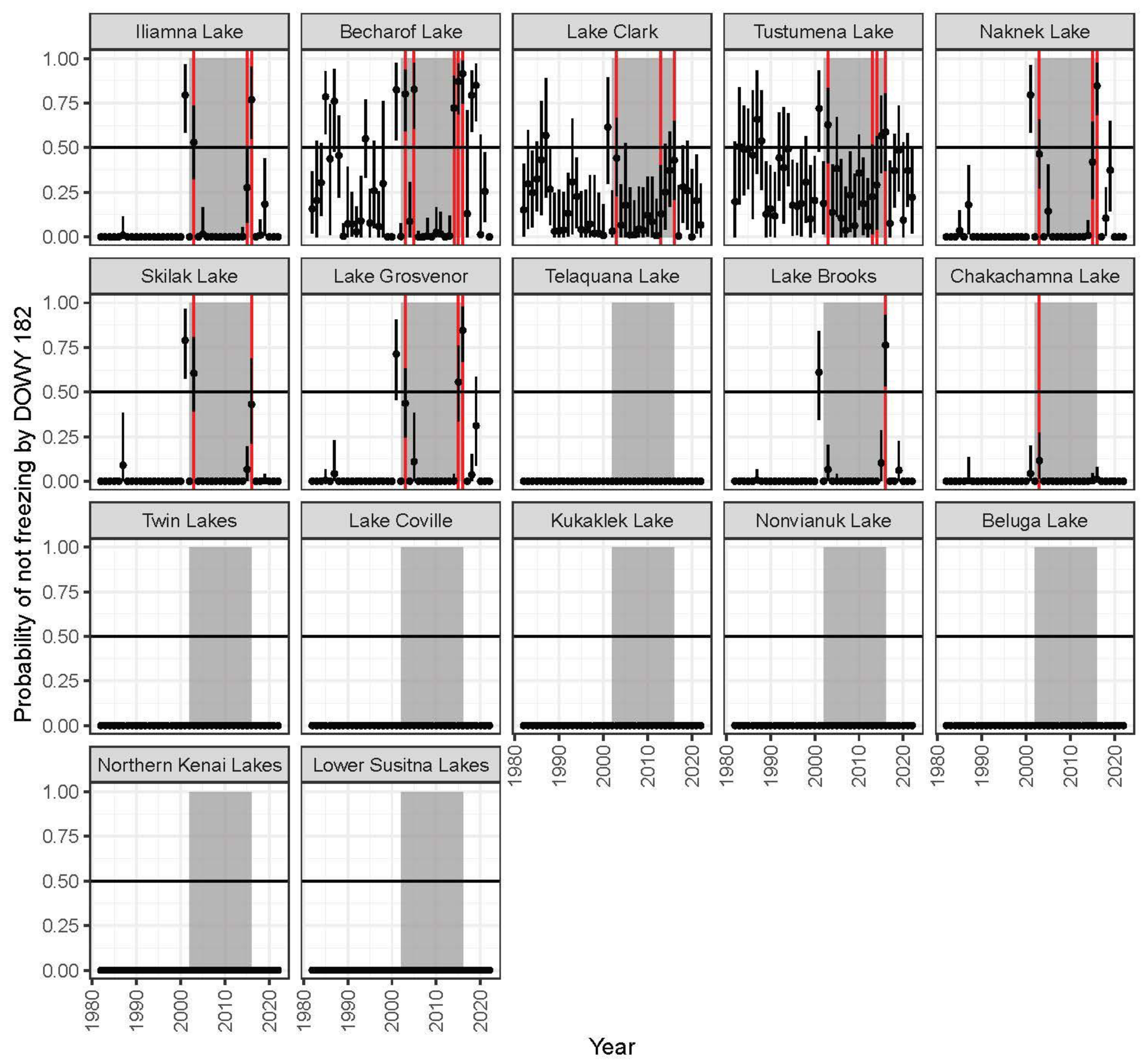
Figure 1. Location of study area, lake number refer to lake names and metrics listed in Table 1.
Water 16 02309 g001
Figure 2. MODIS image classification for Lake Iliamna 25 February 2015. True color (bands 1, 4, 3) (left), NIR and SWIR (bands 7, 2, 1) (middle), and estimation of percentage of ice cover using grid mask (right).
Water 16 02309 g002
Figure 3. Examples of metric thresholds from Lake Becharof. MODIS true color images with no ice cover on October 11, 14% on December 23, and 92% (freeze-over) on February 15.
Water 16 02309 g003
Figure 4. Modeled and observed ice cover. Modeled probability of ice cover > 90% by lake, for period of study, with observed MODIS dates of 90% freeze-up (black circles) and breakup (black triangles). The period of interpreted satellite observation is spanned by the light grey background, and years in which the lakes did not freeze are marked by dark grey vertical background bars. The highest-volume lakes are at the top of the figure.
Water 16 02309 g004
Figure 5. 1949 to 2022 regional record of King Salmon airport daily mean air temperatures during the fall/winter cold-accumulation period. Lower panel shows the 15 warmest periods (red), where 4 show a mean above or near 0 °C (dotted blue line) since the early 2000s (2019 had insufficient data, and the diamond represents nearby station). Upper panels’ vertical bars show the number of lakes observed by MODIS (black) and modeled (grey) for each year that lakes did not fully freeze-over; the horizontal bars show the years of observation and modeling in this study. The boxplot on the left shows the high variance of data and predominance of years during the observation and modeling periods relative to all years.
Water 16 02309 g005
Figure 6. Model performance at each study lake. Observed versus predicted values (posterior median +/− 95% credible intervals) for the duration of ice cover, 1:1 line in black. Mean Absolute Error and r2 of model predictions are shown for each lake. Higher-volume lakes are at the top of figure.
Water 16 02309 g006
Figure 7. Meteorologic variables’ effects on freeze-start (circles, left 3 panels) and breakup (triangles, right 3 panels). Each panel shows the effect of a 1-sd change in the predictor variable on the log of the odds-ratio of the hazard, where the freeze hazard is the probability of 90% or more ice cover occurring today, given less than 90% ice cover yesterday, and the breakup hazard is the probability of less than 90% ice cover today, given greater than 90% ice cover yesterday. Model coefficients are estimated by their posterior medians (points) +/− 95% credible intervals (thin bars) and 66% credible intervals (thick bars). Greater magnitude coefficients indicate a stronger relationship or greater apparent sensitivity to a meteorologic variable. Higher-volume lakes are at the top.
Water 16 02309 g007
Figure 8. Freeze degree day (FDD) accumulation. Cumulative FDD before freeze-over shown in blue, after freeze-over shown in grey, date of freeze-over indicated by dot. The years in which our model indicated that lakes did not freeze by March-30 are shown in red. Higher volume lakes are at the top of figure.
Water 16 02309 g008
Figure 9. Modeled probability of ice cover exceeding 90%. Vertical red lines show the 0.5 probability of each lake reaching the 90% ice cover by March 30, (DWY 18). Black points and error bars show the posterior median (+/− 95% credible intervals) and the grey rectangles show the years of MODIS observations. Higher-volume lakes are at the top of figure.
Water 16 02309 g009
Figure 10. Wind rose comparisons. In 2013, lake ice was prevented from forming on Lake Clark and nearby Tustumena Lake. Winds observed from Soldotna, close to Lake Tustemena, demonstrate the average annual wind direction and intensity for October 2002–2016 water years (left) and the 2013 water year (right) when the average wind speed was 29% higher. (Data from Western Regional Climate Center).
Water 16 02309 g010
Table 1. Lake Characteristics.
Lake AArea km2Lake Elev. mMax. Depth m BConical Volume est. km3Known Volumes km3No-Freeze Years n = 15
MODIS C
No-Freeze Years n = 40
Model D
Duration Trend Days/Year EMAD Days F RMAD G
1  Iliamna Lake263711301264.58115.336−0.5 * [−0.8,−0.2]400.43
2  Becharof Lake119549236.6544.05110.2 * [0.0,0.6]310.57
3  Lake Clark3367526629.7932.3330.2 [−0.8,0.8]460.63
4  Tustumena Lake2983429028.81-4110.2 [−0.4,0.9]801.35
5  Naknek Lake4581316024.43-460.2 [−0.1,0.5]330.44
6  Skilak Lake99581745.747.222−0.1 [−0.1,−0.4]530.69
7  Lake Grosvenor73351122.73-33−0.2 [−0.2,−0.4]300.40
8  Telaquana Lake483761322.112.900−0.5 * [−0.7,−0.1]230.21
9  Lake Brooks7520822.05-120.0 [−0.3,0.4]250.28
10 Chakachamna74346801.97-10−0.1 [−0.8,0.4]150.11
11 Twin Lakes276011030.93-00−0.5 * [−0.8,−0.2]330.20
12 Lake Coville3335620.68-00−0.6 * [−0.7,−0.3]310.23
13 Kukaklek Lake173247---00−0.6 * [−0.7,−0.4]200.23
14 Nonvianuk Lake133191---00−0.6 * [−0.7,−0.4]340.24
15 Beluga Lake4475---00−0.3 * [−0.5,−0.2]100.06
16 Northern Kenai8860---00−0.3 * [−0.5,−0.1]160.10
17 Lower Susitna6139---00−0.6 * [−0.9,−0.3]150.09
Notes: A Lake number corresponds with Figure 1 ordered by relative volume, where max depth was available; B maximum lake-depth estimates, lakes in cryptodepressions; C number of no-freeze observations in 15-year MODIS record; D number of years of <50% probability of freeze in 40-year model run; E positive and negative trends in duration of freeze (* credibly different from 0) [with upper and lower terciles]; F MAD (variation) of MODIS-observed duration of ice cover; G RMAD (relative variation) of MODIS-observed duration of ice cover.
Table 2. Model compared to in situ observations.
Lake Validation Data AYears BModel
Correlation
Mean Duration Obs.Mean Duration ModelSD Obs.SD Modeln YearsConical Volume EstimateRanking by Proxy Volume
Lake ClarkT, Array, 100 m2006–2022 0.84606047271629.793
Naknek LakeT, Array, 70 m2008–2022 0.89877445471424.435
Telaquana LakeIce obs.2002–2020 *0.851501572121122.737
Lake BrooksT, Array, 50 m2010–2022 0.8373774644122.059
Twin LakesIce obs.1982–1996 *0.951771721712140.9311
Notes: A Type of in-situ observations (and array depth) used for validation. B Asterisk indicates data had a gap in one or more years of ice observation.
Disclaimer/Publisher’s Note: The statements, opinions and data contained in all publications are solely those of the individual author(s) and contributor(s) and not of MDPI and/or the editor(s). MDPI and/or the editor(s) disclaim responsibility for any injury to people or property resulting from any ideas, methods, instructions or products referred to in the content.

