Predicting Arsenic Contamination in Groundwater: A Comparative Analysis of Machine Learning Models in Coastal Floodplains and Inland Basins

Abstract

Arsenic (As) contamination in groundwater represents a major global health threat, potentially impacting billions of individuals. Elevated As concentrations are found in river floodplains across south and southeast Asia, as well as in the inland basins of China, despite varying sedimentological and hydrogeochemical conditions. The specific mechanisms responsible for these high As levels remain poorly understood, complicating efforts to predict and manage the contamination. Applying hydro-chemical, geological, and soil parameters as explanatory variables, this study employs multiple linear regression (MLIR) and random forest regression (RFR) models to estimate groundwater As concentrations in these regions. Additionally, random forest classification (RFC) and multivariate logistic regression (MLOR) models are applied to predict the probability of As levels exceeding 10 μg/L in the Hetao Basin (China) and Bangladesh. Model validation reveals that RFR explains 80% and 70% of spatial variability of As concentration in the Hetao Basin and Bangladesh, respectively, outperforming MLIR, which accounts for only 35% and 32%. Similarly, RFC outperforms MLOR in predicting high As probability, achieving correct classification rates of 98.70% (Hetao Basin) and 98.25% (Bangladesh) on training datasets, and 82.76% (Hetao Basin) and 91.20% (Bangladesh) on validation datasets. The performance of the MLOR model on the validation set yields accuracy rates of 81.60% and 72.18%, respectively. In the Hetao Basin, Ca²⁺, redox potential (Eh), Fe, pH, SO₄²⁻, and Cl⁻ are key predictors of As contamination, while in Bangladesh, soil organic carbon (SOC), pH, and SO₄²⁻ are significant predictors. This study underscores the potential of random forest (RF) models as robust tools for predicting groundwater As contamination.

1. Introduction

Geogenic arsenic (As) contamination in groundwater is a pressing global environmental health issue, particularly affecting south and southeast Asian countries [1,2,3]. Despite extensive research [4,5,6], the mechanisms driving As mobilization and the prediction of its concentrations remain elusive due to irregular distribution of As and the limited availability of data. Consequently, there is a critical need for the development of reliable prediction methods [7,8]. Elevated As levels are typically found in flat, low-lying sedimentary aquifers from the Late Pleistocene to Holocene periods [9,10]. Potential geochemical processes responsible for high As concentrations include reductive dissolution of As-bearing iron oxides under reducing conditions, oxidative dissolution of As-bearing pyrite in oxic environments, and As desorption driven by pH changes and competitive ion interactions [11]. These primary release mechanisms are influenced by various hydrological and biogeochemical factors [12,13], with geographical variations further complicating As contamination patterns. Consequently, predicting groundwater As contamination is challenging due to the interplay of multiple factors such as pH, redox potential (Eh), ionic composition, and mineral type [14] and is difficult to predict using a single parameter.

Inland basins, typically the Datong, the Hetao, and the Huhhot Basins in North China, exhibit widespread As contamination. Previous studies demonstrate that elevated As concentrations occurred resulting from Fe oxide dissolution under reducing conditions [15], sulfide mineral weathering, and cation exchange processes [16]. Additionally, historical mining activities may have contributed to As transport downstream [17]. Similarly, floodplains, especially in Bangladesh, Cambodia, and Pakistan, have high-As groundwater. Previous studies indicate that elevated As concentrations occurred resulting from redox changes involving the reduction of Fe-oxyhydroxides and subsequent oxidation [18,19,20]. Furthermore, HCO₃⁻ presence and elevated pH levels can mobilize As from minerals and sediments [21,22]. Overall, inland basins and floodplains exhibit different yet overlapping As contamination mechanisms. Previous studies [23,24] typically relied on hydro-chemical or geological data for predicting As contamination in a single area, either in inland basins or flood Basins. A combination of hydrogeochemical and geological data and simultaneously predicting groundwater As contamination in those two regions could provide insight for understanding mechanisms to control As contaminations.

Accurate and precise estimates of groundwater As contamination is essential for effective pollution controls. Various modeling techniques, such as artificial neural networks (ANN), multiple linear regression (MLIR), random forest (RF), and principal component regression (PCR), have been widely used for contamination forecasting [25,26,27,28]. While MLIR is commonly employed for predicting As concentrations, its linear nature and difficulty in capturing outliers often result in lower accuracy [29,30]. In this context, MLIR and MLOR models are now commonly employed as benchmarks to assess the performance of alternative models. These models set the baseline for the minimum acceptable accuracy in various studies [31]. For example, RF models generally demonstrate superior performance compared to MLIR and MLOR models [32,33]. Despite this, MLIR remains a valuable tool; for instance, it has shown better performance than ANN in predicting water quality indices in Nigeria [34]. Additionally, research has indicated that decision trees (DT), used in isolation, can achieve greater accuracy and efficiency compared to PCR, with RF representing an ensemble of such decision trees, demonstrating even greater efficacy over DT [35,36]. In contrast, random forest regression (RFR) offers several advantages, including the ability to establish nonlinear relationships, handle categorical and continuous variables, prevent overfitting, and provide unbiased error rate measurements [37]. These characteristics make RFR particularly suitable for complex environmental datasets. Few studies have demonstrated the effectiveness of RFR in predicting As contamination in groundwater [38,39]. Furthermore, implementing binary classification could offer valuable insights into the presence or absence of contamination, thus supporting more targeted and efficient mitigation strategies. However, binary classification methods have not been extensively explored in As contamination predictions. In this study, MLIR and RFR models were utilized to predict As concentrations in groundwater. Additionally, multivariate logistic regression (MLOR) and random forest classification (RFC) methods were applied to assess the probability of high As contamination (>10 μg/L) in the Hetao Basin and Bangladesh. The objectives were to: (i) model and predict As contamination in the Hetao Basin and Bangladesh using MLIR, RFR, MLOR, and RFC by incorporating hydro-chemical, soil, and geological data; (ii) evaluate and compare the performance of these models in forecasting groundwater As concentrations; and (iii) identify and analyze differences in As contamination patterns between the Hetao Basin and Bangladesh.

2. Materials and Methods

2.1. Study Area

The Hetao Basin is located between the Yellow River and the Langshan Mountains (Figure 1). The Langshan Mountains, which rise up to 2365 m above mean sea level (m asl), bound the basin to the northwest. These mountains were uplifted by a normal fault along the mountain front, which originated at the end of the Jurassic period and remained active until the end of the Late Pleistocene, with a fault slope of 60–70°. The Langshan Mountains consist primarily of a metamorphic complex [40], encompassing Jurassic to Cretaceous metamorphic sedimentary rocks (sandstone, mudstone, and shale) and Mesoproterozoic metamorphic rocks (quartz slate, quartzite, phyllite, marble, schist, and two-mica schist), as well as intrusive rocks (granite and diorite). Tectonic movements have folded and fractured these complex Cenozoic sedimentary rocks, including conglomerate and sandstone, which outcrop in the valleys. During the Tertiary period, red or deep brown sedimentary rocks formed under oxic conditions [41], serving as the primary source of sediments for the adjacent flat plain.

Alluvial fans have developed near the mountain valleys due to the deposition of pluvial sediments, extending from the mountain ranges to a broad plain with gradients between 1/100 and 1/150. The flat plain, covering 75% of the study area, features gradients between 1/1000 and 1/5000 and contains 1500 to 8000 m of sediments. Pluvial sediments, primarily gravel and coarse to medium sand, are found in the alluvial fans, while inland lacustrine sediments, composed of silt and fine sand, were locally deposited in the plain during the Quaternary period [42]. Groundwater is mainly found in Quaternary alluvial, alluvial-pluvial, and alluvial-lacustrine aquifers. The alluvial-pluvial unconfined aquifers are predominant in the belt of alluvial fans, whereas fluvial-lacustrine leaky-confined aquifers are common in the flat plain [43].

Figure 1. Spatial distribution of groundwater As concentrations in the Hetao Basin (data from [16,44]).

Figure 1. Spatial distribution of groundwater As concentrations in the Hetao Basin (data from [16,44]).

The Bengal delta plain, one of the largest deltas globally, has been shaped by sediment deposition from the Ganges–Meghna–Brahmaputra (GMB) river system (Figure 2). The Bangladesh encompasses most of the Bengal delta plain, with a portion extending into West Bengal. The Pleistocene uplands in northwest Bangladesh are known as the Barind Tract, while the central region contains the Madhupur Tract. These areas feature the characteristic brown Madhupur Clay and Dupi Tila sands, remnants of uplifted blocks from periods of low sea level. The Ganges–Brahmaputra–Meghna rivers transport an estimated annual sediment load of several 10¹² kg, with about one-third deposited in the subaerial delta and floodplain [45]. The substantial influx of detritus from the eroded ultramafic, granitic, and high-grade metamorphic rocks of the Himalayas’ northern, central, and southern regions is the primary source of dominant minerals such as quartz, biotite, and feldspar [46]. In the Bengal Delta, alluvial deposits of silt, clay, sand, and gravel, typically 30–80 m thick, have accumulated over the past 5–7 thousand years of the Holocene, unconformably overlying the Pleistocene fluvio-deltaic sediments. These Pleistocene sediments, comprising oxidized mud and sand layers, were tectonically uplifted and are associated with several active NE–SW faults. Sediment types deposited in the delta have been significantly influenced by global sea level changes during Pleistocene glaciations [45,47].

2.2. Hydrogeochemical Data Collecting and Processing

Studies indicate that high As concentrations in groundwater are generally influenced by hydrogeochemical, geological, and soil factors [11]. The interaction between surface water and groundwater, precipitation, and human activities can also influence As concentration [46,49,50,51]. The selection of hydrogeochemical and soil-related parameters is based on their direct influence on the concentration and behavior of As in groundwater. Hydrogeochemical parameters, such as pH, oxidation-reduction potential (Eh), and the presence of specific ions like calcium (Ca²⁺), chloride (Cl⁻), and sulfate (SO₄²⁻) are crucial as they directly affect the mobility and speciation of arsenic. Soil properties, including organic carbon density (OCD), clay content (CC), soil organic carbon (SOC), bulk density (BD), silt content (SC), and cation exchange capacity (CEC), play significant roles in arsenic retention and release in the soil-water system. These parameters determine the adsorption capacity of soils, influencing how arsenic is transported through the subsurface environment.

By considering these hydrogeochemical and soil-related parameters, we aim to capture the primary factors that control arsenic distribution in groundwater, providing a robust basis for predicting arsenic concentrations. While other factors like surface water interactions, precipitation, and human activities also play roles, our focus on these parameters ensures a comprehensive understanding of the natural geochemical processes governing arsenic behavior in groundwater systems.

To predict groundwater As concentrations, we utilized As concentration data from groundwater wells in the Hetao Basin and three regions in Bangladesh (Rajshahi, Dhaka, and Chittagong). The As datasets for Bangladesh were sourced from [48], encompassing data collected from 1997 to 2001. Data for the Hetao Basin were obtained from [44] and [16], with As concentrations measured during field campaigns in July 2007 and July 2017. The study area in the Hetao Basin is divided into three zones: the alluvial fan, the transitional zone, and the plain zone. Water table levels in the alluvial fan are approximately 20 m below the land surface (BLS), while in the plain zone, groundwater levels drop to about 1 m BLS [44]. Ref. [16] reported groundwater levels ranging from 13 to 32 m BLS, with an average of 23 m BLS. In comparison, Ref. [48] documented groundwater levels ranging from 3.6 to 37.5 m BLS, with an average of 24.5 m BLS [48]. Regarding the concern about the comparability of hydrochemical data collected at different times, we argue that groundwater in these regions is highly stable over time. This stability ensures that using data from different periods is reasonable and reliable for predicting As concentrations. This inherent stability in groundwater characteristics allows for robust comparisons and analyses across datasets collected at different times. Hydrogeochemical data including Ca²⁺, Cl⁻, DOC, Eh, Mg, pH, and SO₄²⁻ were included within these As datasets. Additional geological and soil properties, including OCD, CC, SOC, BD, SC, and CEC, were acquired from SoilGrids (https://soilgrids.org/). The spatial resolution of the SoilGrids data is 250 m. The geological cross sections of the two areas are shown in Figure S1 and Figure 2.

After collecting the data, the first step involves removing any missing or blank entries to ensure the dataset’s integrity and reliability. This preprocessing step is crucial for eliminating noise and potential biases that could affect subsequent analyses. Once the dataset is cleaned, it is then processed and analyzed according to the three sigma (3σ) rule [52]. After applying the 3σ rule, a comprehensive statistical analysis is performed on the refined dataset. This analysis includes calculating key statistical metrics such as the maximum value, minimum value, mean, and variance. These metrics provide a detailed summary of the data distribution and variability, offering insights into the central tendency and dispersion of the data.

With the statistical groundwork laid, the next phase involves conducting modeling analysis. This process is systematic and methodical, adhering to a predefined sequence of methods as illustrated in Figure 3. Each step in this sequence builds upon the previous one, ensuring a robust and thorough evaluation of the data. The modeling methods are chosen based on their relevance and applicability to the specific characteristics of the dataset, aiming to extract meaningful patterns and relationships.

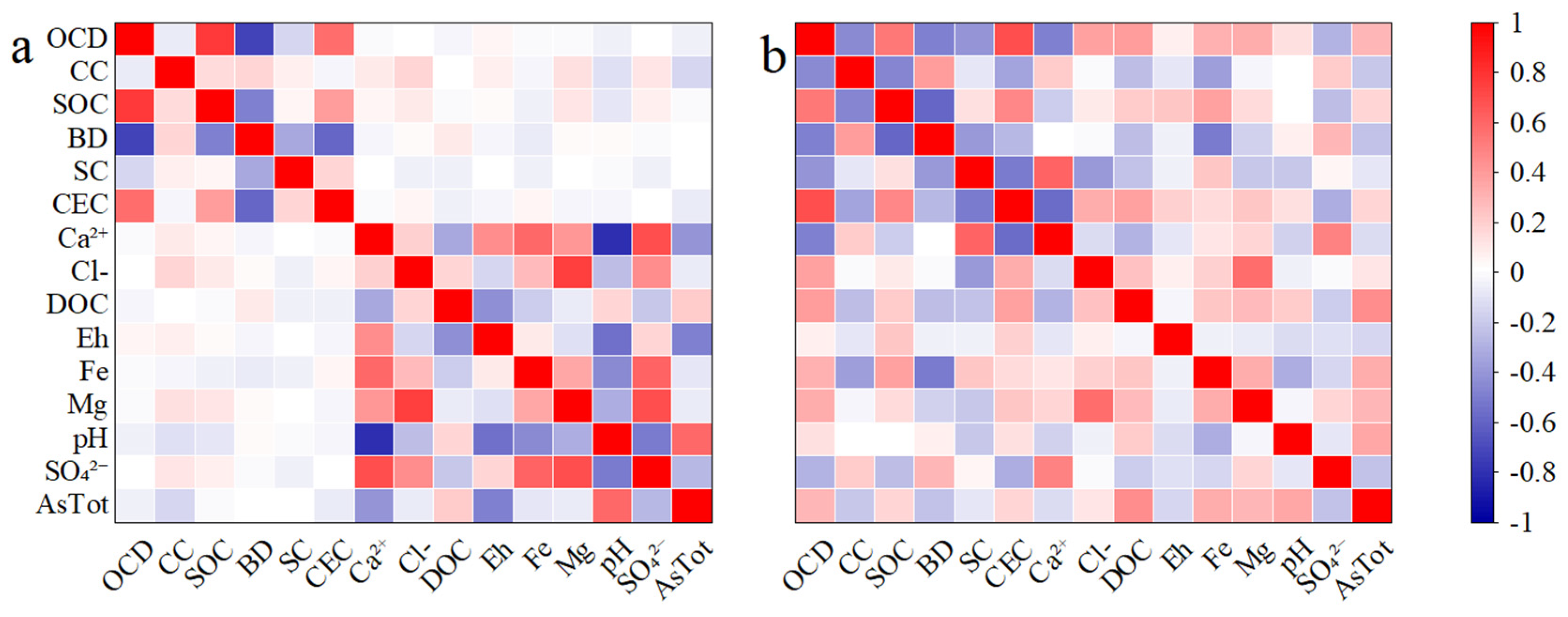
2.3. Multicollinearity Assessment

In this study, two methods were employed to assess the relationships among the selected factors: Variance Inflation Factor (VIF) with a threshold of less than 10, and Pearson’s Correlation Coefficients (r) not exceeding ±0.7 [53]. If the VIF and r values are >10 and >±0.7, respectively, this indicates significant collinearity issues. The VIF analysis revealed that the highest value was 9.4 (Table S1), indicating that all values were within the acceptable range (VIF < 10). This suggests that multicollinearity is not a significant concern, allowing us to confidently include all examined features in the model without risking inflated standard errors or misleading parameter estimates. The Pearson Correlation plot, shown in Figure 4, and the corresponding values listed in Tables S2 and S3 demonstrate a maximum correlation of 0.70 and a minimum of −0.63, which are within the acceptable standard of r ≤ ±0.7. These results indicate that none of the predictors are highly correlated with each other, further reducing the likelihood of multicollinearity affecting the model’s performance.

These assessments influenced the final model selection by ensuring that only variables with acceptable levels of collinearity were included. By confirming that both VIF and r values are within the acceptable ranges, we established a robust foundation for the model. This careful selection process enhances the reliability and validity of the model’s predictions, ensuring that the estimated coefficients are unbiased and that the model’s interpretability is maintained. Consequently, this approach eliminates the possibility of false significance. For instance, if Feature 1 is significant for As concentration but also significantly correlated with Feature 2, leading to the incorrect conclusion that Feature 2 is also significant for As concentration, our method prevents such misleading outcomes [54].

2.4. Feature Selections for Models

For MLIR, we assessed the significance of independent variables using p-values, considering a threshold of 0.05 to indicate significant correlations. Variables identified as significant (p < 0.05) parameters in

Table 1. Results of multiple linear regression (MLIR) model.

Hetao Basin
Predictor Variables	Coefficients	Standard Error	Standardized Coefficients	p Value
intercept	−2312.778	836.709	/	0.007
OCD	−0.887	1.291	−0.137	0.493
CC	−0.852	0.649	−0.094	0.192
SOC	1.062	0.808	0.162	0.191
BD	−1.031	3.225	−0.047	0.75
SC	−0.052	0.521	−0.011	0.92
CEC	−0.461	0.742	−0.054	0.536
Ca²⁺	0.718	0.578	0.18	0.216
Cl−	−0.031	0.071	−0.051	0.657
DOC	6.54	3.934	0.134	0.099
Eh	−0.25	0.244	−0.101	0.307
Fe	85.617	31.68	0.254	0.008
Mg	0.68	0.511	0.179	0.186
pH	349.246	67.566	0.679	<0.001
SO42−	−0.201	0.1	−0.24	0.047
Bangladesh
Predictor Variables	Coefficients	Standard Error	Standardized Coefficients	p Value
intercept	−877.873	598.590	/	0.145
OCD	0.102	0.383	0.033	0.790
CC	−1.427	2.995	−0.037	0.634
SOC	−0.486	2.850	−0.015	0.865
BD	0.075	0.342	0.026	0.826
SC	−0.034	0.215	−0.024	0.874
CEC	−0.981	0.596	−0.170	0.102
Ca2⁺	−0.225	0.281	−0.092	0.424
Cl−	−0.156	0.090	−0.141	0.086
DOC	10.117	2.981	0.244	0.001
Eh	−0.052	0.101	−0.034	0.605
Fe	10.207	2.554	0.338	<0.001
Mg	2.005	0.669	0.275	0.003
pH	173.960	32.274	0.379	<0.001
SO₄²−	−0.784	0.427	−0.144	0.069

were used in the MLIR model to predict As contamination. In the Hetao Basin, the significant predictors were pH, Fe, and SO₄²⁻, while significant predictors were pH, Mg, Fe, and DOC in Bangladesh. For the RFR model, we employed feature combination optimization to minimize the root mean square error (RMSE) and determine the optimal combination of predictive variables [55]. Various combinations of hydro-chemical, geological, and soil parameters were tested, and the RMSE value in the validation phase was used to identify the best model. The optimal predictive variables for the Hetao Basin were determined to be Ca²⁺, Eh, Fe, pH, SO₄²⁻, and Cl⁻, whereas for Bangladesh, the optimal predictors were SOC, pH, and DOC.

Furthermore, for MLOR and RFC, we utilized a variable selection method based on r [56,57]. This method involves: (i) starting with the variables with the highest positive or negative r from the available dataset, and (ii) gradually adding variables with lower r until the variable with the lowest r is included. The goal was to determine whether the variable with the highest r alone could accurately predict the outcome or if additional variables were necessary for optimal prediction. Models were evaluated based on RMSE values in the validation phase to determine the best variable combination. Ultimately, MLOR identified pH, Fe, and SO₄²⁻ as the optimal predictors for the Hetao Basin, highlighting the significant role of these factors in the region’s environmental conditions. For Bangladesh, pH, Mg, Fe, and DOC were the significant predictors, indicating the diverse influences of geologic conditions and water chemistry in this area. On the other hand, RFC determined Ca²⁺, Fe, pH, SO₄²⁻, and Cl⁻ as the best predictors for the Hetao Basin. This suggests that the combination of these variables captures the complexity of the environmental interactions more effectively for this region. For Bangladesh, RFC determined SOC, pH, and DOC as the optimal predictors, underlining the importance of soil organic content and chemical properties in this context.

The feature importance plots (Figure S3) visually represent the significance of each variable in the RF models. These plots clearly show the dominance of certain variables, with pH and DOC consistently emerging as crucial factors across different regions and models. The consistency of pH as a significant predictor underscores its fundamental role in influencing environmental processes. Similarly, the importance of DOC in both regions indicates its critical function in soil and water chemistry dynamics.

RF is a machine learning algorithm that creates multiple decision trees and aggregates their results to produce a final output [58]. Generally, a higher number of decision trees improves model performance. However, excessive decision trees can lead to overfitting, diminishing the model’s reliability [59]. To prevent this, we restricted the number of decision trees in the RFR and RFC models to a maximum of 100. The optimal number of trees is determined by selecting the quantity that maximizes the R² coefficient for RFR and the accuracy rate for RFC.

2.5. Adopted Modeling Approach and Validation

This study employed two predictive models, RFR and MLIR, to forecast As contamination. The RFC and MLOR approaches were used to develop a predictive model for assessing probability of high or low risk based on a specified As threshold. To date, these methods have been widely used in research on groundwater As contamination [39,60]. The models utilized raw As concentration values for RFR and MLIR, while RFC and MLOR used binary-coded data points: contaminated (As ≥ 10 µg/L, coded as 1) or uncontaminated (As < 10 µg/L, coded as 0). These analyses were conducted using the Python programming language [61]. For model construction and validation, sampling points were randomly split into two subsets: 80% of the samples were used to build the model, and the remaining 20% were used for validation. The MLOR model uses a set of $x$ independent variables to predict the response variable $\mathrm{Y}$, which in this study represents the As concentration. This model is formulated as shown in Equation (1),

$$\mathrm{Y} ={\beta }_0+{\beta }_1{x}_1+{\beta }_2{x}_2+{\beta }_3{x}_3+{\beta }_4{x}_4+\mathrm{Є}$$

(1)

where Y is a dependent variable; x₁, x₂, x₃, and x₄ are the independent variables; β₀ is the y intercept; β₁, β₂, β₃, and β₄ are the slope; and $\mathrm{Є}$ is a random error.

The sigmoid function is represented by Equation (2) as follows:

$$\mathrm{P} =1/1+{ \mathrm{e}}^{-y}$$

(2)

Apply the sigmoid function in Equation (3) as follows:

$$P=1/1+e^{-\left({\beta }_0+{\beta }_1{x}_1+{\beta }_2{x}_2+{\beta }_3{x}_3+{\beta }_4{x}_4\right)}$$

(3)

For the evaluation of models, RFR and MLIR use the coefficient of determination (R²) of the regression model, and RFC and MLOR employ three statistical validation techniques and one graphical technique: operating characteristics (ROC) curve, Correct Classification Rate, False Negative Rate, and False Positive Rate. The AUC (area under the ROC curve) ranges from 0.5 to 1, with values closer to 1 indicating better model performance [62]. These metrics are used to assess accuracy [63], calculated as follows:

$$\mathrm{AUC} ={\displaystyle \frac{\left(\mathsf{\Sigma }TP+\mathsf{\Sigma }\mathrm{TN}\right)}{\left(P+N\right)}}$$

(4)

$$Correct Classification Rate={\displaystyle \frac{TP+TN}{TP+TN+FP+FN}}$$

(5)

$$False Negative Rate={\displaystyle \frac{FN}{TP+FN}}$$

(6)

$$False Positive Rate= {\displaystyle \frac{FP}{TN+FP}}$$

(7)

where TP, TN, FP, and FN interpret the true positive, true negative, false positive, and false-negative accordingly, and N is the total number of samples.

3. Results and Discussion

3.1. Hydro-Chemical and Geological Characteristics of Groundwater in the Hetao Basin and Bangladesh

This study compares groundwater hydrogeochemical and geological characteristics between the Hetao Basin in China and three regions in Bangladesh (Rajshahi, Dhaka, and Chittagong). Key geological parameters include OCD, CC, SOC, BD, SC, CEC (

Table 2. Descriptive statistics of the variables in models.

		Maximum		Minimum		Average ± Standard Deviation
Dataset	Unit	Hetao Basin	Bangladesh	Hetao Basin	Bangladesh	Hetao Basin	Bangladesh
OCD	hg/m3	205	364	32	247	81.6 ± 31.3	300.4 ± 30.7
CC	g/kg	246	131	117	121	166.5 ± 22.3	127.1 ± 2.5
SOC	t/ha	221	51	24	35	65.6 ± 30.9	42.3 ± 3
BD	cg/cm3	154	384	119	243	141 ± 9.3	321.2 ± 32.9
SC	g/kg	277	549	85	313	149.2 ± 40.8	422.8 ± 65
CEC	mmol/kg	252	227	123	156	163.2 ± 23.8	188.4 ± 16.4
Ca2+	mg/L	219.8	183	3.6	16.6	67.2 ± 51	78.9 ± 38.8
Cl−	mg/L	1645	637	31.8	1	340 ± 325.8	46.3 ± 85.5
DOC	mg/L	34	14	1	0.1	5 ± 4.2	2.4 ± 2.3
Eh	mv	143.6	278	−246	−105	−102.6 ± 81.8	76.5 ± 62.2
Fe	mg/L	2.7	12.1	0	0.007	0.4 ± 0.6	2.9 ± 3.1
Mg	mg/L	264.7	79.9	12.6	8.9	64.7 ± 53.3	30.5 ± 13
pH	unitless	8.8	7.55	7	6.53	7.9 ± 0.4	7 ± 0.2
SO42−	mg/L	1123	115	0.4	0.2	237.6 ± 242.5	8.2 ± 17.4
As	μg/L	946.2	409	0.3	0.5	189.3 ± 202.8	68.9 ± 94.8

), while key hydrogeochemical characteristics include Ca²⁺, Cl⁻, DOC, Eh, Fe, Mg, pH, SO₄²⁻, and As (Table 2).

Groundwater in the Hetao Basin is characterized by high salinity, indicated by elevated Cl⁻ concentrations, with a maximum of 1645 mg/L and an average of 340 mg/L. SO₄²⁻ levels are also high, with a maximum of 1123 mg/L and an average of 237.6 mg/L. These values reflect significant evaporative effects, leading to high total dissolved solids (TDS) and an alkaline pH of 7.9. The groundwater (Figure S4) in the Hetao Basin is primarily classified as Na-Cl and Ca-SO₄ type due to these high ion concentrations, alkaline conditions, and paleolake sedimentation environment [64]. In contrast, groundwater in Bangladesh demonstrates lower salinity, with Cl⁻ averaging 46.3 mg/L and SO₄²⁻ at 8.2 mg/L. The average pH in Bangladesh is 7.0, indicating more neutral conditions and less evaporative influence. This results in groundwater that is typically classified as Ca-HCO₃ and Mg-HCO₃ type, reflecting the significant recharge from rainfall and lower concentrations of dissolved ions (Figure S5).

The concentrations of redox elements including Fe, SO₄²⁻, and DOC in the Hetao Basin and Bangladesh groundwater systems show notable differences. In the Hetao Basin, Fe predominantly adsorbed onto sediments, which are less soluble. This could be a result of the alkaline pH in the Hetao Basin [65].

The OCD is higher in Bangladesh, with a maximum of 364 hg/m³ and an average of 300.4 hg/m³, compared to the Hetao Basin’s maximum of 205 hg/m³ and an average of 81.6 hg/m³. This higher organic content, along with reducing conditions, should impact As mobility [66,67]. The SOC content in the Hetao Basin is 65.6 t/ha, higher than Bangladesh’s 42.3 t/ha, indicating different organic matter sources and decomposition rates, which probably results from the lacustrine deposition environment in the Hetao Basin [42]. The Hetao Basin has higher CC and CEC, with maximum values of 246 g/kg and 252 mmol/kg, respectively. This contributes to the soil’s ability to retain cations, which would influence contaminant mobilities [68]. BD is higher in Bangladesh, with a maximum of 384 cg/cm³ and an average of 321.2 cg/cm³, compared to the Hetao Basin’s maximum of 154 cg/cm³ and average of 141 cg/cm³, indicating a denser soil structure.

These distinct hydro-chemical conditions and soil parameters influence As behavior differently in the two regions. In the Hetao Basin, high ionic strength and alkaline pH promote As desorption from mineral surfaces. Reduction of high SO₄²⁻ concentrations may also interact with iron minerals, affecting As release and transport. In Bangladesh, reductive dissolution under anoxic conditions, facilitated by high organic carbon content, could be the dominant mechanism for As release. Understanding these differences is crucial for developing targeted groundwater management and As mitigation strategies in these regions.

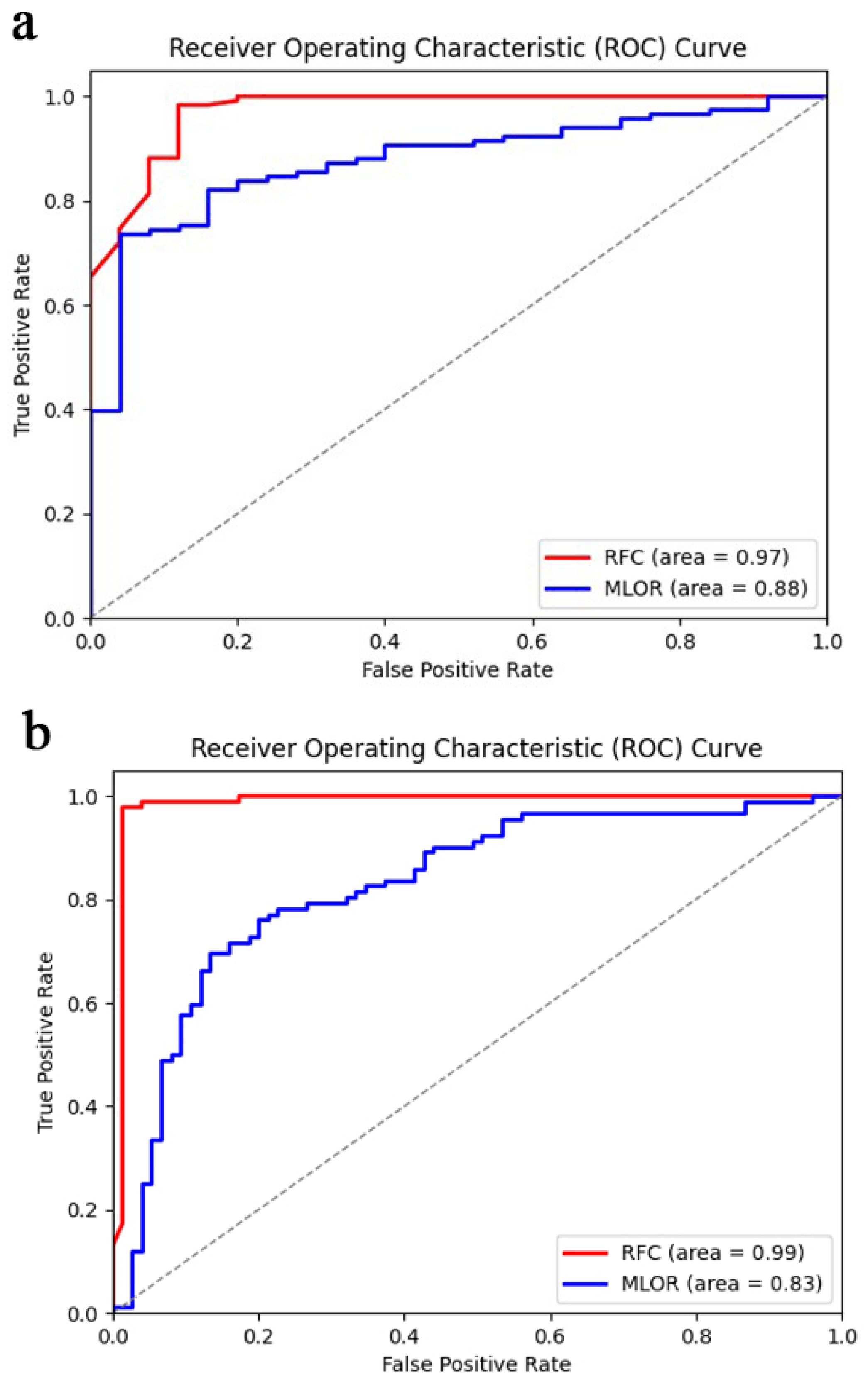
3.2. Performance of Estimation Models

Model validation results (Figure 5 and Figure 6) indicate that the RFR model demonstrates superior performance in estimating arsenic (As) concentrations, capturing 80% and 70% of the spatial variability in the Hetao Basin and Bangladesh, respectively. This performance underscores the RFR model’s high accuracy and robustness, especially in managing the intricacies of complex environmental datasets. The RFR model’s ability to handle non-linear relationships and high-dimensional data attributes significantly to its effectiveness, making it a highly suitable tool for environmental science research.

In contrast, the MLIR model explains only 35% and 32% of the spatial variability in the same regions. This substantial discrepancy highlights the limitations of MLIR in capturing the complex, non-linear interactions that characterize environmental data. The inferior performance of MLIR underscores its inadequacy in contexts where data complexity and dimensionality are paramount.

The findings clearly advocate for the preferential use of sophisticated and flexible regression methods like RFR in environmental studies. The RFR model’s superior handling of non-linearity and high-dimensional datasets makes it a valuable tool for researchers aiming to achieve accurate and reliable predictions. Moreover, the robustness of RFR in diverse geographical settings, as evidenced by its performance in both the Hetao Basin and Bangladesh, further solidifies its applicability and utility in global environmental science endeavors.

In terms of computational efficiency and scalability, while the RFR model offers superior predictive accuracy, it is computationally intensive, particularly with large datasets, due to its ensemble nature and the need for multiple tree evaluations. This can pose challenges in scalability and real-time application. Conversely, MLIR is more computationally efficient and easier to scale given its simpler structure, which involves solving linear equations. Regarding interpretability, MLIR is inherently more interpretable due to its straightforward linear relationships, which facilitate understanding and communication of the influence of each predictor variable. In contrast, the RFR model, despite its high accuracy, suffers from lower interpretability as it functions as a “black box” [36], making it difficult to discern the individual contributions of predictors to the overall model output.

In order to make full use of the advantages of both models, optimization techniques such as hyperparameter tuning, feature selection, and dimensionality reduction can be applied. Furthermore, hybrid approaches can improve predictive accuracy. For instance, combining RFR with MLIR through ensemble methods like stacking or blending can enhance model performance. In such hybrid models, MLIR can provide baseline predictions, while RFR can capture complex patterns and residuals, leading to a more robust and accurate predictive framework.

In conclusion, for environmental studies that necessitate dealing with complex data structures and seeking high predictive accuracy, the random forest regression model stands out as the preferred methodological approach. Future research should prioritize the implementation of such advanced regression techniques to enhance the precision and reliability of environmental assessments and predictions.

3.3. Application of the Binary Classification Models for Groundwater Arsenic Contamination Probability in Hetao Basin and Bangladesh

Based on the aforementioned results from MLIR and RFR, we developed models to predict the probability of high As contamination in groundwater in the Hetao Basin and Bangladesh using RFC and MLOR. The classification results for our training dataset, along with the AUC values, demonstrate strong predictive capabilities. Specifically, the AUC for the RFC model is 0.97 for the Hetao Basin and 0.99 for Bangladesh, significantly outperforming the MLOR model, which has an AUC of 0.88 for the Hetao Basin and 0.83 for Bangladesh (Figure 7a,b). For the training dataset (

Table 3. Classification results for the predictive models in Hetao Basin and Bangladesh.

	Correct Classification	False Positive	False Negative
	Training Dataset
MLOR (Hetao Basin)	82.76%	10.35%	6.90%
MLOR (Bangladesh)	79.41%	17.65%	2.94%
RFC (Hetao Basin)	98.70%	0.88%	0.42%
RFC (Bangladesh)	98.25%	0.75%	1.00%
	Validation Dataset
MLOR (Hetao Basin)	81.60%	17.50%	0.90%
MLOR (Bangladesh)	72.18%	19.55%	8.27%
RFC (Hetao Basin)	82.76%	15.24%	2.00%
RFC (Bangladesh)	91.20%	2.94%	5.88%

Note: The cutoff value is 0.48.

), the MLOR model achieved a correct classification rate of 82.76% for the Hetao Basin, with a false positive rate of 10.35% and a false negative rate of 6.90%. For Bangladesh, the MLOR model had a correct classification rate of 79.41%, a false positive rate of 17.65%, and a false negative rate of 2.94%. In comparison, the RFC model showed significantly higher performance on the training dataset, with a correct classification rate of 98.70% for the Hetao Basin and 98.25% for Bangladesh. The false positive and false negative rates for the RFC model were substantially lower, at 0.88% and 0.42% for the Hetao Basin and 0.75% and 1.00% for Bangladesh, respectively. The classification results of the predictive model for Hetao Basin and Bangladesh are given in Table 3.

In the validation dataset, the MLOR model’s performance decreased slightly, achieving a correct classification rate of 81.60% for the Hetao Basin with a false positive rate of 17.50% and a false negative rate of 0.90%. In Bangladesh, the MLOR model’s correct classification rate dropped to 72.18%, with false positive and false negative rates of 19.55% and 8.27%, respectively. The RFC model maintained a better performance on the validation dataset as well, with a correct classification rate of 82.76% for the Hetao Basin and 91.20% for Bangladesh. The false positive and false negative rates for the RFC model were 15.24% and 2.00% for the Hetao Basin, and 2.94% and 5.88% for Bangladesh, respectively. These observations highlight the RFC model’s enhanced robustness and predictive accuracy. The superior performance of the RFC model in validation datasets underscores its capability to generalize better across different geographic contexts, maintaining lower error rates and higher classification accuracy. This robustness suggests that the RFC model is more effective in adapting to variations in validation data compared to the MLOR model. This improved performance demonstrates the RFC model’s reliability and strong predictive power for identifying high arsenic contamination in groundwater.

3.4. Mechanisms Controlling Geogenic Groundwater as Contamination in Hetao Basin and Bangladesh

According to the results of the RFR and MLIR models, key indicators for the occurrence of geogenic high As groundwater in the Hetao Basin include concentrations of SO₄²⁻, Fe, pH, Cl⁻, Eh, and Ca²⁺, whereas in Bangladesh, the important indicators are SO₄²⁻, Fe, pH, and DOC. Studies have demonstrated that the Holocene strata in the Hetao Basin are generally rich in organic carbon [69]. During the degradation of organic matter (OM), Fe can be utilized as an electron acceptor, leading to the reduction of Fe oxides/oxyhydroxides and the subsequent release of coexisting As [70,71]. The dissolution of Fe oxides is further exacerbated by low redox conditions, which are often indicated by low Eh values. As Fe oxides dissolve, As is released into the groundwater. In addition to dissolution of Fe oxides, competitions between anions and As can contribute to As mobilization in the Hetao Basin. Sulfate (SO₄²⁻) can undergo microbial reduction to sulfide (S²⁻) under anaerobic conditions, which can then react with Fe to form iron sulfide minerals, further releasing As previously adsorbed onto Fe oxides. Chloride (Cl⁻) can also compete with As for adsorption sites, reducing As adsorption and increasing its mobility in groundwater. The positive correlation between As and pH suggests that higher pH levels are often associated with As enrichment in groundwater. Arsenate, the predominant As species in the Hetao Basin’s groundwater, exhibits the greatest adsorption at low pH, with adsorption decreasing as pH increases [72]. This decrease in adsorption at higher pH levels results in higher concentrations of As in the groundwater. Furthermore, under alkaline conditions, Ca²⁺ can co-precipitate with As species to form compounds such as CaH₂AsO₄⁺, CaHAsO₄, and CaAsO₄⁻ [73], which may temporarily reduce As mobility but can dissolve under changing geochemical conditions.

Compared to the Hetao Basin, soil organic carbon content was more pronounced in influencing groundwater As concentration. The aquifer sediments in Bangladesh contain OM and peat, as reported in several studies [74,75]. The degradation of OM within the aquifer generates DOC [76]. Under reducing conditions, higher DOC facilitates the Fe reduction and releases As from younger sediments [77,78]. This process is supported by microbial activity that utilizes DOC as an energy source, leading to the reduction of Fe(III) to Fe(II) and the concomitant release of As adsorbed onto Fe oxides. Furthermore, a negative correlation between As and sulfate ions suggests that As dissolution occurs under reducing conditions. Sulfate reduction can lead to the formation of sulfide, which can react with Fe to form iron sulfides. This process can either sequester As within newly formed minerals or release it from Fe oxide surfaces, depending on the specific geochemical conditions. The presence of DOC further enhances this process by providing the necessary organic substrate for sulfate-reducing bacteria.

These mechanisms illustrate how the interplay of redox conditions, organic matter degradation, and competitive adsorption processes influence the concentration and mobility of As in groundwater in both the Hetao Basin and Bangladesh.

4. Conclusions and Recommendations

This study demonstrates that groundwater As enrichment in both inland basins and floodplains is predominantly influenced by hydro-chemical factors, with geological features such as topography contributing to regional variations. Water-rock interactions are fundamental to the mobilization of As, with specific hydro-chemical and geological data providing valuable indicators for predicting As levels in groundwater. The RFR model was better than MLIR in predicting groundwater As contamination, offering more accurate predictions closely aligned with actual values in both training and validation datasets. Additionally, the RFC model outperformed the MLOR model in predicting high As groundwater probability, capturing nuanced variations and demonstrating higher accuracy. These findings highlight the potential of the random forest approach as a robust tool for predicting global As exposure risks. The practical implications of our findings for environmental management and policy-making are significant. Integrating predictive models like RFR and RFC into existing monitoring frameworks can vastly improve the management and mitigation of arsenic contamination. Predictive models can guide the allocation of resources for monitoring, enabling targeted sampling in high-risk areas and thereby optimizing efforts to mitigate As contamination. Based on the results, the following recommendations have been enlisted below:

• Continual calibration and validation: Regularly calibrate and validate prediction models using diverse datasets to enhance the accuracy and reliability of groundwater As predictions. This iterative process ensures that models remain accurate as new data become available.
• Implement comprehensive monitoring programs: Implement comprehensive monitoring programs that include regular sampling and analysis of hydro-chemical and geological parameters to provide up-to-date data for model inputs. This approach helps in maintaining the accuracy of predictive models and allows for early detection of potential contamination events.
• Strategic management plans: Develop and implement strategic management plans based on predictive model outcomes to mitigate As contamination in high-risk areas. Policies should focus on sustainable groundwater management and remediation efforts tailored to the specific conditions indicated by model predictions.
• Academic research integration: Foster continuous academic research that integrates hydrogeology, geochemistry, and data science to comprehensively address the complex challenge of groundwater As contamination. This multidisciplinary approach can lead to innovative solutions and improvements in prediction models.
• Public health initiatives: Strengthen public health initiatives by disseminating information on As risks and providing resources for safe water alternatives in affected regions. Public awareness and education are crucial for minimizing exposure and protecting health.
• International collaboration: Encourage international collaboration to share knowledge, data, and resources, enhancing the global capacity to effectively predict and manage groundwater As contamination. Collaboration can lead to the development of more robust models and shared strategies for mitigation.

By adopting these recommendations, we can improve the predictive accuracy of groundwater As models and develop effective strategies to safeguard aquifers and protect human health from the adverse effects of As contamination.

Despite the robust findings, there are potential limitations and confounding factors that could influence groundwater As contamination. These include data quality and availability, as the accuracy of predictive models depends on the quality and availability of input data; inconsistent or sparse data, which can reduce the model’s reliability; temporal variations, as groundwater As concentrations can vary seasonally and annually, and so models must account for these temporal variations to provide accurate predictions over time; complex hydrogeological interactions, as interactions between various hydro-chemical and geological factors are complex and not fully understood, and simplifications and assumptions in the models might overlook some critical interactions; and human activities, since agricultural practices, industrial activities, and land use changes can significantly impact groundwater As levels. These anthropogenic factors should be integrated into predictive models to improve their accuracy.

The findings of this study underscore the importance of hydro-chemical factors in influencing groundwater As contamination and highlight the effectiveness of random forest models in predicting As exposure risks. By integrating these predictive models into environmental management frameworks, we can enhance the precision of As contamination predictions and develop effective strategies to safeguard aquifers and protect public health. Adopting the outlined recommendations will improve model accuracy and reliability, foster interdisciplinary research, and promote international collaboration, ultimately leading to better management and mitigation of groundwater As contamination on a global scale.

References

1. Argos, M.; Kalra, T.; Rathouz, P.J.; Chen, Y.; Pierce, B.; Parvez, F.; Islam, T.; Ahmed, A.; Rakibuz-Zaman, M.; Hasan, R.; et al. Arsenic Exposure from Drinking Water, and All-Cause and Chronic-Disease Mortalities in Bangladesh (HEALS): A Prospective Cohort Study. Lancet 2010, 376, 252–258. [Google Scholar] [CrossRef] [PubMed]
2. Chowdhury, U.K.; Biswas, B.K.; Chowdhury, T.R.; Samanta, G.; Mandal, B.K.; Basu, G.C.; Chanda, C.R.; Lodh, D.; Saha, K.C.; Mukherjee, S.K.; et al. Groundwater Arsenic Contamination in Bangladesh and West Bengal, India. Environ. Health Perspect. 2000, 108, 393–397. [Google Scholar] [CrossRef] [PubMed]
3. Karim, M.M. Arsenic in Groundwater and Health Problems in Bangladesh. Water Res. 2000, 34, 304–310. [Google Scholar] [CrossRef]
4. Roberts, L.C.; Hug, S.J.; Dittmar, J.; Voegelin, A.; Saha, G.C.; Ali, M.A.; Badruzzaman, A.B.M.; Kretzschmar, R. Spatial Distribution and Temporal Variability of Arsenic in Irrigated Rice Fields in Bangladesh. 1. Irrigation Water. Environ. Sci. Technol. 2007, 41, 5960–5966. [Google Scholar] [CrossRef] [PubMed]
5. Concha, G.; Nermell, B.; Vahter, M. Spatial and Temporal Variations in Arsenic Exposure via Drinking-Water in Northern Argentina. J. Health Popul. Nutr. 2006, 24, 317–326. [Google Scholar] [PubMed]
6. Dittmar, J.; Voegelin, A.; Roberts, L.C.; Hug, S.J.; Saha, G.C.; Ali, M.A.; Badruzzaman, A.B.M.; Kretzschmar, R. Spatial Distribution and Temporal Variability of Arsenic in Irrigated Rice Fields in Bangladesh. 2. Paddy Soil. Environ. Sci. Technol. 2007, 41, 5967–5972. [Google Scholar] [CrossRef] [PubMed]
7. Mahimairaja, S.; Bolan, N.S.; Adriano, D.C.; Robinson, B. Arsenic Contamination and Its Risk Management in Complex Environmental Settings. Adv. Agron. 2005, 86, 1–82. [Google Scholar]
8. Ayotte, J.D.; Nolan, B.T.; Nuckols, J.R.; Cantor, K.P.; Robinson, G.R.; Baris, D.; Hayes, L.; Karagas, M.; Bress, W.; Silverman, D.T.; et al. Modeling the Probability of Arsenic in Groundwater in New England as a Tool for Exposure Assessment. Environ. Sci. Technol. 2006, 40, 3578–3585. [Google Scholar] [CrossRef] [PubMed]
9. Nordstrom, D.K. Arsenic in the Geosphere Meets the Anthroposphere. In Proceedings of the Understanding the Geological and Medical Interface of Arsenic, As 2012—4th International Congress: Arsenic in the Environment, Cairns, Australia, 22–27 July 2012. [Google Scholar]
10. Smedley, P.; Zhang, M.; Zhang, G.; Luo, Z. Mobilisation of Arsenic and Other Trace Elements in Fluviolacustrine Aquifers of the Huhhot Basin, Inner Mongolia. Appl. Geochem. 2003, 18, 1453–1477. [Google Scholar] [CrossRef]
11. Wang, Y.; Pi, K.; Fendorf, S.; Deng, Y.; Xie, X. Sedimentogenesis and Hydrobiogeochemistry of High Arsenic Late Pleistocene-Holocene Aquifer Systems. Earth-Sci. Rev. 2019, 189, 79–98. [Google Scholar] [CrossRef]
12. Harvey, C.F.; Swartz, C.H.; Badruzzaman, A.B.M.; Keon-Blute, N.; Yu, W.; Ali, M.A.; Jay, J.; Beckie, R.; Niedan, V.; Brabander, D.; et al. Arsenic Mobility and Groundwater Extraction in Bangladesh. Science 2002, 298, 1602–1606. [Google Scholar] [CrossRef] [PubMed]
13. van Geen, A.; Bostick, B.C.; Trang, P.T.K.; Lan, V.M.; Mai, N.-N.; Manh, P.D.; Viet, P.H.; Radloff, K.; Aziz, Z.; Mey, J.L.; et al. Retardation of Arsenic Transport through a Pleistocene Aquifer. Nature 2013, 501, 204–207. [Google Scholar] [CrossRef]
14. Masscheleyn, P.H.; Delaune, R.D.; Patrick, W.H. Effect of Redox Potential and pH on Arsenic Speciation and Solubility in a Contaminated Soil. Environ. Sci. Technol. 1991, 25, 1414–1419. [Google Scholar] [CrossRef]
15. Guo, H.; Liu, C.; Lu, H.; Wanty, R.B.; Wang, J.; Zhou, Y. Pathways of Coupled Arsenic and Iron Cycling in High Arsenic Groundwater of the Hetao Basin, Inner Mongolia, China: An Iron Isotope Approach. Geochim. Cosmochim. Acta 2013, 112, 130–145. [Google Scholar] [CrossRef]
16. Luo, T.; Hu, S.; Cui, J.; Tian, H.; Jing, C. Comparison of Arsenic Geochemical Evolution in the Datong Basin (Shanxi) and Hetao Basin (Inner Mongolia), China. Appl. Geochem. 2012, 27, 2315–2323. [Google Scholar] [CrossRef]
17. Zhang, H.; Ma, D.; Hu, X. Arsenic Pollution in Groundwater from Hetao Area, China. Environ. Geol. 2002, 41, 638–643. [Google Scholar] [CrossRef]
18. Zheng, Y.; Stute, M.; van Geen, A.; Gavrieli, I.; Dhar, R.; Simpson, H.; Schlosser, P.; Ahmed, K. Redox Control of Arsenic Mobilization in Bangladesh Groundwater. Appl. Geochem. 2004, 19, 201–214. [Google Scholar] [CrossRef]
19. Zheng, Y.; van Geen, A.; Stute, M.; Dhar, R.; Mo, Z.; Cheng, Z.; Horneman, A.; Gavrieli, I.; Simpson, H.; Versteeg, R.; et al. Geochemical and Hydrogeological Contrasts between Shallow and Deeper Aquifers in Two Villages of Araihazar, Bangladesh: Implications for Deeper Aquifers as Drinking Water Sources. Geochim. Cosmochim. Acta 2005, 69, 5203–5218. [Google Scholar] [CrossRef]
20. Buschmann, J.; Berg, M.; Stengel, C.; Sampson, M.L. Arsenic and Manganese Contamination of Drinking Water Resources in Cambodia: Coincidence of Risk Areas with Low Relief Topography. Environ. Sci. Technol. 2007, 41, 2146–2152. [Google Scholar] [CrossRef] [PubMed]
21. Anawar, H.M.; Akai, J.; Komaki, K.; Terao, H.; Yoshioka, T.; Ishizuka, T.; Safiullah, S.; Kato, K. Geochemical Occurrence of Arsenic in Groundwater of Bangladesh: Sources and Mobilization Processes. J. Geochem. Explor. 2003, 77, 109–131. [Google Scholar] [CrossRef]
22. Baig, J.A.; Kazi, T.G.; Arain, M.B.; Afridi, H.I.; Kandhro, G.A.; Sarfraz, R.A.; Jamal, M.K.; Shah, A.Q. Evaluation of Arsenic and Other Physico-Chemical Parameters of Surface and Ground Water of Jamshoro, Pakistan. J. Hazard. Mater. 2009, 166, 662–669. [Google Scholar] [CrossRef] [PubMed]
23. Podgorski, J.E.; Eqani, S.A.M.A.S.; Khanam, T.; Ullah, R.; Shen, H.; Berg, M. Extensive Arsenic Contamination in High-pH Unconfined Aquifers in the Indus Valley. Sci. Adv. 2017, 3, e1700935. [Google Scholar] [CrossRef] [PubMed]
24. Rodríguez-lado, L.; Sun, G.; Berg, M.; Zhang, Q.; Xue, H.; Zheng, Q.; Johnson, C.A. Groundwater Arsenic Contamination throughout China. Science 2013, 341, 866–868. [Google Scholar] [CrossRef] [PubMed]
25. Chakraborty, M.; Sarkar, S.; Mukherjee, A.; Shamsudduha, M.; Ahmed, K.M.; Bhattacharya, A.; Mitra, A. Modeling Regional-Scale Groundwater Arsenic Hazard in the Transboundary Ganges River Delta, India and Bangladesh: Infusing Physically-Based Model with Machine Learning. Sci. Total Environ. 2020, 748, 141107. [Google Scholar] [CrossRef] [PubMed]
26. Tan, K.; Ye, Y.; Cao, Q.; Du, P.; Dong, J. Estimation of Arsenic Contamination in Reclaimed Agricultural Soils Using Reflectance Spectroscopy and ANFIS Model. IEEE J. Sel. Top. Appl. Earth Obs. Remote Sens. 2014, 7, 2540–2546. [Google Scholar] [CrossRef]
27. Podgorski, J.; Araya, D.; Berg, M. Geogenic Manganese and Iron in Groundwater of Southeast Asia and Bangladesh—Machine Learning Spatial Prediction Modeling and Comparison with Arsenic. Sci. Total Environ. 2022, 833, 155131. [Google Scholar] [CrossRef] [PubMed]
28. Cho, K.H.; Sthiannopkao, S.; Pachepsky, Y.A.; Kim, K.-W.; Kim, J.H. Prediction of Contamination Potential of Groundwater Arsenic in Cambodia, Laos, and Thailand Using Artificial Neural Network. Water Res. 2011, 45, 5535–5544. [Google Scholar] [CrossRef] [PubMed]
29. Charulatha, G.; Srinivasalu, S.; Maheswari, O.U.; Venugopal, T.; Giridharan, L. Evaluation of Ground Water Quality Contaminants Using Linear Regression and Artificial Neural Network Models. Arab. J. Geosci. 2017, 10, 128. [Google Scholar] [CrossRef]
30. Sayegh, A.S.; Munir, S.; Habeebullah, T.M. Comparing the Performance of Statistical Models for Predicting PM10 Concentrations. Aerosol Air Qual. Res. 2014, 14, 653–665. [Google Scholar] [CrossRef]
31. Haggerty, R.; Sun, J.; Yu, H.; Li, Y. Application of Machine Learning in Groundwater Quality Modeling—A Comprehensive Review. Water Res. 2023, 233, 119745. [Google Scholar] [CrossRef] [PubMed]
32. Ouedraogo, I.; Defourny, P.; Vanclooster, M. Application of Random Forest Regression and Comparison of Its Performance to Multiple Linear Regression in Modeling Groundwater Nitrate Concentration at the African Continent Scale. Hydrogeol. J. 2019, 27, 1081–1098. [Google Scholar] [CrossRef]
33. Tesoriero, A.J.; Gronberg, J.A.; Juckem, P.F.; Miller, M.P.; Austin, B.P. Predicting Redox-Sensitive Contaminant Concentrations in Groundwater Using Random Forest Classification. Water Resour. Res. 2017, 53, 7316–7331. [Google Scholar] [CrossRef]
34. Akakuru, O.C.; Akaolisa, C.C.Z.; Aigbadon, G.O.; Eyankware, M.O.; Opara, A.I.; Obasi, P.N.; Ofoh, I.J.; Njoku, A.O.; Akudinobi, B.E.B. Integrating Machine Learning and Multi-Linear Regression Modeling Approaches in Groundwater Quality Assessment around Obosi, Se Nigeria. Environ. Dev. Sustain. 2023, 25, 14567–14606. [Google Scholar] [CrossRef]
35. Saghebian, S.M.; Sattari, M.T.; Mirabbasi, R.; Pal, M. Ground Water Quality Classification by Decision Tree Method in Ardebil Region, Iran. Arab. J. Geosci. 2014, 7, 4767–4777. [Google Scholar] [CrossRef]
36. Biau, G.; Scornet, E. A Random Forest Guided Tour. Test 2016, 25, 197–227. [Google Scholar] [CrossRef]
37. Liaw, A.; Wiener, M. Classification and Regression by RandomForest. R News 2002, 2, 18–22. [Google Scholar]
38. Tan, Z.; Yang, Q.; Zheng, Y. Machine Learning Models of Groundwater Arsenic Spatial Distribution in Bangladesh: Influence of Holocene Sediment Depositional History. Environ. Sci. Technol. 2020, 54, 9454–9463. [Google Scholar] [CrossRef] [PubMed]
39. Bindal, S.; Singh, C.K. Predicting Groundwater Arsenic Contamination: Regions at Risk in Highest Populated State of India. Water Res. 2019, 159, 65–76. [Google Scholar] [CrossRef]
40. Feng, L.-X.; Brown, R.W.; Han, B.-F.; Wang, Z.-Z.; Łuszczak, K.; Liu, B.; Zhang, Z.-C.; Ji, J.-Q. Thrusting and Exhumation of the Southern Mongolian Plateau: Joint Thermochronological Constraints from the Langshan Mountains, Western Inner Mongolia, China. J. Asian Earth Sci. 2017, 144, 287–302. [Google Scholar] [CrossRef]
41. He, J.; Ma, T.; Deng, Y.; Yang, H.; Wang, Y. Environmental Geochemistry of High Arsenic Groundwater at Western Hetao Plain, Inner Mongolia. Front. Earth Sci. China 2009, 3, 63–72. [Google Scholar] [CrossRef]
42. Guo, H.; Yang, S.; Tang, X.; Li, Y.; Shen, Z. Groundwater Geochemistry and Its Implications for Arsenic Mobilization in Shallow Aquifers of the Hetao Basin, Inner Mongolia. Sci. Total Environ. 2008, 393, 131–144. [Google Scholar] [CrossRef] [PubMed]
43. Deng, Y.; Wang, Y.; Ma, T. Isotope and Minor Element Geochemistry of High Arsenic Groundwater from Hangjinhouqi, the Hetao Plain, Inner Mongolia. Appl. Geochem. 2009, 24, 587–599. [Google Scholar] [CrossRef]
44. Gao, Z.; Weng, H.; Guo, H. Unraveling Influences of Nitrogen Cycling on Arsenic Enrichment in Groundwater from the Hetao Basin Using Geochemical and Multi-Isotopic Approaches. J. Hydrol. 2021, 595, 125981. [Google Scholar] [CrossRef]
45. Goodbred, S.L.; Kuehl, S.A. The Significance of Large Sediment Supply, Active Tectonism, and Eustasy on Margin Sequence Development: Late Quaternary Stratigraphy and Evolution of the Ganges–Brahmaputra Delta. Sediment. Geol. 2000, 133, 227–248. [Google Scholar] [CrossRef]
46. Karim, M.M.; Safiuddin, M. Arsenic Contamination of Groundwater in Bangladesh; British Geological Survey Technical Report WC/00/19; British Geological Survey: Nottingham, UK, 2001; Volume 4, pp. 162–165. [Google Scholar]
47. Acharyya, S.K.; Lahiri, S.; Raymahashay, B.C.; Bhowmik, A. Arsenic Toxicity of Groundwater in Parts of the Bengal Basin in India and Bangladesh: The Role of Quaternary Stratigraphy and Holocene Sea-Level Fluctuation. Environ. Geol. 2000, 39, 1127–1137. [Google Scholar] [CrossRef]
48. Huang, G.; Song, J.; Han, D.; Liu, R.; Liu, C.; Hou, Q. Assessing Natural Background Levels of Geogenic Contaminants in Groundwater of an Urbanized Delta through Removal of Groundwaters Impacted by Anthropogenic Inputs: New Insights into Driving Factors. Sci. Total Environ. 2023, 857, 159527. [Google Scholar] [CrossRef] [PubMed]
49. Rodríguez, R.; Ramos, J.; Armienta, A. Groundwater Arsenic Variations: The Role of Local Geology and Rainfall. Appl. Geochem. 2004, 19, 245–250. [Google Scholar] [CrossRef]
50. Huang, G.; Zhang, M.; Liu, C.; Li, L.; Chen, Z. Heavy Metal(loid)s and Organic Contaminants in Groundwater in the Pearl River Delta That Has Undergone Three Decades of Urbanization and Industrialization: Distributions, Sources, and Driving Forces. Sci. Total Environ. 2018, 635, 913–925. [Google Scholar] [CrossRef] [PubMed]
51. Huang, G.; Chen, Z.; Liu, F.; Sun, J.; Wang, J. Impact of Human Activity and Natural Processes on Groundwater Arsenic in an Urbanized Area (South China) Using Multivariate Statistical Techniques. Environ. Sci. Pollut. Res. 2014, 21, 13043–13054. [Google Scholar] [CrossRef] [PubMed]
52. Pukelsheim, F. The Three Sigma Rule. Am. Stat. 1994, 48, 88–91. [Google Scholar] [CrossRef]
53. Ahmad, S.; Ahmad, I.; Umar, R.; Farooq, S.H. Spatio-Temporal Variation and Health Risk Associated with Trace Element Concentrations in Groundwater of Mathura City Using Modified Indexing Approach. Arab. J. Geosci. 2022, 15, 318. [Google Scholar] [CrossRef]
54. Li, X.; Ge, J.; Liu, Z.; Yang, S.; Wang, L.; Liu, Y. Estimating the Methane Flux of the Dajiuhu Subalpine Peatland Using Machine Learning Algorithms and the Maximal Information Coefficient Technique. Sci. Total Environ. 2024, 916, 170241. [Google Scholar] [CrossRef] [PubMed]
55. Rodriguez-Galiano, V.; Mendes, M.P.; Garcia-Soldado, M.J.; Chica-Olmo, M.; Ribeiro, L. Predictive Modeling of Groundwater Nitrate Pollution Using Random Forest and Multisource Variables Related to Intrinsic and Specific Vulnerability: A Case Study in an Agricultural Setting (Southern Spain). Sci. Total Environ. 2014, 476–477, 189–206. [Google Scholar] [CrossRef] [PubMed]
56. Khosravi, K.; Mao, L.; Kisi, O.; Yaseen, Z.M.; Shahid, S. Quantifying Hourly Suspended Sediment Load Using Data Mining Models: Case Study of a Glacierized Andean Catchment in Chile. J. Hydrol. 2018, 567, 165–179. [Google Scholar] [CrossRef]
57. Sharafati, A.; Khosravi, K.; Khosravinia, P.; Ahmed, K.; Salman, S.A.; Yaseen, Z.M.; Shahid, S. The Potential of Novel Data Mining Models for Global Solar Radiation Prediction. Int. J. Environ. Sci. Technol. 2019, 16, 7147–7164. [Google Scholar] [CrossRef]
58. Jin, Z.; Shang, J.; Zhu, Q.; Ling, C.; Xie, W.; Qiang, B. RFRSF: Employee Turnover Prediction Based on Random Forests and Survival Analysis. In Web Information Systems Engineering—WISE 2020; Lecture Notes in Computer Science; Springer: Cham, Swizerland, 2020; Volume 12343, pp. 503–515. [Google Scholar] [CrossRef]
59. Guo, W.; Gao, Z.; Guo, H.; Cao, W. Hydrogeochemical and Sediment Parameters Improve Predication Accuracy of Arsenic-Prone Groundwater in Random Forest Machine-Learning Models. Sci. Total Environ. 2023, 897, 165511. [Google Scholar] [CrossRef] [PubMed]
60. Zhang, Q.; Rodríguez-Lado, L.; Johnson, C.A.; Xue, H.; Shi, J.; Zheng, Q.; Sun, G. Predicting the Risk of Arsenic Contaminated Groundwater in Shanxi Province, Northern China. Environ. Pollut. 2012, 165, 118–123. [Google Scholar] [CrossRef] [PubMed]
61. Raschka, S. Python Machine Learning, 1st ed.; Equation Reference; Packt Publishing: Birmingham, UK, 2015; Volume 2015, pp. 1–71. [Google Scholar]
62. Chen, W.; Tsangaratos, P.; Ilia, I.; Duan, Z.; Chen, X. Groundwater Spring Potential Mapping Using Population-Based Evolutionary Algorithms and Data Mining Methods. Sci. Total Environ. 2019, 684, 31–49. [Google Scholar] [CrossRef] [PubMed]
63. Bellu, A.; Fernandes, L.F.S.; Cortes, R.M.V.; Pacheco, F.A.L. A Framework Model for the Dimensioning and Allocation of a Detention Basin System: The Case of a Flood-Prone Mountainous Watershed. J. Hydrol. 2016, 533, 567–580. [Google Scholar] [CrossRef]
64. Wang, H.; Eiche, E.; Guo, H.; Norra, S. Impact of Sedimentation History for As Distribution in Late Pleistocene-Holocene Sediments in the Hetao Basin, China. J. Soils Sediments 2020, 20, 4070–4082. [Google Scholar] [CrossRef]
65. Guo, H.; Zhang, B.; Li, Y.; Berner, Z.; Tang, X.; Norra, S.; Stüben, D. Hydrogeological and Biogeochemical Constrains of Arsenic Mobilization in Shallow Aquifers from the Hetao Basin, Inner Mongolia. Environ. Pollut. 2011, 159, 876–883. [Google Scholar] [CrossRef] [PubMed]
66. Bauer, M.; Blodau, C. Mobilization of Arsenic by Dissolved Organic Matter from Iron Oxides, Soils and Sediments. Sci. Total Environ. 2006, 354, 179–190. [Google Scholar] [CrossRef] [PubMed]
67. Guo, H.; Li, X.; Xiu, W.; He, W.; Cao, Y.; Zhang, D.; Wang, A. Controls of Organic Matter Bioreactivity on Arsenic Mobility in Shallow Aquifers of the Hetao Basin, P.R. China. J. Hydrol. 2019, 571, 448–459. [Google Scholar] [CrossRef]
68. Khalid, S.; Shahid, M.; Niazi, N.K.; Rafiq, M.; Bakhat, H.F.; Imran, M.; Abbas, T.; Bibi, I.; Dumat, C. Arsenic Behaviour in Soil-Plant System: Biogeochemical Reactions and Chemical Speciation Influences. In Enhancing Cleanup of Environmental Pollutants; Springer: Cham, Switzerland, 2017; Volume 2. [Google Scholar]
69. Deng, Y.; Wang, Y.; Ma, T.; Gan, Y. Speciation and Enrichment of Arsenic in Strongly Reducing Shallow Aquifers at Western Hetao Plain, Northern China. Environ. Geol. 2009, 56, 1467–1477. [Google Scholar] [CrossRef]
70. Postma, D.; Larsen, F.; Thai, N.T.; Trang, P.T.K.; Jakobsen, R.; Nhan, P.Q.; Long, T.V.; Viet, P.H.; Murray, A.S. Groundwater Arsenic Concentrations in Vietnam Controlled by Sediment Age. Nat. Geosci. 2012, 5, 656–661. [Google Scholar] [CrossRef]
71. Rowland, H.A.L.; Pederick, R.L.; Polya, D.A.; Pancost, R.D.; Van Dongen, B.E.; Gault, A.G.; Vaughan, D.J.; Bryant, C.; Anderson, B.; Lloyd, J.R. The Control of Organic Matter on Microbially Mediated Iron Reduction and Arsenic Release in Shallow Alluvial Aquifers, Cambodia. Geobiology 2007, 5, 281–292. [Google Scholar] [CrossRef]
72. Stollenwerk, K.G. Geochemical Processes Controlling Transport of Arsenic in Groundwater: A Review of Adsorption. In Arsenic in Ground Water; Springer: Boston, MA, USA, 2005. [Google Scholar]
73. Hafeznezami, S.; Zimmer-Faust, A.G.; Jun, D.; Rugh, M.B.; Haro, H.L.; Park, A.; Suh, J.; Najm, T.; Reynolds, M.D.; Davis, J.A.; et al. Remediation of Groundwater Contaminated with Arsenic through Enhanced Natural Attenuation: Batch and Column Studies. Water Res. 2017, 122, 545–556. [Google Scholar] [CrossRef]
74. Nickson, R.T.; McArthur, J.M.; Ravenscroft, P.; Burgess, W.G.; Ahmed, K.M. Mechanism of Arsenic Release to Groundwater, Bangladesh and West Bengal. Appl. Geochem. 2000, 15, 403–413. [Google Scholar] [CrossRef]
75. McArthur, J.M.; Ravenscroft, P.; Safiulla, S.; Thirlwall, M.F. Arsenic in Groundwater: Testing pollution Mechanisms for Sedimentary Aquifers in Bangladesh. Water Resour. Res. 2001, 37, 109–117. [Google Scholar] [CrossRef]
76. Aiken, G.; Kuniansky, E.L. U.S. Geological Survey Artificial Recharge Workshop Proceedings, April 2-4, 2002, Sacramento, California; U.S. Geological Survey: Reston, VA, USA, 2002; pp. 47–50. [Google Scholar]
77. Bhattacharya, P.; Welch, A.H.; Ahmed, K.M.; Jacks, G.; Naidu, R. Arsenic in Groundwater of Sedimentary Aquifers. Appl. Geochem. 2004, 19, 163–167. [Google Scholar] [CrossRef]
78. Akai, J.; Izumi, K.; Fukuhara, H.; Masuda, H.; Nakano, S.; Yoshimura, T.; Ohfuji, H.; Anawar, H.M.; Akai, K. Mineralogical and Geomicrobiological Investigations on Groundwater Arsenic Enrichment in Bangladesh. Appl. Geochem. 2004, 19, 215–230. [Google Scholar] [CrossRef]
79. Cao, W.; Guo, H.; Zhang, Y.; Ma, R.; Li, Y.; Dong, Q.; Li, Y.; Zhao, R. Controls of Paleochannels on Groundwater Arsenic Distribution in Shallow Aquifers of Alluvial Plain in the Hetao Basin, China. Sci. Total Environ. 2018, 613–614, 958–968. [Google Scholar] [CrossRef] [PubMed]
Figure 2. Spatial distribution of groundwater arsenic concentrations in Bangladesh (data from [48]).
Water 16 02291 g002
Figure 3. Flow diagram of methodologies adopted for this study.
Water 16 02291 g003
Figure 4. Graphical presentation of Pearson’s Correlation Coefficient. (a): Hetao Basin; (b): Bangladesh. Abbreviations: OCD: organic carbon density; CC: clay content; SOC: soil organic carbon; BD: bulk density; SC: silt content; CEC: cation exchange capacity; DOC: dissolved organic carbon; AsTot: total arsenic.
Water 16 02291 g004
Figure 5. Relationship between predicted and measured As contamination for MLIR model. (a): Training data for Hetao Basin; (b): Training data for Bangladesh; (c): Validation data for Hetao Basin; (d): Validation data for Bangladesh.
Water 16 02291 g005
Figure 6. Relationship between predicted and measured As contamination for RFR model. (a): Training data for Hetao Basin; (b): Training data for Bangladesh; (c): Validation data for Hetao Basin; (d): Validation data for Bangladesh.
Water 16 02291 g006
Figure 7. (a) AUC-ROC of adopted models in Hetao Basin. (b) AUC-ROC of adopted models in Bangladesh.
Water 16 02291 g007