Effects of Fallen Posidonia Oceanica Seagrass Leaves on Wave Energy at Sandy Beaches

Abstract

Posidonia Oceanica (PO) is an endemic marine plant in the Mediterranean Sea. In an experimental study conducted in the Eastern Mediterranean, the effects of natural PO leaves on reducing the height of incident waves impacting a beach were measured. The transmission coefficient (K_t) was found to vary between 0.73 and 0.94, which is equivalent to a wave height decay of 6–27%. The results show that in their natural environment, free-floating dead PO leaves dissipate incoming wave energy and have the capacity to protect beaches against erosion. Further analysis in separate frequency bands showed that waves with periods between 4.5–6.2 s were more sensitive to PO leaves in terms of energy dissipation. The transmission coefficient for medium-period waves, calculated using the medium-frequency part of the wave spectrum, delivered a maximum transmission coefficient of 0.5, corresponding to a 50% decay in wave height due to PO leaves.

1. Introduction

To reduce incoming wave energy along sandy shores, different solutions have been developed, including hard and soft structures. Hard structures can be groins, breakwaters, revetments, and seawalls, which are mainly types of barriers to either reduce the wave energy or trap the sediment in the nearshore. On the other hand, owing to their environmental benefits, nature-based solutions, such as vegetation on the sea bottom, may supplement or even replace conventional erosion protection techniques. In this study, our focus was the wave energy dissipation capacity of sunken or floating leaves of dead seagrass (Posidonia Oceanica) in the nearshore (Figure 1). Posidonia Oceanica (PO) is an endemic marine plant in the Mediterranean Sea, covering an area of 50.000 km² [1], which corresponds to 25% of the basin shallower than 40 m [2]. Along the Mediterranean coast, large meadows of PO are observed where new leaves can bloom all year round. In autumn, the dead leaves fall off the rhizomes and accumulate inside the meadows. Autumn and winter storms drive the fallen PO leaves away from the meadows to other ecosystems [3]. Most of the time, they end up washing ashore, where they form natural banquettes on the beach if not manually removed.

In one of the earliest experimental studies on the effects of sea vegetation on beach profiles, Price et al. (1968) used polypropylene stems fixed at the bottom of a flume to imitate seaweed. They found that fixed stems reversed erosion and accumulated sand by reducing incoming wave height [4]. In subsequent years, theoretical models have been developed to predict wave attenuation induced by sea vegetation. Dalrymple et al. (1984) [5] developed a mathematical model for wave attenuation based on the drag caused by vegetation blades. They modeled the vegetation as rigid cylinders and ignored the relative motion between the blades and the water particles. A Morrison-type drag force was vertically integrated along the stem height to calculate the drag and the energy dissipation per unit area of meadow [5]. As an alternative to Dalrymple et al.’s (1984) [5] hyperbolic decay function, Kobayashi et al. (1993) [6] found that wave height exponentially decayed with distance as waves propagated inside a vegetation field [6]. Mendez and Losada (2004) [7] extended Dalrymple et al.’s (1984) [5] derivation and derived wave dissipation from vegetation on a sloping beach using random waves [7]. Dalrymple et al.’s (1983) [5] and Kobayashi et al.’s (1993) [6] theoretical models argue that the wave height decay induced by sea vegetation is controlled by the drag coefficient of a single stem, whereas Mendez and Losada (2004) [7] defined a bulk drag coefficient, which represents a single value for the entire meadow.

The bulk drag coefficient is used in wave and flow equations to eliminate the sheltering effect of stems on each other. Different dimensionless parameters, including the Reynolds number (Re) [8,9,10], Cauchy number (Ca) [11], and Kauleguen Carpenter number (KC) [12,13], are claimed to have strong correlations with the bulk drag coefficient. Luhar et al. (2017) considered a rigid cylinder with a reduced “effective blade length” that overcame the inconsistency between the theoretical and measured drag coefficient due to the relative motion and sheltering effects [11]. The bulk drag coefficient (C_D) calculation contains calibration parameters that need to be identified through measurements. These parameters are identified by flume tests and by imitating the vegetation. The main drawbacks of such methods are the similarity problem when imitating vegetation and the scale effects. Fonseca and Calahan (1992) [14] and Hendricks et al. (2008) [15] used live vegetation in their flume tests, while others have used different materials to imitate vegetation [14,15]. For instance, Peruzzo et al. (2018) [12] used silicone imitations to represent Spartina maritima in their wave flume [12]. A very-low-melt propylene heterophasic copolymer [13], nickel–chrome strips [16], and wood dowels have been used to represent rigid vegetation, and polyethylene foam has been used to represent flexible vegetation [17].

Almost all of the existing literature focuses on vegetation fixed to the sea bottom by roots and classifies it by its rigidity, stem density per unit area, length, width, and diameter, and its emergence or submergence (submergence ratio, or depth, in the case of submergence). Except for a few field tests [10,18], most tests have been performed using imitated vegetation in a wave flume, which does not represent the actual conditions in nature. In addition, vegetation parameters, which are taken as constant in flume tests, actually change in nature continuously throughout the year, depending on their metabolism. In particular, Posidonia Oceanica seagrass has a life cycle similar to that of terrestrial plants (i.e., they photosynthesize, flower, and defoliate). Its stem density is the lowest during the winter period [19], when the sea is in its most energetic state in terms of wave energy. However, once it defoliates, tons of dead leaves become loose and are transported until they are deposited at the shoreline or degraded within the sea. Therefore, the aim of the present study was to investigate the wave attenuation capacity of defoliated Posidonia Oceanica leaves in their natural environment. Dead leaves can be suspended or sink to the sea bottom depending on their density, which varies between 800 and 1020 kg/m³ [20]. Although they may contribute to wave attenuation in different forms or stages, i.e., while they are in a meadow or after they leave, our interest is in the phase during which the leaves are being transported in the nearshore toward the beach along low-energy coasts.

Since these natural materials exist in the nearshore and surf zone throughout the year, their impact on waves is worth investigating as they are part of natural nearshore processes along many low-energy coasts around the world. To the best of the authors’ knowledge, there have been no field measurements conducted in nature to prove the theoretically known wave dissipation capacity of PO leaves and to experimentally quantify wave energy dissipation with real vegetation and real waves. The present study aims to fill this gap in the literature.

2. Study Area

Field experiments were conducted at Fugla Bay, a headland beach on the Mediterranean Coast of Turkey located between two touristic cities, Antalya and Alanya (Figure 2). The bay has a 1.7 km long sandy beach facing south–west. The area is rich with Posidonia Oceanica (PO) meadows, as 40% of the seabed is covered with PO reefs and bedrock outcrops. The rest of the seabed is a sandy bottom, with an average slope of 1/30.

3. Measurement Method and Site Setup

Field measurements were conducted in April 2023, a time of year when PO leaves are washed ashore. Although defoliation starts as early as in autumn, it normally takes a few storms until all the leaves are accumulated at the shore.

Our aim was to measure the wave heights at three different locations perpendicular to the shore. These were (a) deep water to measure the incident wave characteristics, (b) shallow water before the waves had passed the PO-covered area, and (c) shallow water after the waves had passed the PO-covered area. An acoustic doppler current profiler (ADCP- 1 MHz) and two pressure gauges (PG1 and PG2) were deployed in a row in the direction normal to the shore. The deployment plan and a schematic cross-section of the test setup are shown in Figure 2 and Figure 3, respectively.

As PO leaves move randomly in nature, it was impossible to place the measurement devices in the path of the PO motion before they started moving. Therefore, it was planned to perform the tests under “semi-controlled” conditions, i.e., the PO leaves were trapped in a zone and subjected to real sea waves and bathymetry. The steps of testing are provided below:

STEP 1: The test location was identified as a band normal to the shore where the seabed had the typical slope of 1/30 and a form without any irregularities.

STEP 2: PO leaves that were washed ashore along the same beach were transported to the test site via land transport.

STEP 3: Measurement devices were deployed at the seabed at pre-identified locations.

STEP 4: A fishnet was installed in the cross-shore direction to keep the PO leaves within the testing area.

STEP 5: The PO leaves were manually transported to the testing area in a canoe and released into the water.

The ADCP sampling rates were set to 2 Hz for the pressure measurement and 4 Hz for acoustic surface tracking (AST). The ADCP was operated in bursts of 17 min of continuous recording and 13 min in sleeping mode. Each data burst contained 2048 items of pressure data and 4096 items of AST data. The two custom-made pressure gauges (PG1 and PG2) recorded continuously at 4 Hz without a sleeping mode and with a built-in capacity of 1.2 million records (83 h of data). The device locations are provided in

Table 1. Measurement device locations.

Station ID	Northing (m)	Easting (m)	Device Installed
St 1	390,332.749	4,053,887.423	Acoustic doppler current profiler (ADCP)
St 2	390,426.312	4,053,866.927	Pressure gauge 1 (PG1)
St 3	390,440.026	4,053,864.256	Pressure gauge 2 (PG2)

. The ADCP position under water and a general image of the site can be seen in Figure 4. Prior to their deployment, calibration of each of the devices was carried out at the Boğaziçi University Coastal Engineering Laboratory, Istanbul, Turkey.

Conductivity, salinity, and density measurements of the seawater were performed with an oceanographic measurement device. The average conductivity of the site at the time of the test was 50.1 ms/cm. The salinity and density were measured as 39.09 PSU and 1028.4 kg/m³, respectively. The density measurements were carried out in the laboratory on the samples collected from the site. The pycnometer results indicate a 0.999 kg/m³ density of the PO leaves, which is a lower density than that of seawater. However, once they were dumped into the test location, most of the leaves sank to the bottom due to sand particles adhering to them, which made them heavier than the seawater.

3.1. Bathymetry

Prior to the gauge installation, bathymetric measurements were conducted at the test site. The bottom slope was measured as 1/30. The bathymetric contours of the bay and the bottom profile along the test site are shown in Figure 5.

PO leaves that had washed ashore were collected from the beach and brought to the measurement site by truck. The PO leaves were then loaded into a canoe, carried to the target location, and gradually released into the sea (Figure 6).

As shown in Figure 4b, the PO leaves were released between the two pressure gauges (PG1 and PG2) continuously for four hours at a constant pace until the entire amount of 27 m³ of PO leaves was used. Some of the PO leaves washed ashore during the testing, and some of them escaped the testing zone. The PO leaves piled up between PG1 and PG2, reaching a maximum height of 30 cm at the sea bottom. As shown in Figure 7 at the end of the measurement, the PO leaves were distributed both in the longshore and cross-shore directions. The measurements were continued for several hours after terminating the PO release, so that the remaining PO leaves between PG1 and PG2 were reduced to a minimum and did not affect the wave parameters any further. The findings on how the leaves interacted with the incoming waves are detailed in Section 4.

3.2. Data Analysis

In addition to the underwater electronic wave recorders, aerial drone images were used to track the PO motion. With the help of video-editing software, the drone images were also used to measure the durations between two consecutive wave crests measured at a fixed location within the test site. These visually measured peak wave periods were used to apply bandpass filters to the spectral analysis of the wave data to narrow the focus of the wide range of periods of waves measured with electronic devices. Figure 8 shows two image frames capturing consecutive wave crests, indicating a wave period of 5 s.

The video frames in Figure 9 show the distortion in the wave crests due to the presence of PO leaves within the testing zone, which slowed down the wave celerity and delayed the breaking of the waves inside the PO zone. This is a clear indication that the PO leaves had a considerable impact on wave propagation and the transmission of wave energy flux.

The raw data collected by the ADCP and pressure gauges were processed in both the time and frequency domains. Each burst of raw data consisted of 2048 records at a sampling frequency of 2 Hz. To improve the resolution, each burst was split into two in the analysis. The raw data were processed using Fourier transforms (FTs) with MATLAB software (Version: 2023a update 3). Once the time series data were transformed into the frequency domain using FTs, the spectral density functions were calculated using the following formula:

$$S\left(f\right)={\displaystyle \frac{1}{T}}{\left|X\left(f\right)\right|}^2$$

(1)

where $X\left(f\right)$ is the FT of the water surface elevation, $\eta$, and $f$ is the frequency in Hz. The characteristic wave parameters were obtained from the spectral density function using its zeroth and higher-order moments.

$$m_n=\int S\left(f\right)·f^n·df$$

(2)

where $m_n$ is the $n$th order moment of the spectral density function. For n = 0, we obtained $m_0,$ which is the zeroth moment of the spectral density function.

$$H_{m_0}=4\sqrt{m_0}$$

(3)

where $H_{m_0}$ is the “significant wave height”. The mean wave period, T_m0,2, is defined as follows:

$$T_{m_{0,2}}=\sqrt{{\displaystyle \frac{m_0}{m_2}}}$$

(4)

From the sampling frequency of 2 Hz, the Nyquist frequency for the FT analysis was found to be 1 Hz. To avoid high-frequency noise in the wave data, a bandpass filter of 0.1 to 0.3 Hz (3.3 < T < 10 s) was employed in the spectral analysis.

Under progressive waves, the measured pressure values are a combination of the static and dynamic pressures. To calculate the wave-induced water level fluctuation, the following formulation was used:

$$p=-\rho gz+\rho g\eta K_p$$

(5)

where $p$ is the measured pressure, $\rho$ is the density of the sea water, z is the depth of the sensor from the mean sea level, $\eta$ is the sea water elevation, and $K_p$ is the dynamic pressure compensation factor, given as follows:

$$K_p={\displaystyle \frac{coshk(h+z)}{cosh\left(kh\right)}}$$

(6)

where $h$ is the depth of the seabed level, and $k$ is the wave number. The water surface fluctuation, $\eta$, was calculated using the following equation:

$$\eta ={\displaystyle \frac{pd}{\rho gcosh\left(kh\right)}}$$

(7)

where $d$ is the depth of the device below the mean water level. In the FT analysis, the wave dispersion relation was used for each period (or frequency) value. For the dispersion equation solution, Vatankhah and Aghashariatmadari’s (2013) explicit formulation was used to calculate the $kh$ values [21].

The effect of PO leaves on the wave height was evaluated using the variation in the $H_{m_0}$ values between the measurement devices, which was quantified as the transmission coefficient (K_t) calculated for each burst, as follows:

$$K_t={\displaystyle \frac{H_{m_{0-shallow}}}{H_{m_{0-deep}}}}$$

(8)

where $H_{m_{0-shallow}}$ is the significant wave height measured by PG2 on the onshore side of the PO leaves, and $H_{m_{0-deep}}$ is the significant wave height measured by PG1 on the offshore side of the PO leaves.

4. Results and Discussion

Based on the measurement results, the dead PO leaves were found to reduce incoming wave heights by 6–27%. These results correspond to a transmission coefficient of $K_t$ = 0.94–0.73. The decrease in wave energy due to PO leaves was analyzed using the wave energy spectra measured by the ADCP, PG2, and PG1 (Figure 10). The energy spectra of the waves as the PO leaves were released into the sea are shown for Bursts 1 and 2 in Figure 10a,b. At the initial stage of PO release, PG1, which was on the offshore side of the release point, showed a higher peak energy density compared to the ADCP and PG2 due to the shoaling effect. The arrows in Figure 10a,b indicate the sequence of wave transformations from offshore to onshore. Figure 10c,d illustrate the energy spectra when the PO leaves reached the maximum concentration within the test zone, where a significant reduction in the energy density between the incident wave (ADCP) and PG2 was observed. As the PO leaves were released between PG1 and PG2, some of the leaves were observed to disperse beyond PG1 in the offshore direction. During the later bursts, as shown in Figure 10c,d, the offshore waves became smaller (ADCP), and the shoaling between ADCP and PG1 became less significant. On the other hand, during these later bursts (Figure 10c,d), since the area between PG1 and PG2 was fully covered with PO leaves, the wave energy dissipation between PG1 and PG2 was still quite significant, even under such low-energy conditions.

Figure 11a shows the variation in the wave heights ($H_{m_0}$) in each burst. Regardless of the temporal variations in the incident wave height, the graph shows that the gap between the offshore (ADCP) and the nearshore wave heights (PG2) first expanded between 12:00 and 16:00 as the PO release continued and then narrowed again when the release was stopped after 18:00. The incident wave heights varied between 0.18 and 0.26 m throughout the testing period. The peak period (Tp) of the incident waves varied between 5.1 and 7.3 s at both stations throughout the measurement period. The mean wave period ($T_{m_{0,2}}$) at PG2, on the other hand, was approximately 1 s shorter than $T_{m_{0,2}}$ at the ADCP. This indicates that the high-frequency part (short waves) in the spectrum was filtered out as the waves passed through the PO field (Figure 11b). This indicates that PO leaves operate like a low-pass filter in the wave energy propagation, i.e., they dissipate the short waves but let the long waves pass.

Figure 12 shows the transmission coefficients, $K_t,$ calculated as the ratios of the $H_{m_0}$ pairs from the three gauges (i.e., PG2/PG1, PG2/ADCP, and PG1/ADCP). As expected, the $K_t$ values for ADCP/PG1 were larger than 1.0 due to shoaling, as the waves propagated from offshore to onshore. Part of this increase in wave height may have also been due to the reflection from the PO cloud present on the onshore side of PG1, as indicated by Mendez et al. (1998) [22]. As the waves propagated past PG1 and through the PO leaves to reach PG2, the transmission coefficient dropped below 1.0 to a range of 0.7–0.8 (PG2/PG1). This is a clear indication of a wave height decay in the order of 20–30% due to the PO leaves. The overall wave height decay from ADCP to PG2, including the shoaling effect, resulted in $K_t$ values between 0.94 and 0.73. The variations in the transmission coefficient were mainly due to the varying PO concentrations and field conditions during the testing.

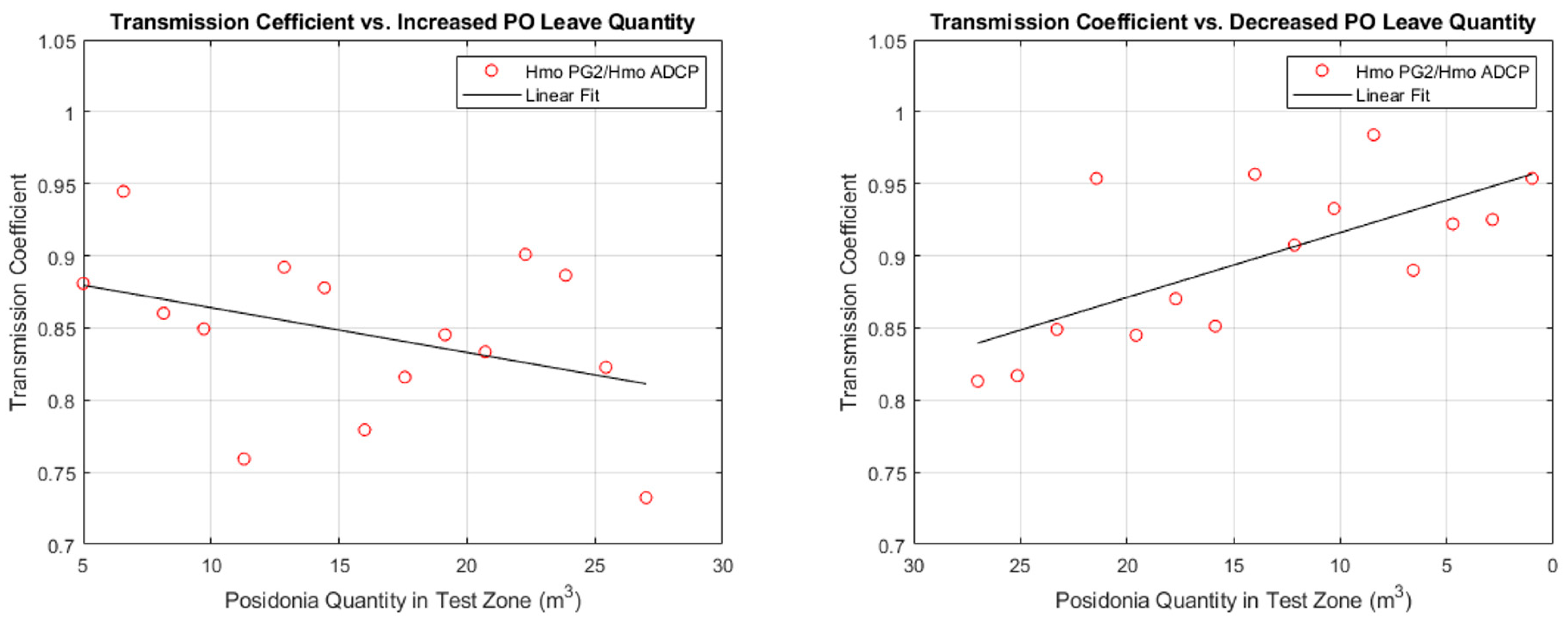
The transmission coefficient changed as the amount of PO leaves within the test zone changed (Figure 13). During the experiments, as the PO leaves continued to be released into the sea, the amount and concentration of PO leaves within the test zone increased. The graph on the left side of Figure 13 shows that the transmission coefficient decreased from 0.88 to 0.81 as the PO release reached its maximum. Later on, during the second half of the experiments, the PO release rate was matched and then surpassed by the rate at which PO leaves started escaping from the test area between the gauges, as shown on the right side of Figure 13. Here, the transmission coefficient again increased to approximately $K_t$ = 0.95, indicating a decreasing energy dissipation due to the reduced PO concentration in the test area. It should be noted that the amount of PO leaves could not be measured correctly within the testing zone, as they were continuously transported by the waves and currents. The amounts in Figure 13 were calculated from the volumetric estimates of the dumped material and the uniform release rates, as observed in the drone videos.

The frequency dependence of the dissipation phenomena was analyzed by calculating the transmission coefficients separately for three different frequency (period) bands, as shown in Figure 14 and Figure 15. For each frequency band, $H_{m_0}$ was calculated from the associated area of the zeroth spectral moment (m₀) within that particular frequency band and used for the $K_t$ calculation. Here, the $K_t$ values are plotted separately for the (a) long, (b) medium, and (c) short wave periods. Each figure shows the transmission coefficients for two cases. Figure 15 shows the wave transmission coefficients before a wave entered and after it left the PO zone (PG2/PG1). Long waves, with periods greater than 6.2 s, were less effected by the PO leaves (Figure 14a). Waves with periods between 4.5 and 6.2 s were strongly affected by the PO leaves, with $K_t$ values of less than 0.7. In this mid-frequency band, at which the peak energy was transmitted, the waves were not affected with the increased PO concentration, and dissipation was observed from the early stages of the test (Figure 14b). Short waves, with periods of 3.4–4.5 s, showed the strongest dissipation due to the PO field. The $K_t$ values for the PG2/PG1 dropped to 0.5, indicating the highest dissipation throughout the entire testing scheme. As the PO concentration increased, the leaves started to disperse offshore of the test area, thus causing both gauges, PG1 and PG2, to start showing dissipation with respect to the ADCP. Therefore, similarly high $K_t$ values were observed in both the PG1/ADCP and PG2/PG1 ratios (Figure 14c). The dissipation of waves was largest in the medium periods within the PO field and not very affected by the increase in the PO concentration as the release of leaves continued throughout the test. However, the short- and long-period waves were less affected by the PO leaves at the initial stage of testing. As the concentration of PO leaves increased, the short and long waves started to dissipate, of which the short waves were affected more than the long waves (Figure 15).

5. Conclusions and Further Study

In an experimental study conducted in the Eastern Mediterranean, the effects of natural PO leaves on reducing the incident wave heights that impact the beach were measured. The waves were electronically measured in nature on both the offshore and onshore sides of freely floating dead PO leaves using an underwater acoustic doppler current profiler and pressure gauges. The ADCP was located offshore at a 4 m depth, and the two pressure gauges were located on the offshore and onshore sides of the PO leaves at water depths between 0.5 and 0.8 m. The transmission coefficient, $K_t$, is defined as the ratio of the transmitted wave height divided by the incident wave height. The spectral wave parameters were obtained using a Fourier analysis of the time records, including the significant wave height ($H_{m_0}$) and the mean wave period ($T_{m_{0,2}}$).

The transmission coefficient ($K_t)$ was found to vary between 0.73 and 0.94, which is equivalent to a wave height decay of 6–27%. The results show that the free-floating dead PO leaves in their natural environment dissipated the incoming wave energy and had the capacity to protect the beach against erosion. Further analysis in separate frequency bands showed that medium period waves (with periods between 4.5 and 6.2 s) were more sensitive to PO leaves in terms of energy dissipation, whereas long waves (with periods of more than 6.2 s) were less sensitive. The transmission coefficient for the medium period waves was calculated using the medium-frequency part of the wave spectrum, delivering a maximum transmission coefficient of 0.5, corresponding to a 50% wave height decay due to PO leaves. It was concluded that the PO leaves operate like a band-pass filter on incoming waves and dissipate incident shorter waves more efficiently. On the other hand, the overall dissipation was much higher for medium periods (i.e., 4.5–6.2 s) for which the wave amplitudes were the highest. It can be concluded that high-amplitude waves were dissipated more than the others. The dissipation mechanism is partially in agreement with the formulation derived by Dalrymple et al. (1983) [5], who found a cubical relation between the dissipation rate and the wave amplitude. Therefore, in closed seas with shorter fetch and wave periods, PO leaves may work quite efficiently, similar to floating breakwater, which has similar transmission coefficients. Floating breakwaters are known to decrease shorter waves but let long waves pass. In the experiments, the maximum transmission coefficient for the PO leaves was found to be as low as 0.5. This value is equivalent to 75% wave energy dissipation, as the wave energy is proportional to the square of the wave height. Similarly, wave-induced beach erosion may drop by approximately 82% because of the higher exponent in the breaker height to sediment transport relation. In addition to the protection of beaches by reducing incoming wave energy, the accumulated PO leaves at the shore further protect the beach face by means of sediment trapping.

The defoliation of PO meadows in the Mediterranean Sea commences in autumn, followed by winter storms, which push the leaves ashore. This migration of free-floating dead PO leaves continues throughout the autumn and winter months, giving the PO leaves a prolonged duration of several months to spend in the nearshore zone. In the case of beaches open to waves, leaves washed ashore may return to the sea and continue to contribute to wave dissipation in cycles. Therefore, to understand the overall dissipation capacity, in future studies, it is suggested to investigate the transport and fate mechanisms of fallen PO leaves.

The present study has several limitations, including the exact amount and distribution of the PO leaves between the gauges. However, the obtained results can still be used to verify existing and/or new models that simulate the energy dissipation of the bulk-dissipative behavior of dead free-floating PO leaves.

For future scientific work, it would be practical to perform wave basin tests with fallen PO leaves. The use of real leaves instead of imitations can provide realistic results that can represent PO in nature and can help develop better models and parameters.

Based on the promising outcomes of this research regarding the wave dissipation capacity of PO leaves in their natural environment, it is recommended that local authorities should stop disposing of PO leaves washed ashore on beaches and promote the use of PO as a nature-based solution to combat beach erosion around the world.