Article

Optimal Coordinated Operation for Hydro–Wind Power System

1
School of Water and Environment, Chang’an University, Xi’an 710054, China
2
Yalong River Hydropower Development Company, Ltd., Chengdu 610065, China
*
Author to whom correspondence should be addressed.
Water 2024, 16(16), 2256; https://doi.org/10.3390/w16162256
Submission received: 3 July 2024 / Revised: 2 August 2024 / Accepted: 7 August 2024 / Published: 10 August 2024

Abstract

The intermittent and stochastic characteristics of wind power pose a higher demand on the complementarity of hydropower. Studying the optimal coordinated operation of hydro–wind power systems has become an extremely effective way to create safe and efficient systems. This paper aims to study the optimal coordinated operation of a hybrid power system based on a newly established Simulink model. The analysis of the optimal coordinated operation undergoes two simulation steps, including the optimization of the complementary mode and the optimization of capacity allocation. The method of multiple complementary indicators is adopted to enable the optimization analysis. The results from the complementary analysis show that the hydraulic tracing effect obviously mitigates operational risks and reduces power losses under adverse wind speeds. The results from the analysis of capacity allocation also show that the marginal permeation of installed wind capacity will not exceed 250 MW for a 100 MW hydropower plant under random wind speeds. These simulation results are obtained based on the consideration of some real application scenarios, which help power plants to make the optimal operation plan with a high efficiency of wind energy and high hydro flexibility.

1. Introduction

The undesired environmental impact of combustion-based electricity provides an important opportunity for reforming the energy structure [1,2]. Renewable energy sources (RESs) are progressively occupying a larger share of the energy mix [3,4]. Among the abundant RESs, the power potential of wind energy exceeds all other electricity consumptions in the world [5]. For instance, wind energy contributes up to 50% of the installed renewable capacity in Australia [6] and accounts for 40% of the domestic electricity generation in Germany [7]. On the other hand, hydropower is one of the most stable RESs, making it an ideal counterpart to regulate the power fluctuations in integrated power systems [8]. Hydropower and wind power generation have great development potential, which will maintain an upward tendency to 2030 (as shown in Figure 1) due to their huge benefits for the environmentally friendly and sustainable electricity industry [9]. Due to the intermittent and stochastic characteristics of wind power, the optimal coordinated operation of hydro–wind-based power systems becomes more important for the efficient use of energy.
In examining the literature, there are three ways to achieve the optimal coordinated operation of hydro–wind-based power systems. The first is establishing an optimization model to optimize the operating coefficients, with the optimized results revealed by the model outputs or transformed forms of these model outputs. In other words, the established model is able to simulate the dynamic operation characteristics of a power system over time. The key to this is to establish an appropriate optimization model, as such a model can reflect the coupling characteristics of each component or subsystem. For instance, Zhang et al., (2019) [10] proposed a hydro–wind–photovoltaics optimization model to calculate the optimal coefficients of coordinated operations in different seasons. Ju et al., (2022) [11] proposed a fully distributed power flow calculation method for the coordinated operation of hybrid microgrids. Simiao and Ramos (2020) [12] presented a hydro–wind–photovoltaics optimization model to optimize the cost and reliability indices. Mou et al., (2023) [13] constructed a fault diagnosis model for intelligent dispatching energy storage systems based on a deep learning algorithm. Alvarez and Ronnberg (2018) [14] established a reservoir-type hydropower equivalent model for hydro–wind–thermal power systems to optimize the coordinated operation of multiple energies. The second way to achieve the optimal coordinated operation is by designing an operational optimization method or scheduling method to maximize the benefits of operation goals. This mostly uses linear/nonlinear programming methods to establish objective functions and constraints without the need to build complex mathematical models of the various components of power systems. The coverage of objective functions and the comprehensiveness of constraints are the key points of this approach to the evaluation of optimizing operations. For instance, Meng et al., (2024) [15] proposed an optimal scheduling strategy for hybrid power systems that can combine distributionally robust optimization and Stackelberg game theory. Zhu et al., (2024) [16,17,18,19] applied a series of novel optimization methods, like the three multi-objective optimization method and the multi-objective grey wolf optimization technique, to achieve the optimal operating mode of hybrid power systems. Li et al., (2022) [20] developed a continuous-time distributed algorithm for the economic dispatch problem of a power–water network. Guo et al., (2022) [21] proposed the risk-averse day-ahead optimization scheduling of hydro–wind–photovoltaic power systems, considering the steady requirement of power delivery. Majumdar et al., (2021) [22] achieved hydro–wind–photovoltaics–thermal scheduling based on the method of Mayfly algorithm optimization. Wang et al., (2017) [23] presented an improved hybrid method based on biogeography/complex and metropolis for many-objective optimization. Zhang et al., (2021) [24] presented the long-term optimization scheduling of a hydro–wind power system. The third way is optimizing the complementary performance of fluctuations in output power or frequency. This method emphasizes in-depth excavation from a certain research perspective, which generally includes controller optimization and the optimization of operation variables or scenarios. Regarding controller optimization, Shirkhani et al., (2023) [25] summarized microgrid decentralized energy/voltage control methods. Saidi et al., (2016, and 2011) presented passivity-based direct power control of the shunt active filter [26], a method for the quality improvement of the shunt active power filter [27], and shunt active filter control based on adaptive fuzzy logic [28]. Regarding the optimization of operation variables or scenarios, Avila et al., (2021) [29] evaluated hydro–wind complementarity in medium-term planning from the viewpoint of the periodic stream flow and wind speed time series. Liu et al., (2024) [30] studied the performance, pricing, and coordination of a hybrid system from a data security perspective. Fayek and Kotsampopoulos (2021) [31] optimized the complementary performance of hybrid power systems from the viewpoint of frequency deviation. Ren et al., (2022) [32] investigated hydro–wind–photovoltaics complementarity from the viewpoint of fluctuations in power output. Tang et al., (2020) [33] optimized the sizes of renewable power plants for a hydro–wind–photovoltaics power system based on the power output complementarity. Table 1 is used to clearly show the differences in the above three ways of achieving the optimal coordinated operation.
Compared with the former two ways, the third way has the advantage of a small amount of calculation. In addition to this, the third way flexibly reflects the coordinated operation of hydro–wind-based power systems, since there are various complementary indicators. It is summed up through the above literature review that these complementary indicators mainly include frequency deviations, the volatility of power outputs, and other indicators with fluctuations. These complementary indicators have been applied separately in the existing literature, but several studies have comprehensively considered coordinated operations with multiple indicators. Moreover, the power loss in this paper is adopted as a newly added indicator to participate in the multi-indicator optimizing operation of a hydro–wind power system.
Based on the above considerations, this paper studies the optimal coordinated operation of a hydro–wind power system by considering multiple complementary indicators. The detailed complementary indicators involve the hydraulic tracing power, the volatility of wind power, the fluctuations in hydraulic frequency, and the power loss. By fully considering the need for actual power plants, the optimal coordinated operation of the hybrid system includes two aspects: (i) the optimal complementary mode between hydro and wind power, and (ii) the optimal capacity allocation of wind power. The optimal complementary mode is analyzed under two real application scenarios, including the on-demand hydropower scenario and the surplus hydropower scenario. Among them, the on-demand hydropower scenario means that the planned electricity produced by the stations is equivalent to the demand of the daily load. The surplus hydropower scenario is an operating condition where the planned electricity is larger than the demand of the daily load. The analysis is conducted by using the software of Matlab 2023b. The simulation results from the complementarity analysis will help the hybrid power plant to stimulate the best regulation capability. Similarly, the simulation results from the analysis of the optimal capacity allocation will contribute to the maximum utilization of wind energy.
The novelties of this paper are summarized in two aspects. (i) A relatively complete model of the hydro–wind hybrid power system is established based on their rigorous mathematical relationship. In this hybrid model, the hydropower subsystem considers the dynamic characteristics of all major hydraulic–mechanical–electrical components, and the wind power subsystem adopts Type IV wind turbines (WTs) to better adapt to changes in wind speed. This hybrid model facilitates the research of numerical simulations. (ii) Multiple complementary indicators, particularly power loss, are comprehensively considered to achieve the optimal coordinated operation of the hybrid power system, helping to improve the reliability of the evaluation results. Correspondingly, the benefits of this study are concluded as: (i) The proposed assessment method that constructs multi-type optimization indicators based on the real-time outputs of the simulation model fills a major gap in previous investigations. (ii) The applicability of the proposed method can be extended to most hybrid power systems involving hydropower, which contributes to enhancing energy efficiency by maximizing the dynamic regulation benefits of hydropower. (iii) The results obtained in this work can be effectively used by energy engineers to improve the operational stability and economic benefits of power stations.
This paper is structured as follows: Section 2 models the hydro–wind power system. Section 3 presents the methodology. Section 4 optimizes the complementary mode. Section 5 optimizes the capacity allocation to maximize the power generation. The conclusions and discussion in Section 6 summarize the paper.

2. Model

The working mechanism of the integration of hydropower and wind power systems is shown in Figure 2, and its detailed modeling is discussed in the following subsections.

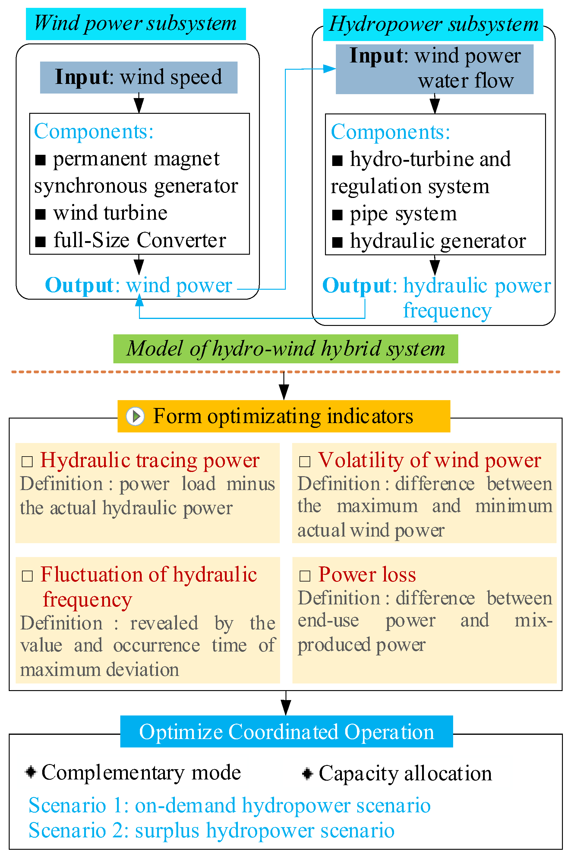
2.1. Wind Power System

The wind power model adopts a Type IV wind turbine, which has a directly coupled permanent magnet synchronous generator (PMSG). The PMSG is composed of various converters.

2.1.1. Wind Turbine

The wind turbine (WT) converts the kinetic energy into mechanical power, and it is expressed as [34]:
P t = 1 2 ρ A v 3 C p ( λ , β ) ,
where ρ, A, and v denote the air density, swept area of blades, and wind speed (m/s), respectively. Cp is the wind power coefficient, represented by the blade pitch angle β and tip–speed ratio λ. The tip–speed ratio λ is the ratio of the blade tip linear speed to the wind speed. The longer the blade or the faster the blade speed, the higher the tip–speed ratio in the same wind speed conditions. The tip–speed ratio λ [35] is written as:
λ = t/v,
where R and ωt are the radius of the blade (m) and rotational speed of the wind turbine (rad/s).
The relationship between the tip–speed ratio λ and the blade pitch angle β is related to the maximum wind power coefficient Cpmax, as described in Figure 3 [35].
The extraction of the maximum power from the wind turbine depends on the maximum value of the wind power coefficient Cp(λ, β), and this maximum value is defined as:
C p max ( λ , β ) = i = 1 n i = 1 n α i j λ i β j .

2.1.2. PMSG

The PMSG directly connects to the wind turbine, and this configuration can reduce noise, mechanical loss, and fault probability and also improve efficiency. The stator voltage in the synchronously rotating d-q frame [36,37] is expressed as:
u s d = R s i s d + d ψ s d d t ω e ψ s q u s q = R s i s q + d ψ s q d t ω e ψ s d ,
where us, is, Rs, ψ s , and ωe are the voltage, current, stator resistance, magnetic flux, and rotor speed of the generator, respectively. Subscripts d and q refer to the d-axis and q-axis, respectively.
The magnetic flux of the stator in the d-axis and q-axis is written as:
ψ s d = L d i s d + ψ 0 ψ s q = L q i s q ,
where ψ 0 is the magnetic flux of the permanent magnet. Ld and Lq are the d-axis and q-axis inductances, respectively. The electromagnetic torque of the PMSG is expressed as:
Te = 1.5n(ψ d iqψ q id),
where n is the pole pair. If Ld = Lq = L, Equation (6) can be transformed into the following form:
Te = 1.5nψ 0isq.

2.1.3. Full-Size Converter

The full-size converter is composed of the diode rectifier, DC–DC boost converter, and VSC. The diode rectifier is used to track the maximum power of the wind turbines. The DC–DC boost converter avoids the failure of voltage rectification under undesired wind speeds. The boost converter adjusts the input current on the rectifier side, which reduces harmonic pollution. The mechanism of the DC–DC boost converter [38,39] is described as:
d u d c d t = 1 C u d c ( u g i g + u s i s P l ) u g i g = u g d i g d + u g q i g q u s i s = u s d i s d + u s q i s q ,
where ugd and igd are the d-axis voltage and current on the grid side. ugq and igq are the q-axis voltage and current on the grid side. udc is the DC link voltage. Pl is the total active power loss.
The VSC is essentially a grid-side inverter which maintains the stability of the DC link voltage. The VSC’s equation is generally expressed as:
u g d = R g i g d L g d i g d d t + ω g L g i g q + e g d u g q = R g i g q L g d i g q d t ω g L d i g d ,
where Rg and Lg are the line resistance and inductance, respectively. ωg and egd denote the synchronous angular speed of the grid and the grid voltage in the d-axis, respectively.
According to refs. [40,41], the block diagram of the full-size converter is modeled in Figure A1 (see Appendix A).

2.2. Hydropower System

The hydropower system includes a Francis hydro-turbine, synchronous generator, frequency-governing system, and pipe system. The utilization mode of water energy of Francis hydro-turbines belongs to the reaction type. The operating head of Francis hydro-turbines is in the range from 20 to 700 m, and the corresponding hydropower system is suitable to be built in the river section with slow gradients and a large discharge. Hydropower regulates intermittent wind power and maintains the reliability of the power system. Its detailed modeling is shown in the following subsections.

2.2.1. Pipe Characteristic

Considering the elastic characteristic of the pipe wall, the dynamic characteristic of the pipe [42] is described as:
G D ( s ) = h ¯ q ( s ) q ¯ ( s ) = b 3 s 3 + b 2 s 2 + b 1 s + b 0 a 2 s 2 + a 1 s + a 0 ,
where GD(s) is the transfer function between the turbine head and flow, h ¯ q (s) is the head variation, and q ¯ (s) is the flow variation. The coefficients in Equation (10) are further expressed as:
a 0 = 24 h w ,   a 1 = 6 T r h f ,   a 2 = 3 T r 2 h w b 0 = 24 T r h w h f ,   b 1 = 24 T r h w 2 ,   b 2 = 3 T r 2 h w h f ,   b 3 = T r 3 h w 2 ,
where hw is the pipe characteristic coefficient, Tr is the water hammer time constant, and hf is the hydraulic friction loss.
Based on the Laplace transform of GD(s) [43,44], the turbine head and flow are finally obtained as:
h q = 1 f p q 2 q 2 y 2 q = q 0 + q ¯ = a 2 x 3 + a 1 x 2 + a 0 x 1 + q 0 ,
where q0 and y are the relative values of the initial flow and guide vane opening. The state equation of Equation (12) is described as:
x ˙ 1 = x 2 x ˙ 2 = x 3 x ˙ 3 = b 0 b 3 x 1 b 1 b 3 x 2 b 2 b 3 x 3 + 1 b 3 h q .

2.2.2. Hydraulic Generator

The electromotive force equation of the synchronous generator [45] is expressed as:
E ˙ 0 = U ˙ + r a I ˙ + j I ˙ d x d + j I ˙ q x q x d = x a d + x σ x q = x a q + x σ ,
where E0 is the excitation electromotive force. U is the terminal voltage. xd and xq are the d-axis and q-axis synchronous reactance. xad and xaq are the d-axis and q-axis armature reactance. ra is the armature resistance. xσ is the magnetic flux leakage.
The electromagnetic power of the synchronous generator is expressed as:
P e m = m E σ I cos φ i ,
where m is the phase number of the stator. φ is the power factor angle. φi is the phase angle between the air gap voltage and the armature current. The output power of the generator is derived from the difference between the electromagnetic power (Pem) and armature copper loss (PCu), which is:
P o u t = P e m P C u P C u = m I 2 r a .
The power and torque relationship is expressed as:
P i n Ω = P 0 Ω + P e m Ω ,
where Ω is the mechanical rotor speed, Ω = 2πn/60. Pin and P0 are the input power of the generator and no-load loss, respectively. Equation (17) is further represented by the electromagnetic torque, i.e.,
M i n = M 0 + M ,
where Min is the input mechanical torque of the generator, M0 is the no-load torque, and M is the electromagnetic torque.
Ignoring the armature copper loss PCu, the power angle characteristic of the generator is:
P e m = m E 0 U x d sin θ + m U 2 2 ( 1 x q 1 x d ) sin 2 θ ,
where θ is the power angle.
Similarly, the reactive power of the generator is:
Q e m = m E 0 U x d cos θ m U 2 2 x d + x q x d x q + m U 2 2 x d x q x d x q cos 2 θ .

2.2.3. Hydro-Turbine and Frequency Regulation System

Generally, hydro-turbines are defined by mechanical torque and flow. These variables are further represented by the guide vane opening, rotational speed, and turbine head. The dynamic characteristic of hydro-turbines [46] is, therefore, described as:
M t = M t ( y , h , n ) Q t = Q t ( y , h , n ) ,
where Mt, Qt, h, y, and n are the mechanical torque, flow, head, guide vane opening, and rotational speed, respectively. Equation (21) can be further expressed by the relative values of Mt and Qt, i.e., the relative flow q and relative mechanical torque mt. It is expressed as:
m t = e x x + e y y + e h h q = e q x x + e q y y + e q h h ,
where ex, ey, and eh are the relative deviations of the mechanical torque with respect to the rotational speed, the guide vane opening, and the turbine head, respectively. eqx, eqy, and eqh are the relative deviations of the flow with respect to the rotational speed, the guide vane opening, and the turbine head, respectively.
The dynamic performance of hydro-turbines is governed by the PID controller, which is also used to achieve the desired frequency regulation. The conventional PID controller [47] is adopted as:
Y p i d ( s ) Δ F ( s ) = ( K p + K i s + K d s T n + 1 ) ,
where Ypid(s) is the Laplace transform of the guide vane opening. ΔF(s) is the Laplace transform of the frequency. Tn is the acceleration time constant. Kp, Ki, and Kd are the proportional, integral, and differential adjustment coefficients, respectively.
Based on Equation (23), the electro-hydraulic servo system is expressed as:
Y ( s ) Y p i d ( s ) = 1 T y s + 1
Based on the above descriptions, a block diagram of the hydro-turbine and frequency regulation system is shown in Figure A2 (see Appendix A). A description of the setting of the PID control parameters is shown in Appendix B.

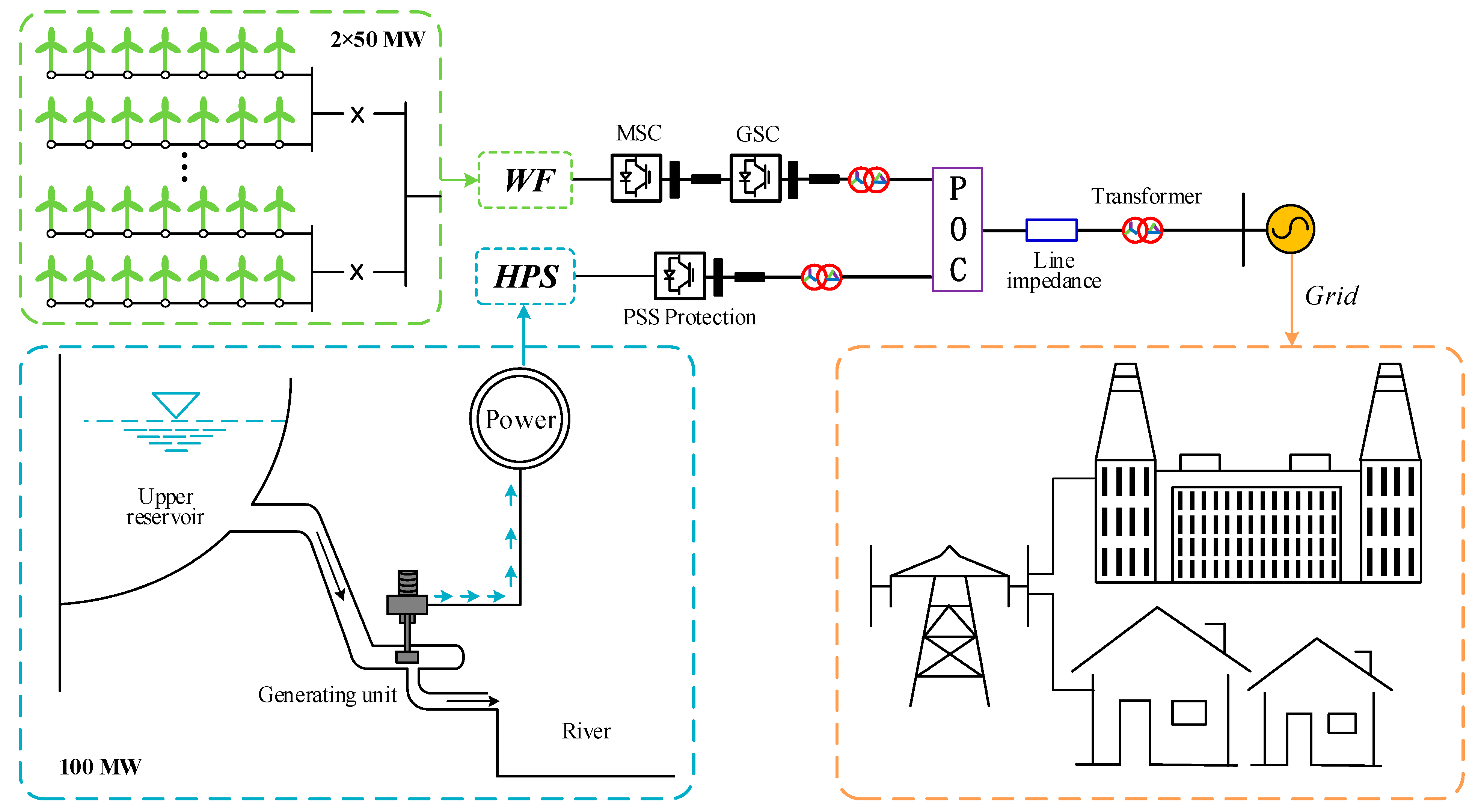
2.3. Hybrid Power System

A hybrid model of the hydro–wind power system is shown in Figure A3 (see Appendix A). In this integrated model, the capacity of the single-machine wind turbine is 2 MW and the rated frequency is 60 Hz. The total installed capacity of the wind farm is 100 MW, with 50 wind turbines. The generation capacity of the hydropower system is 100 MW, and its load reserve capacity is 3 MW. The hydropower and wind power connect to the power grid through two transformers. The load demand of the power grid is 200 MW, which equals the total installed capacity of the hybrid system.

3. Methodology

Based on the established mathematical model of the hydro–wind hybrid power system in Section 2, the hydraulic power, wind power, and hydraulic frequency are output by the model. According to these outputs, four complementary indicators, including the hydraulic tracing power, volatility of wind power, fluctuations in hydraulic frequency, and power loss, are obtained to optimize the coordinated operation of the hybrid system. The definitions of these four indicators are described in Table 2. The optimization methodology is shown in Figure 4.

4. Optimization of Complementary Mode

This section aims to maximize the total power generation by optimizing the complementary mode. The analysis is conducted based on two operating scenarios, including the on-demand hydropower scenario (Scenario 1) and the surplus hydropower scenario (Scenario 2). Table 3 describes the characteristics of these two scenarios. Three basic types of wind speeds are considered to optimize the complementary characteristics of the hybrid system, including constant, mutational, and random winds [48,49,50,51]. A constant wind speed reflects changes in the average wind speed in the wind field, which mainly determines the rated power delivered by the wind generator to the hydro–wind power system. A mutational wind speed can simulate sudden changes in wind speed, which is generally used to assess the degree of power and voltage fluctuations under large changes in wind speed when analyzing the influence of the wind power system on the stability of the power grid. A random wind speed can simulate the characteristics of random fluctuations in wind speed, which influence the stability of the wind power output. For the sake of analysis, constant wind speed, mutational wind speed, and random wind speeds are abbreviated as wind type 1, wind type 2, and wind type 3. The waveforms of these three wind speeds are shown in Figure 5a. The transmission power loss is finally calculated to reflect the differences in power generation under the three wind speeds.

4.1. Scenario 1: On-Demand Hydropower Operation

In Scenario 1, hydropower is considered as a regulator to regulate fluctuations in wind power. Also, it is used to complement electricity shortages of the power grid. The complementary characteristic is investigated under three types of wind speeds, as shown in Figure 5a. The corresponding power structure is shown in Figure 5b.
In Figure 5a, it is observed that the hydraulic power and wind power show opposite trends under the three wind conditions. This means that hydropower has an excellent complementary effect on regulating fluctuations in wind power, since the sum of the hydraulic power and wind power is close to the power requirement. There are some major differences in the complementary characteristics, which are mainly manifested in the power variation in the magnitude and trends under the three wind speeds. The relative wind power for the constant wind fluctuates slightly between 1 and 0.986. Conversely, the relative wind power for the mutational wind displays a large fluctuation from 1 to 0.3751. From the perspective of power fluctuations, the mutational wind has a relatively larger influence on the operating safety of the power system. However, hydraulic power closely tracks fluctuations in wind power, which can help to mitigate operating risks under mutational wind conditions.
In Figure 5b, the power gap is the negative difference between the power demand of the grid and the power generation of the hybrid system, while the surplus power is the positive difference. The coordinated operation of the hybrid system shows a promising power structure in the random wind speed condition (Type 3). The main reason behind this is the relatively less surplus power under Type 3 in comparison to the large power under the constant wind (Type 1). The surplus power produced in Type 1 is due to the inappropriate and sub-optimal complementary mode of hydro and wind energies. Moreover, compared with the mutational wind (Type 2), the power gap is relatively less under Type 3. The power gap produced in Type 2 is attributed to it being the most unfavorable wind condition.
For a hybrid power system, transmission power loss is generally unavoidable, and it will reduce the amount of electricity available to users. For this reason, the end-use power consumption of the power grid is likely to be less than the mix-produced power of the hybrid system. Figure 6a shows the influence of the three wind speeds on the end-use power and mix-produced power, and Figure 6b shows the corresponding power loss obtained from the difference between the mix-produced power and end-use power.
In Figure 6, the end-use power changes slightly by around 194.5 MW for Type 1 and 3 winds, and the corresponding total power generation changes by around 201 MW. The end-use power and total power generation for Type 2 change significantly compared to the power for Type 1 and 3 winds. This means that Type 2 produces the worst wind conditions for the coordination operation of the hybrid power system, since the power loss is the largest among the three wind speeds. Moreover, it is worth noting that the end-use power under different wind speeds is always less than the power demand of the grid (i.e., 200 MW). This is caused by the unexpected power loss in the transmission process. As shown in Figure 6, the power loss continuously changes throughout the whole operating cycle (i.e., 0 s to 30 s). Compared to Type 1 and 3 winds, the power loss for Type 2 wind is relatively large and reaches a maximum of 6.83 MW. On the other hand, the mean power loss for Type 1 and 3 winds is roughly around 6 MW.

4.2. Scenario 2: Surplus Hydropower Operation

In Scenario 2, the power demand of the grid changes from 200 MW to 150 MW. The hydro generator in this scenario mainly acts as a regulator to suppress wind power fluctuations. The results of the complementary characteristics of the hydro–wind power system are shown in Figure 7a.
The hydraulic tracing power is defined as the difference between the power consumption and the actual hydraulic power. There is an excellent complementary mode if the hydraulic tracing power is approximately consistent with the variation in the actual wind power under the wind speed. As shown in Figure 7a, the complementary mode between the hydro and wind power systems is excellent in Scenario 2. The hydraulic tracing power sees small variations under Type 1 wind, while the mutational wind triggers large power fluctuations. In particular, the wind power decreases to a minimum of 6.56 MW, which obviously reduces the efficiency of the power system. However, this insufficient power capacity can be supplemented by hydropower without consuming additional reserve capacity. Type 3 wind causes the wind power to decrease from 100 MW to 77.54 MW. Such a big variation cannot influence the overall power generation capability of the power system due to the timely tracing of the hydropower. However, power loss may exist in Figure 7a, because the curve of the hydraulic tracing is almost coincidental with the curve of the wind power. For this reason, Figure 7b shows the variation trend of power loss.
Figure 7b shows the hydraulic tracing effect and power loss in Scenario 2. It reveals that the maximum power loss (4.68 MW) for Type 2 wind is larger than that for Type 1 wind (4.64 MW) and Type 3 wind (4.63 MW). The corresponding mean power loss for the Type 2 wind is the lowest (3.98 MW) due to the small amplitude of the fluctuations in the power loss. However, the mean power loss for the other two wind types is relatively small.
Compared with Scenarios 1 and 2, the wind volatility is almost similar in different wind conditions, and the hydraulic tracing effects are generally excellent for all wind types. To better compare the complementary characteristics in the two operating scenarios, the obvious differences in power loss enable this analysis. It is clearly shown that there are massive power losses produced in Scenario 1 compared to the operation in Scenario 2. The main reason behind this is the high demand for the power of the grid in Scenario 1 relative to Scenario 2. Specifically, the mean and maximum power loss for Scenario 1 are 6 MW and 6.8 MW, while for Scenario 2, they are around 4 MW and 4.6 MW, respectively. The occurrence time of the maximal power loss for these two scenarios is between 1 s and 3 s, which is caused by the power regulation capability of the hydropower at the initial coordinated operating stage.

5. Optimization of Capacity Allocation

This section is dedicated to increasing the total power generation by optimizing the capacity allocation of hydro and wind energies. From Section 4, it is obtained that Type 2 wind is the most unfavorable wind condition, since it leads to greater power loss than the other types of wind speed. Considering this, the capacity allocation under the wind type 2 wind is emphasized in this analysis. The number of WTs is 50, corresponding to the installed wind capacity of 100 MW, as studied in Section 4. The results obtained from Section 4 clearly show that 50 WTs is not the marginal permeation of the installed wind capacity when the hybrid power system begins to lose its stability. For this reason, the initial studied number of WTs starts from 51 in this section. The selected number of WTs is finally 51, 55, 60, and 61 corresponding to the installed wind capacities of 102 MW, 110 MW, 120 MW, and 122 MW. In this optimized analysis, the effect of the WTs’ number on the hydraulic suppression effect is first studied, and the power loss is then compared under the three wind types.
The most unexpected wind is Type 2 wind, as discussed earlier in Section 4. For this reason, Type 2 wind is considered in this analysis to optimize the capacity allocation. The result of the hydraulic suppression effect is shown in Figure 8, and the result of the power loss is shown in Figure 9.
Figure 8a shows the power complementarity and fluctuations in hydraulic frequency. It is observed that the wind power fluctuation gradually increases with an increase in WT numbers. Despite this, the hydraulic frequency cannot exceed ± 0.5 Hz, which is an accepted range for the power grid. Figure 8b shows the out-of-control hydraulic frequency that denotes ineffective regulation of the hydropower system at this instant. The out-of-control point (OCP) of the hydraulic frequency is the time where the hydropower system starts to lose its stability. For the power system with 61 WTs, the OCP occurs at 21.65 s, and its hydraulic frequency infinitely closes to 0.5 Hz. The wind power is out of control when its relative value decreases to 0.35 at 21.65 s.
Figure 9 shows the effect of capacity allocation on the power loss under Type 2 wind. As depicted in Figure 9, there always exists surplus power at 1.95 s with an increase in WT numbers, and the corresponding value of the surplus power shows an increasing trend from 2.2 MW to 2.8 MW. The power gap also increases when the WT number changes from 51 to 60. This is caused by the increasing fluctuation of wind power with the permeation of the installed wind capacity. The power loss continuously changes, influenced by the mutational wind in the whole production process. This reveals that the quantity of the power loss is closely related to the capacity allocation of hydro and wind energies.
Table 4 clearly reveals the detailed quantities of power losses under the three wind speeds. For Type 1 wind, the hydraulic frequency exceeds ± 0.5 Hz until 164 WTs, and the state of OCP is maintained around five seconds. This means that the hydropower rapidly loses the regulation effect on balancing wind power fluctuations when the installed wind capacity approaches the adjustable marginal permeation. For Type 2 and 3 winds, from the OCP perspective, the marginal permeation values of the installed wind capacity are 61 WTs and 127 WTs. From this angle, it is found that Type 1 wind has a great capability to adapt wind energy to the power grid, and the capability of Type 2 is the worst.
Moreover, owing to the hydraulic suppression effect, the complementary characteristic of the hybrid system is excellent or good before the occurrence of the OCP. The mean and maximum power loss show an increasing trend with an increase in WT numbers, and the peak loss occurs in the first second. Comparing the three wind speeds, the growth rate of the power loss is the fastest for Type 2 wind, followed by Type 3 wind and Type 1 wind. Note that the power loss is small at 60 WTs for Type 2 wind. In this situation, the critical wind permeation is determined by the considerably high hydraulic frequency. When the accepted WT number for Type 1 wind reaches 163 and the number for Type 3 wind reaches 125, the corresponding mean power loss exceeds 20 MW. In this situation, the critical wind permeation is determined by the rate between the mean power loss and the installed wind capacity. Correspondingly, the rates for these two winds are 5.12% and 5.57%, respectively. Thus, comprehensively considering the power loss, complementary characteristics, and hydraulic regulation capability, the critical wind permeation values for Type 1, 2, and 3 are 326 MW, 120 MW, and 250 MW with respect to 163, 60, and 125 WTs.

6. Conclusions and Discussion

This work studies the optimal coordinated operation of hydro–wind power systems by establishing multiple complementary indicators. The power loss is different from previous investigations, as it is a newly presented indicator in the optimization method. Apart from the power loss, the other complementary indicators include the hydraulic tracing power, the volatility of wind power, and the fluctuations in hydraulic frequency. All these four indicators are constructed from the output variables of the established model. The analysis encompasses both the optimal complementary mode and the optimal capacity allocation, with the consideration of two real application scenarios, including the on-demand hydropower scenario and the surplus hydropower scenario. The key findings from this study include the following:
(1)
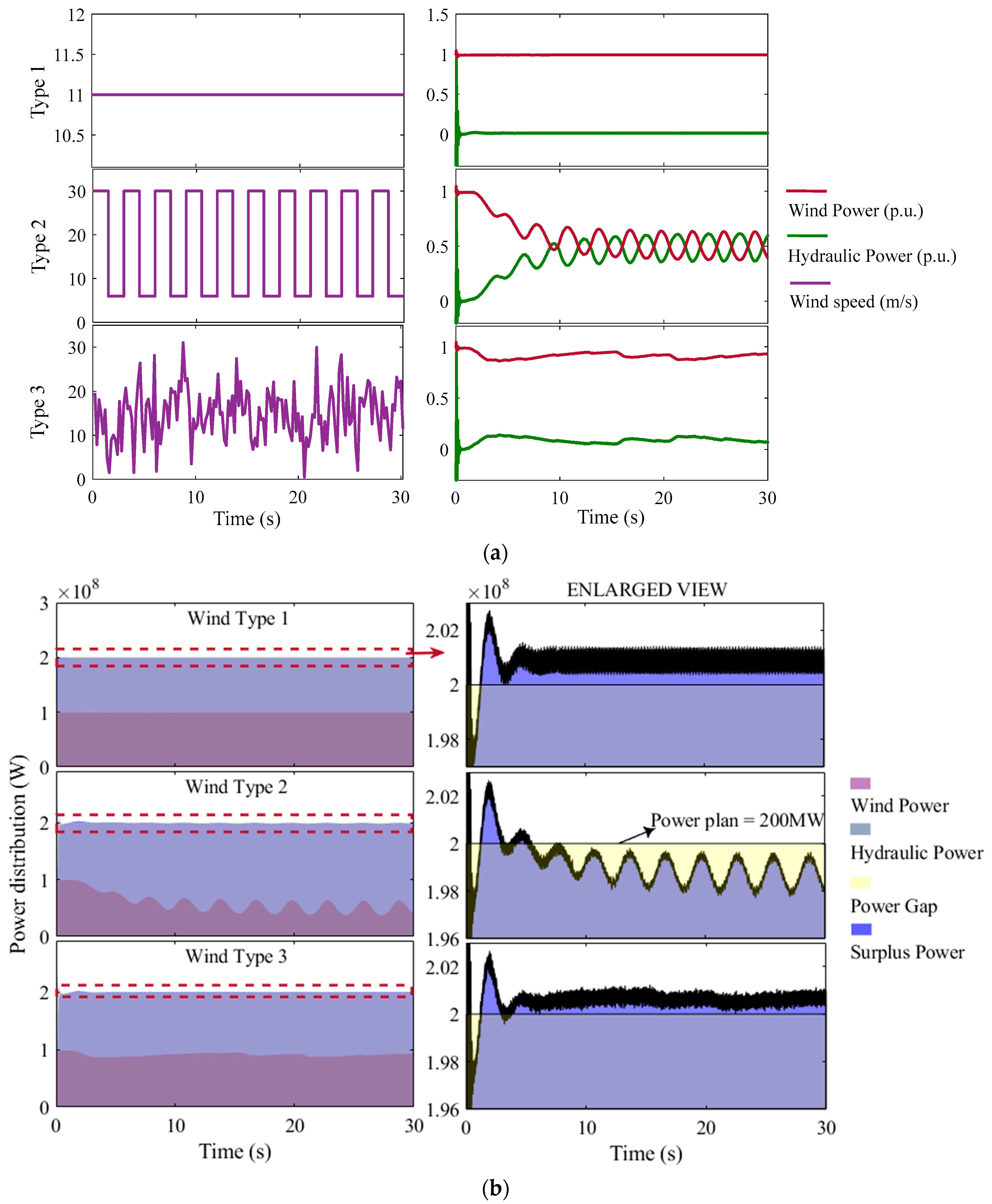
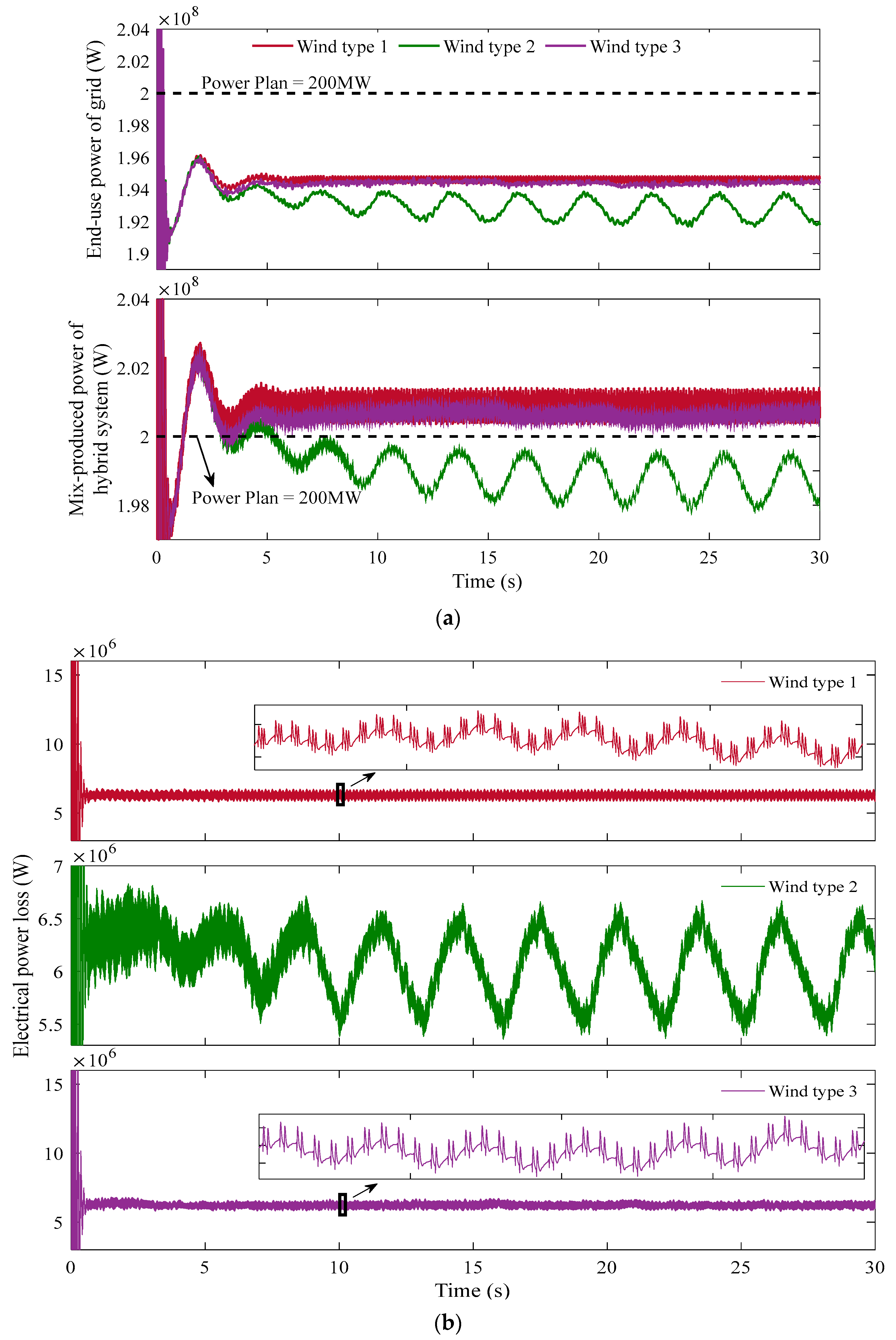
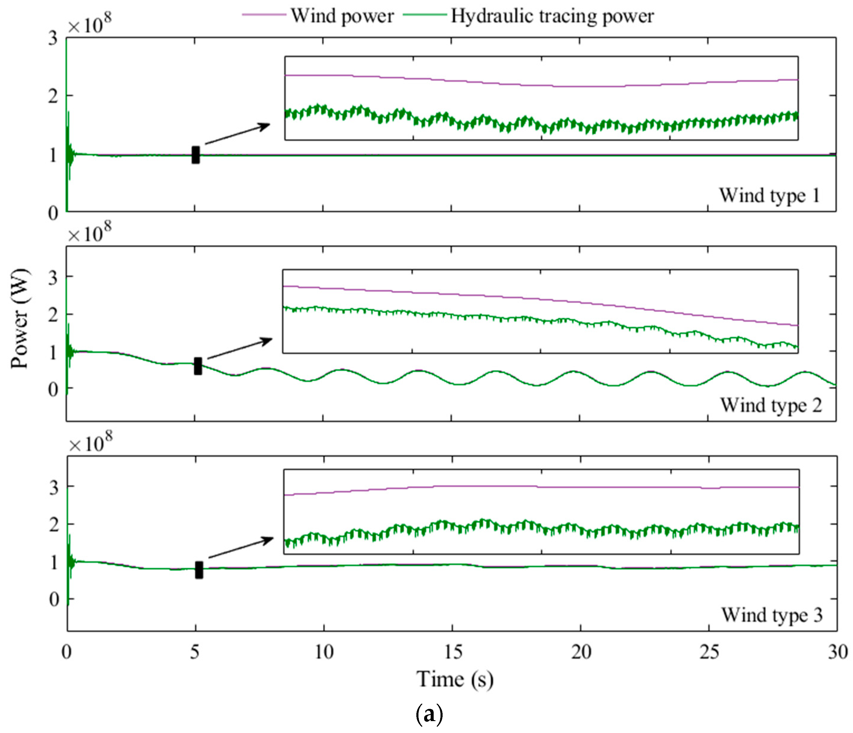
The effect of wind speeds on the complementary mode: The mutational wind speed causes the worst complementary mode of the power system because there is an increasing burden of hydro regulation to cope with frequently drastic changes in wind speed. On the contrary, the complementary mode is the best under the random wind speed, since the power system makes full use of the regulation capability of hydropower in this situation.
(2)
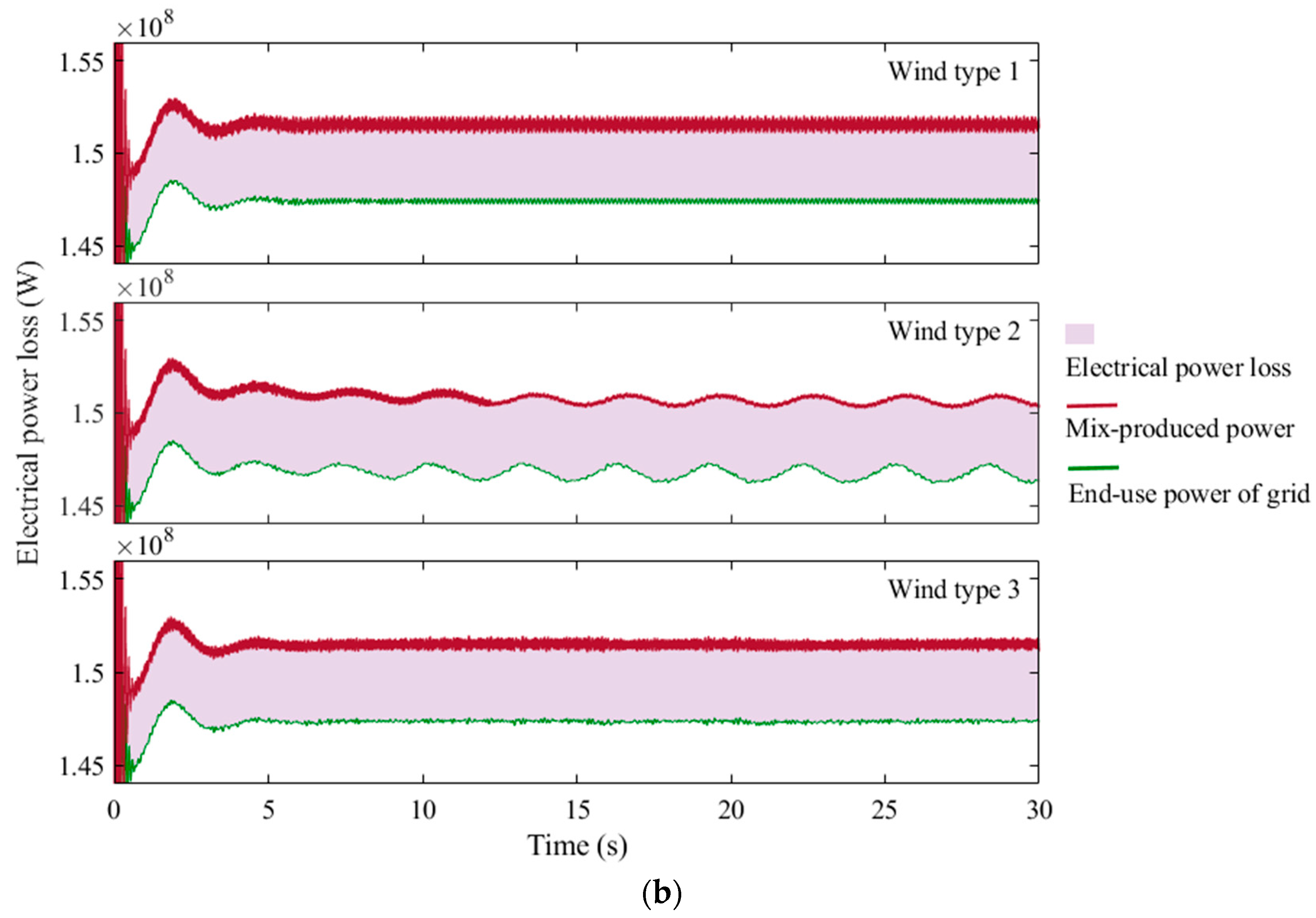
The effect of application scenarios on the complementary mode: The most distinctive feature of complementarity for both real application scenarios lies in the power loss. The mean power loss for the on-demand hydropower scenario is 6 MW, while that for the surplus hydropower scenario is around 4 MW. Thus, the on-demand hydropower scenario is a better choice for the economic operation of power stations from the perspective of power loss.
(3)
The necessity for multiple indicators: When the hybrid power system is close to instability with the increasing wind power permeation, the marginal permeation of the installed wind capacity cannot be determined by a single indicator. For instance, the system loses stability when the hydraulic power and wind power still have good complementary tracking effects. In this situation, the indicators of power loss and hydraulic frequency are able to reveal this instability.
(4)
The optimal capacity allocation: Based on the comprehensive evaluation of multiple indicators, the marginal permeations of the installed wind capacity for a 100 MW hydropower system are approximatively 326 MW, 120 MW, and 250 MW under constant, mutational, and random wind speeds.
The optimal coordinated operation in this paper is conducted based on complementary indicators. For a deeper investigation, future work will try to establish an optimization method represented by objective functions and constraints to study the optimal coordinated operation of hybrid power systems, and it will also be compared with some modern algorithms like the Mountain Gazelle Optimizer in ref. [52].

Author Contributions

Conceptualization, H.L. and T.L.; data curation, H.L. and Z.Z.; formal analysis, H.L. and H.J.; funding acquisition, H.L.; investigation, H.J. and Z.Z.; methodology, H.L., H.J. and T.L.; project administration, T.L.; resources, Z.Z.; software, H.J.; supervision, T.L.; validation, H.J., Z.Z. and T.L.; visualization, T.L.; writing—original draft, H.L. and Z.Z.; writing—review and editing, H.L. and T.L. All authors have read and agreed to the published version of the manuscript.

Funding

This work was supported by the Science and Technology Plan Project of Shaanxi Province Department of water resources (2023slkj-3).

Data Availability Statement

Data are contained within the article.

Conflicts of Interest

Author Zhiwang Zhang was employed by the company Yalong River Hydropower Development Company, Ltd. The remaining authors declare that the research was conducted in the absence of any commercial or financial relationships that could be construed as a potential conflict of interest.

Nomenclature

Aswept area of blades
Cpwind power coefficient
E0excitation electromotive force
egdsynchronous angular speed of grid voltage in d-axis
ΔF(s) Laplace transform of frequency
GD(s) transfer function between turbine head and flow
hrelative value of turbine head
hfhydraulic friction loss
hwpipe characteristic coefficient
iscurrent of the generator
igdd-axis current in grid-side
igqq-axis current in grid-side
Kpproportional adjustment coefficient
Kiintegral adjustment coefficient
Kddifferential adjustment coefficient
Lgline inductance
Ldd-axis inductance
Lqq-axis inductance
Mtmechanical torque
mphase number of stator
nrotational speed
PCuarmature copper loss
Pemdifference between electromagnetic power
Pininput power of the generator
P0no-load loss
Pltotal active power loss
Qtturbine flow
q0relative value of initial flow
Rradius of the blade
Rgline resistance
Rsstator resistance
raarmature resistance
Tnacceleration time constant
Trwater-hammer time constant
Uterminal voltage
usvoltage of the generator
udcDC link voltage
ugqq-axis voltage in grid-side
ugdd-axis voltage in grid-side
vwind speed
xσmagnetic flux leakage
xadd-axis armature reactance
xaqq-axis armature reactance
xdd-axis synchronous reactance
xqq-axis synchronous reactance
Ypid(s) Laplace transform of guide vane opening
yrelative value of guide vane opening
βblade pitch angle
λtip–speed ratio
ρair density
φpower factor angle
φiphase angle between air gap voltage and armature current
ψ0magnetic flux of permanent magnet
ψsmagnetic flux of generator
Ωmechanical rotor speed
ωgsynchronous angular speed of grid
ωtrotational speed of wind turbine
ωerotor speed of generator

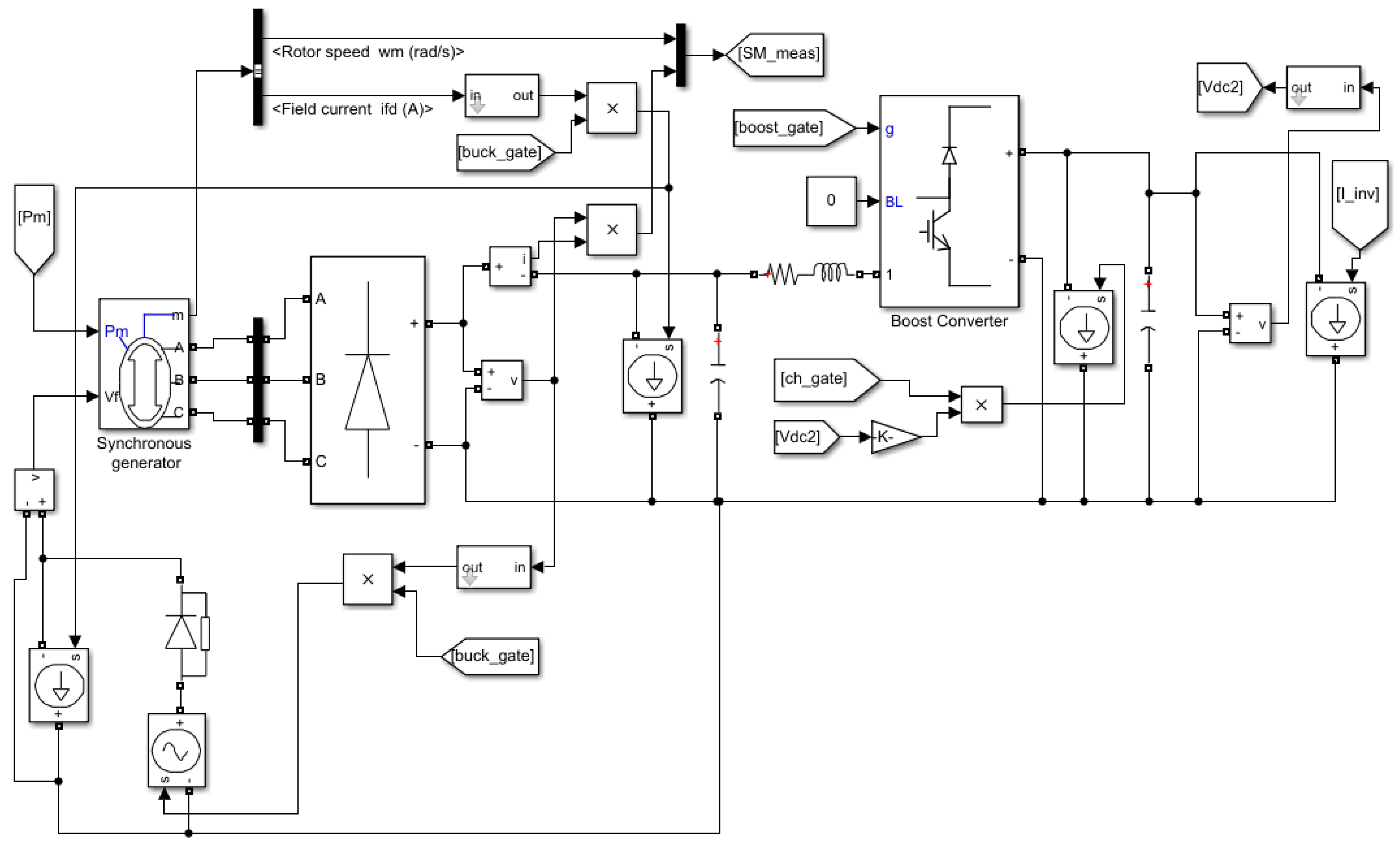
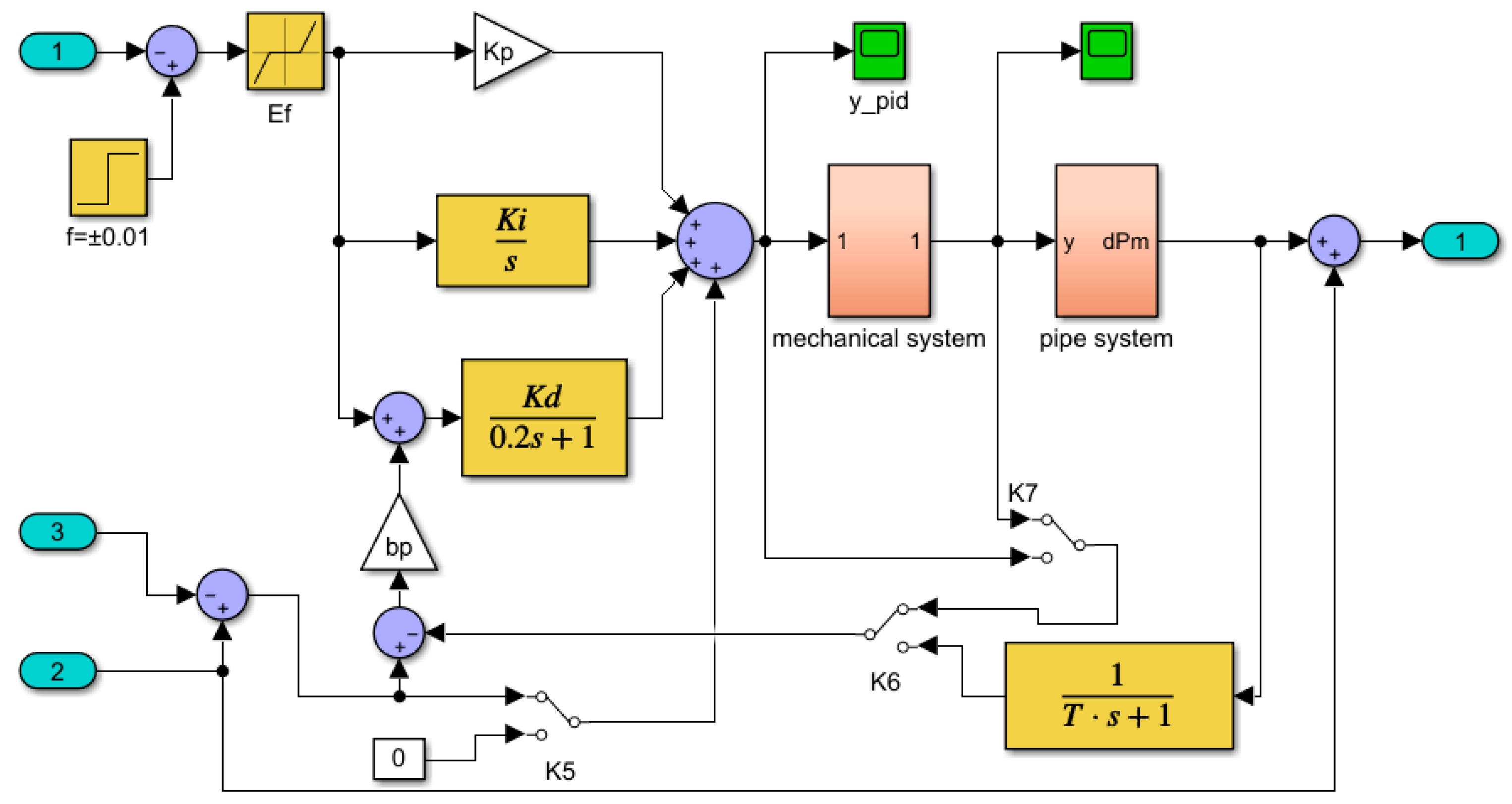
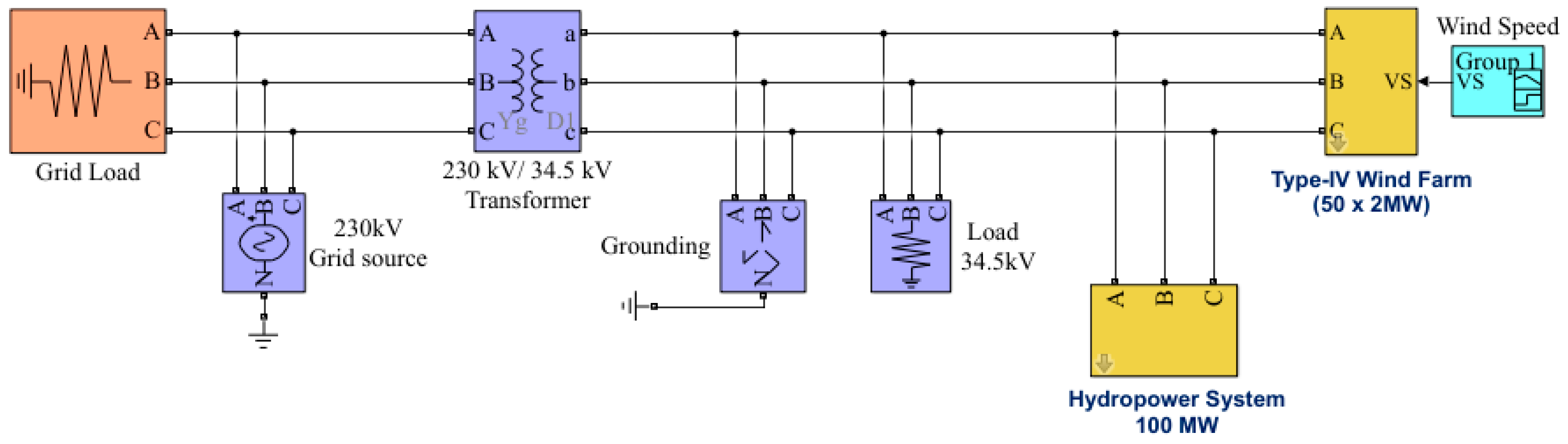
Appendix A. Block Diagram of Simulink Models

Figure A1. Block diagram of the full-size converter.
Water 16 02256 g0a1
Figure A2. Block diagram of the hydro-turbine and frequency regulation system.
Water 16 02256 g0a2
Figure A3. Model of the hybrid hydro–wind power system. The symbols A/a, B/b, and C/c represents three phases.
Water 16 02256 g0a3
The specifications of the wind turbine for the Simulink model are listed in Table A1.
Table A1. Specifications of the wind turbine.
ParameterValueParameterValue
Proportional gain of wind turbine2 puOnline impedance of device1 × 10−3 ohms
Maximum protection voltage1.25 puMaximum protection frequency1.05 pu
Minimum protection voltage0.8 puMinimum protection frequency0.95 pu
Delay time of maximum protection voltage0.1 sLower limit of power input saturation−1 pu
Delay time of minimum protection voltage5 sUpper limit of power input saturation1 pu
Snubber resistor of current source1 × 105 ohmsBoost forward voltage0 V
Snubber resistor of boost converter1 × 106 ohmsLower limit of input saturation of wind speed3 m/s
Delay time of protection frequency1 sUpper limit of input saturation of wind speed27 m/s

Appendix B. Description of the Setting of PID Control Parameter

To simplify the complexity of the calculation, the PID control parameters adopt fixed values recommended by the reference [42], including Kp = 6.433, Ki = 0.5, and Kd = 0.1. These three control parameters are always constant and do not change over time, since the hydropower system is always in the generating mode in this work. To verify the reliability of the parameter selection, a stability simulation test is conducted when the output of wind power suddenly decreases or increases at t = 10 s. The total test time is 15 s. The results in Figure A4 show that the stability responses of the hydraulic frequency fluctuate within the acceptable range of ±0.5 Hz, and they also gradually converge to zero. Therefore, the setting of the PID control parameters is reliable, since it ensures the stability of hydropower system under the influence of fluctuations in wind power.
Figure A4. Responses of the hydraulic frequency. The dotted blue lines represent the acceptable frequency range of ±0.5 Hz.
Water 16 02256 g0a4

Appendix C. Comparison of Models and Complementary Results

A comparison between the established model and the common model that generally considers the rigid-hammer effect of pipes for hydropower systems is conducted in this part. The constant wind speed is 11 m/s and the simulation time is 10 s. The corresponding complementary results based on these two models are shown in Figure A5 and Figure A6.
Figure A5. Comparative model: (a) the complementarity of output power and, (b) the fluctuation in hydraulic frequency.
Water 16 02256 g0a5
Figure A6. Model in this work: (a) the complementarity of output power and, (b) the fluctuation in hydraulic frequency.
Water 16 02256 g0a6
In Figure A5 and Figure A6, the complementarity between the hydraulic power and wind power is poor, and the corresponding hydraulic frequency exceeds the acceptable range of ±0.5 Hz for the comparative model. This is because the change rule of hydraulic power cannot be accurately simulated due to the use of rigid pipes. Conversely, the established model accurately reflects the complementarity of the output power and fluctuation in hydraulic frequency. Thus, the complementary results based on the established model are reliable.

References

  1. Routray, A.; Mistry, K.D.; Arya, S.R.; Chittibabu, B. Power output evaluation of a wind-solar farm considering the influence parameters. IET Renew. Power Gener. 2021, 15, 1613–1623. [Google Scholar] [CrossRef]
  2. Zhou, B.Z.; Lin, C.S.; Huang, X.; Zhang, H.M.; Zhao, W.H.; Zhu, S.Y.; Jin, P. Experimental study on the hydrodynamic performance of a multi-DOF WEC-type floating breakwater. Renew. Sust. Energy. Rev. 2024, 202, 114694. [Google Scholar] [CrossRef]
  3. Zhang, H.; Wu, S.; Li, H.; Zhang, J.; Zhu, C.; Zhou, H.; Jia, Y. Multi-scheme optimal operation of pumped storage wind-solar-thermal generation system based on tolerable energy abandonment. Water 2024, 16, 576. [Google Scholar] [CrossRef]
  4. Li, B.; Wang, J.; Nassani, A.A.; Binsaeed, R.H.; Li, Z. The future of Green energy: A panel study on the role of renewable resources in the transition to a Green economy. Energy Econ. 2023, 127, 107026. [Google Scholar] [CrossRef]
  5. Ju, C.; Ding, T.; Jia, W.; Mu, C.; Zhang, H.; Sun, Y. Two-stage robust unit commitment with the cascade hydropower stations retrofitted with pump stations. Appl. Energy 2023, 334, 120675. [Google Scholar] [CrossRef]
  6. Gunturu, U.B.; Hallgren, W. Asynchrony of wind and hydropower resources in Australia. Sci. Rep. 2017, 7, 8818. [Google Scholar] [CrossRef]
  7. Eising, M.; Hobbie, H.; Most, D. Future wind and solar power market values in Germany—Evidence of spatial and technological dependencies? Energy Econ. 2020, 86, 104638. [Google Scholar] [CrossRef]
  8. Guo, P.C.; Zhang, H.; Gou, D.M. Dynamic characteristics of a hydro-turbine governing system considering draft tube pressure pulsation. IET Renew. Power Gener. 2020, 14, 1210–1218. [Google Scholar] [CrossRef]
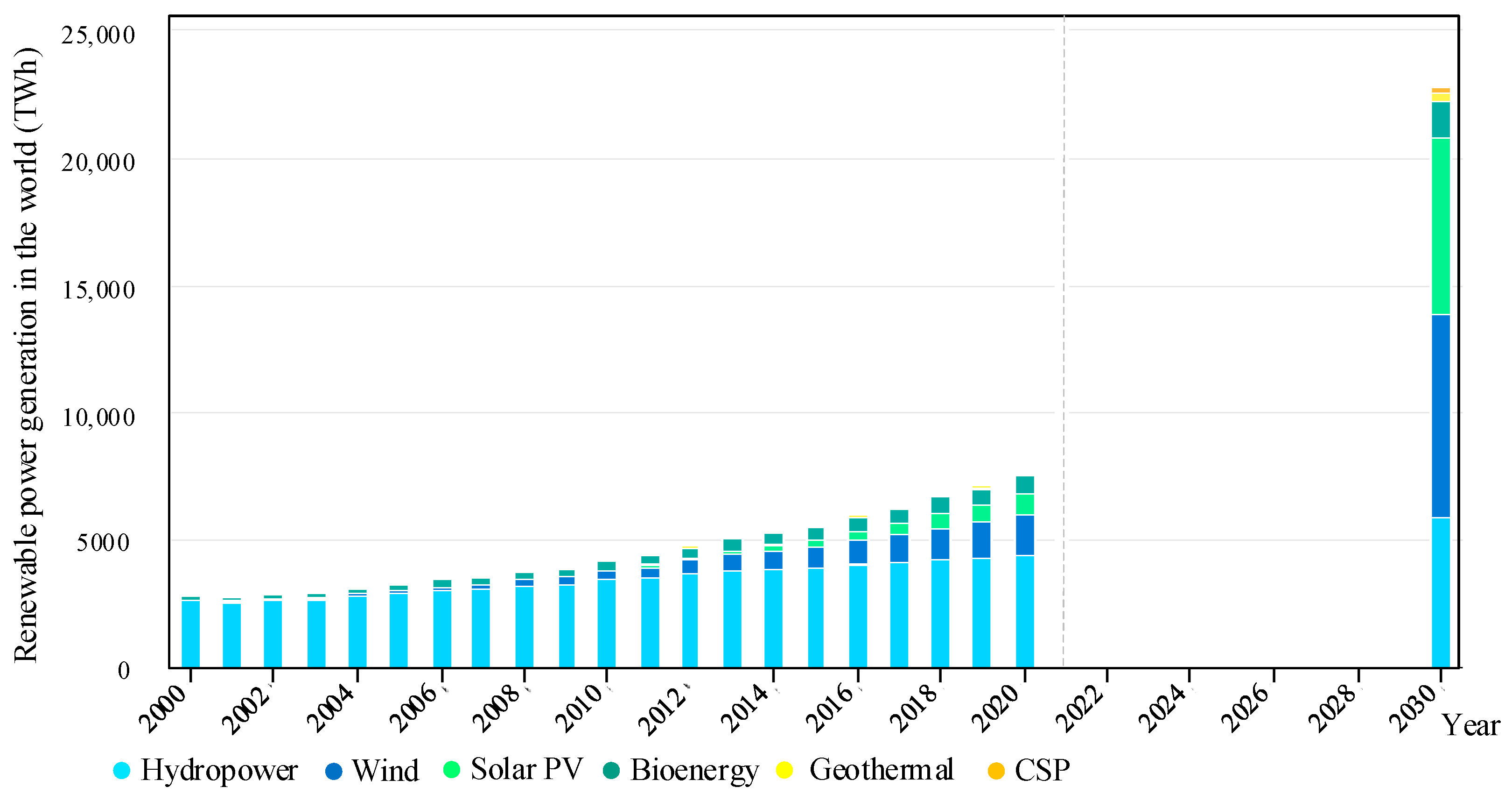
  9. IEA. Renewable Power Generation by Technology, Historic and in the Net Zero Scenario, 2000–2030; IEA: Paris, France, 2021; Available online: https://www.iea.org/data-and-statistics/charts/renewable-power-generation-by-technology-historic-and-in-the-net-zero-scenario-2000-2030 (accessed on 1 January 2023).
  10. Zhang, H.X.; Lu, Z.X.; Hu, W.; Wang, Y.T.; Dong, L.; Zhang, J.T. Coordinated optimal operation of hydro-wind-solar integrated systems. Appl. Energy 2019, 242, 883–896. [Google Scholar] [CrossRef]
  11. Ju, Y.T.; Liu, W.W.; Zhang, Z.F.; Zhang, R.S. Distributed three-phase power flow for AC/DC hybrid networked microgrids considering converter limiting constraints. IEEE Trans. Smart Grid 2022, 13, 1691–1708. [Google Scholar] [CrossRef]
  12. Simiao, M.; Ramos, H.M. Hybrid pumped hydro storage energy solutions towards wind and PV integration: Improvement on flexibility, reliability and energy costs. Water 2020, 12, 2457. [Google Scholar] [CrossRef]
  13. Mou, J.H.; Duan, P.Y.; Gao, L.; Pan, Q.K.; Gao, K.Z.; Singh, A.K. Biologically inspired machine learning-based trajectory analysis in intelligent dispatching energy storage system. IEEE Trans. Intell. Transp. Syst. 2023, 24, 4509–4518. [Google Scholar] [CrossRef]
  14. Alvarez, M.; Ronnberg, S.K.; Bermudez, J.; Zhong, J.; Bollen, M.H.J. Reservoir-type hydropower equivalent model based on a future cost piecewise approximation. Electr. Power Syst. Res. 2018, 155, 184–195. [Google Scholar] [CrossRef]
  15. Meng, Q.; Jin, X.; Luo, F.; Wang, Z.; Hussain, S. Distributionally robust scheduling for benefit allocation in regional integrated energy system with multiple stakeholders. J. Mod. Power Syst. Clean Energy 2024, 1–12. [Google Scholar] [CrossRef]
  16. Zhu, C.Y.; Wang, M.X.; Guo, M.X.; Deng, J.X.; Du, Q.P.; Wei, W.; Zhang, Y.X.; Talesh, S.S.A. Optimizing solar-driven multi-generation systems: A cascade heat recovery approach for power, cooling, and freshwater production. Appl. Therm. Eng. 2024, 240, 122214. [Google Scholar] [CrossRef]
  17. Zhu, C.Y.; Wang, M.X.; Guo, M.X.; Deng, J.X.; Du, Q.P.; Wei, W.; Zhang, Y.X.; Mohebbi, A. An innovative process design and multi-criteria study/optimization of a biomass digestion-supercritical carbon dioxide scenario toward boosting a geothermal-driven cogeneration system for power and heat. Energy 2024, 292, 130408. [Google Scholar] [CrossRef]
  18. Zhu, C.Y.; Zhang, Y.X.; Wang, M.X.; Deng, J.X.; Cai, Y.W.; Wei, W.; Guo, M.X. Optimization, validation and analyses of a hybrid PV-battery-diesel power system using enhanced electromagnetic field optimization algorithm and ε-constraint. Energy Rep. 2024, 11, 5335–5349. [Google Scholar] [CrossRef]
  19. Zhu, C.Y.; Zhang, Y.X.; Wang, M.X.; Deng, J.X.; Cai, Y.W.; Wei, W.; Guo, M.X. Simulation and comprehensive study of a new trigeneration process combined with a gas turbine cycle, involving transcritical and supercritical CO2 power cycles and Goswami cycle. J. Therm. Anal. Calorim. 2024, 149, 6361–6384. [Google Scholar] [CrossRef]
  20. Li, P.; Hu, J.P.; Qiu, L.; Zhao, Y.Y.; Ghosh, B.K. A distributed economic dispatch strategy for power-water networks. IEEE Trans. Control Netw. Syst. 2022, 9, 356–366. [Google Scholar] [CrossRef]
  21. Guo, Y.; Ming, B.; Huang, Q.; Wang, Y.M.; Zheng, X.D.; Zhang, W. Risk-averse day-ahead generation scheduling of hydro-wind-photovoltaic complementary systems considering the steady requirement of power delivery. Appl. Energy 2022, 309, 118467. [Google Scholar] [CrossRef]
  22. Majumdar, K.; Roy, P.K.; Banerjee, S. Implementation of multi-objective chaotic mayfly optimization for hydro-thermal- solar-wind scheduling based on available transfer capability problem. Int. Trans. Electr. Energy Syst. 2021, 31, e13029. [Google Scholar] [CrossRef]
  23. Wang, C.; Wang, Y.; Wang, K.S.; Dong, Y.; Yang, Y. An improved hybrid algorithm based on biogeography/complex and metropolis for many-objective optimization. Math. Probl. Eng. 2017, 2017, 2462891. [Google Scholar] [CrossRef]
  24. Zhang, Y.; Cheng, C.T.; Cao, R.; Li, G.; Shen, J.J.; Wu, X.Y. Multivariate probabilistic forecasting and its performance’s impacts on long-term dispatch of hydro-wind hybrid systems. Appl. Energy 2021, 283, 116243. [Google Scholar] [CrossRef]
  25. Shirkhani, M.; Tavoosi, J.; Danyali, S.; Sarvenoee, A.K.; Abdali, A.; Mohammadzadeh, A.; Zhang, C.W. A review on microgrid decentralized energy/voltage control structures and methods. Energy Rep. 2023, 10, 368–380. [Google Scholar] [CrossRef]
  26. Saidi, S.; Abbassi, R.; Amor, N.; Chebbi, S. Passivity-based direct power control of shunt active filter under distorted grid voltage conditions. Automatika 2016, 57, 361–371. [Google Scholar] [CrossRef]
  27. Saidi, S.; Abbassi, R.; Chebbi, S. Quality improvement of shunt active power filter with direct instantaneous power estimator based on Virtual Flux. Int. J. Control Autom. Syst. 2016, 14, 1309–1321. [Google Scholar] [CrossRef]
  28. Saidi, S.; Chebbi, S.; Jouini, H. Harmonic and reactive power compensations by shunt active filter controlled by adaptive fuzzy logic. Int. Rev. Model. Simul. 2011, 4, 1487–1492. [Google Scholar]
  29. Avila, L.; Mine, M.R.M.; Kaviski, E.; Detzel, D.H.M. Evaluation of hydro-wind complementarity in the medium-term planning of electrical power systems by joint simulation of periodic stream fl ow and wind speed time series: A Brazilian case study. Renew. Energy 2021, 167, 685–699. [Google Scholar] [CrossRef]
  30. Liu, S.; Han, W.Z.; Zhang, Z.; Chan, F.T.S. An analysis of performance, pricing, and coordination in a supply chain with cloud services: The impact of data security. Comput. Ind. Eng. 2024, 192, 110237. [Google Scholar] [CrossRef]
  31. Fayek, H.H.; Kotsampopoulos, P. Central tunicate swarm NFOPID-based load frequency control of the Egyptian power system considering new uncontrolled wind and photovoltaic farms. Energies 2021, 14, 3604. [Google Scholar] [CrossRef]
  32. Ren, Y.; Yao, X.H.; Liu, D.; Qiao, R.Y.; Zhang, L.L.; Zhang, K.; Jin, K.Y.; Li, H.W.; Ran, Y.L.; Li, F. Optimal design of hydro-wind-PV multi-energy complementary systems considering smooth power output. Sustain. Energy Technol. Assess. 2022, 50, 101832. [Google Scholar] [CrossRef]
  33. Tang, Y.J.; Fang, G.H.; Tan, Q.F.; Wen, X.; Lei, X.H.; Ding, Z.Y. Optimizing the sizes of wind and photovoltaic power plants integrated into a hydropower station based on power output complementarity. Energy Conv. Manag. 2020, 206, 112465. [Google Scholar] [CrossRef]
  34. Li, H.H.; Mahmud, M.A.; Arzaghi, E.; Abbassi, R.; Chen, D.Y.; Xu, B.B. Assessments of economic benefits for hydro-wind power systems: Development of advanced model and quantitative method for reducing the power wastage. J. Clean Prod. 2020, 277, 123823. [Google Scholar] [CrossRef]
  35. Karaagac, U.; Mahseredjian, J.; Gagnon, R.; Gras, H.; Saad, H.; Cai, L.J.; Kocar, I.; Haddadi, A.; Farantatos, E.; Bu, S.Q.; et al. A generic EMT-type model for wind parks with permanent magnet synchronous generator full size converter wind turbines. IEEE Power Energy Technol. Syst. J. 2020, 6, 131–141. [Google Scholar] [CrossRef]
  36. Gao, D.W.; Wu, Z.P.; Yan, W.H.; Zhang, H.G.; Yan, S.J.; Wang, X. Comprehensive frequency regulation scheme for permanent magnet synchronous generator-based wind turbine generation system. IET Renew. Power Gener. 2019, 13, 234–244. [Google Scholar] [CrossRef]
  37. Li, J.; Wang, N.; Zhou, D.; Hu, W.H.; Huang, Q.; Chen, Z.; Blaabjerg, F. Optimal reactive power dispatch of permanent magnet synchronous generator-based wind farm considering levelised production cost minimization. Renew. Energy 2020, 145, 1–12. [Google Scholar] [CrossRef]
  38. Banu, J.B.; Moses, M.B.; Ganapathy, S. Maximum Power Point Tracking of Direct-Drive PMSG with High-Efficiency Boost Converter. In Proceedings of the International Conference on Emerging Trends and Advances in Electrical Engineering and Renewable Energy (ETAEERE), Munich, Germany, 26–27 September 2018. [Google Scholar] [CrossRef]
  39. Soufyane, B.; Abdelhamid, R.; Smail, Z.; Elhafyani, M.L.; El Hajjaji, A. Fully Robust Sensorless Control of Direct-Drive PMSG Wind Turbine Feeding a Water Pumping System. Fully Robust Sensorless Control of Direct-Drive PMSG Wind Turbine Feeding a Water Pumping System. IFAC-PapersOnLine 2020, 53, 12797–12802. [Google Scholar] [CrossRef]
  40. Trevisan, A.S. Type-IV Wind Turbine. MATLAB Central File Exchange. 2022. Available online: https://www.mathworks.com/matlabcentral/fileexchange/71235-type-iv-wind-turbine (accessed on 1 December 2023).
  41. Trevisan, A.S.; El-Deib, A.A.; Gagnon, R.; Mahseredjian, J.; Fecteau, M. Field Validated Generic EMT-Type Model of a Full Converter Wind Turbine Based on a Gearless Externally Excited Synchronous Generator. IEEE Trans. Power Deliv. 2018, 33, 2284–2293. [Google Scholar] [CrossRef]
  42. Ling, D.J. Bifurcation and Chaos of Hydraulic Turbine Governor. Ph.D. Thesis, Hohai University, Nanjing, China, 2007. Available online: http://www.wanfangdata.com.cn/details/detail.do?_type=degree&id=Y1241732 (accessed on 1 December 2023).
  43. Cheng, C.T.; Wu, H.J.; Wu, X.Y.; Shen, J.J.; Wang, J. Power generation scheduling for integrated large and small hydropower plant systems in southwest China. J. Water Resour. Plan. Manag. ASCE 2017, 143, 04017027. [Google Scholar] [CrossRef]
  44. Wang, P.F.; Deng, Y.W.; Li, H.N.; Chen, D.Y. Making connections: Information transfer in hydropower generation system during the transient process of load rejection. Sustain. Energy Technol. Assess. 2022, 50, 101766. [Google Scholar] [CrossRef]
  45. Zeng, Y.; Qian, J.; Guo, Y.K.; Yu, S.G. Differential equation model of single penstock multi-machine system with hydraulic coupling. IET Renew. Power Gener. 2019, 13, 1153–1159. [Google Scholar] [CrossRef]
  46. Li, H.H.; Zhang, R.F.; Mahmud, A.M.; Hredzak, B. A novel coordinated optimization strategy for high utilization of renewable energy sources and reduction of coal costs and emissions in hybrid hydro-thermal-wind power systems. Appl. Energy 2022, 320, 119019. [Google Scholar] [CrossRef]
  47. Wang, J.Z.; Qin, S.S.; Zhou, Q.P.; Jiang, H.Y. Medium-term wind speeds forecasting utilizing hybrid models for three different sites in Xinjiang, China. Renew. Energy 2015, 76, 91–101. [Google Scholar] [CrossRef]
  48. Qawaqzeh, M.Z.; Szafraniec, A.; Halko, S.; Miroshnyk, O.; Zharkov, A. Modelling of a household electricity supply system based on a wind power plant. Prz. Elektrotech. 2020, 96, 36–40. [Google Scholar] [CrossRef]
  49. Wu, Y.Y.; Li, Q.L.; Li, G.X.; He, B.; Dong, L.; Lang, H.N.; Zhang, L.J.; Chen, S.P.; Tang, X.X. Vertical wind speed variation in a metropolitan city in South China. Earth Space Sci. 2022, 9, e2021EA002095. [Google Scholar] [CrossRef]
  50. Basker, I.; Venkatesan, M.N. 3D-CFD flow driven performance analysis of new non-cylindrical helical vertical axis wind turbine for fluctuating urban wind conditions. Energy Sources Part A-Recovery Util. Environ. Eff. 2022, 44, 2186–2207. [Google Scholar] [CrossRef]
  51. Xu, B.B.; Li, H.H.; Campana, P.E.; Hredzak, B.; Chen, D.Y. Dynamic regulation reliability of a pumped-storage power generating system: Effects of wind power injection. Energy Conv. Manag. 2020, 222, 113226. [Google Scholar] [CrossRef]
  52. Abbassi, R.; Saidi, S.; Urooj, S.; Alhasnawi, B.N.; Alawad, M.A.; Premkumar, M. An Accurate Metaheuristic Mountain Gazelle Optimizer for Parameter Estimation of Single- and Double-Diode Photovoltaic Cell Models. Mathematics 2023, 11, 4565. [Google Scholar] [CrossRef]
Figure 1. The huge development potential for hydropower and wind power generation: an upward tendency over the world to 2030. The capacity of hydropower generation will increase by half, to about 6000 TWh relative to the 2020 level. The capacity of wind power generation will quadruple to 14,000 TWh compared with the 2000 level. Such growth trends are much higher than other renewable energy sources like solar power and bioenergy.
Water 16 02256 g001
Figure 2. Integration of hydropower and wind power systems.
Water 16 02256 g002
Figure 3. The curve of wind power coefficient Cp.
Water 16 02256 g003
Figure 4. Optimization framework of this paper.
Water 16 02256 g004
Figure 5. Wind speed, power output, and power structure in Scenario 1. (a) Scenario 1: complementary characteristic of the hydro–wind power system under the constant (Type 1), mutational (Type 2), and random (Type 3) wind speeds. (b) Scenario 1: power structure of hybrid hydro–wind system. Figure 5b is a larger version of the red dashed area in Figure 5a.
Water 16 02256 g005
Figure 6. End-use power, mix-produced power, and power loss in Scenario 1. (a) Scenario 1: end-use power of grid and mix-produced power of hybrid system under the constant (Type 1), mutational (Type 2), and random (Type 3) wind speeds. (b) Scenario 1: transmission power loss under the constant (Type 1), mutational (Type 2), and random (Type 3) wind speeds.
Water 16 02256 g006
Figure 7. Hydraulic tracing effect and power loss in Scenario 2. (a) Scenario 2: hydraulic tracing effect of the hydro–wind power system under the constant (Type 1), mutational (Type 2), and random (Type 3) wind speeds. (b) Scenario 2: power loss under different wind speeds.
Water 16 02256 g007aWater 16 02256 g007b
Figure 8. Effect of WTs’ number on hydraulic suppression effect under Type 2 wind. (a) Power complementarity and fluctuation in hydraulic frequency. (b) Out-of-control hydraulic frequency.
Water 16 02256 g008
Figure 9. Effect of capacity allocation on power loss under Type 2 wind.
Water 16 02256 g009
Table 1. The summary of literature review for achieving the optimal coordinated operation.
SummaryClassification of Optimization Ways
Way 1Way 2Way 3
DescriptionEstablish an optimization model to optimize the operating coefficients.Design an operational optimization method or scheduling method to maximize the benefits of operation goals.Optimize the complementary performance of the fluctuations in output power or frequency.
Common characteristicThe calculation process is reasonable and the optimization results are reliable.
Differences(i) Key stepEstablish a model that reflects the coupling characteristics of each component or subsystem.Present a linear/nonlinear programming method.Emphasize in-depth excavation from a certain research perspective.
(ii) Key factor that is related to the reliability of resultsModel outputs.Objective functions and constraints.Controllers, operation variables, or operation scenarios.
(iii) The literature involvedReferences [10,11,12,13,14]References [15,16,17,18,19,20,21,22,23,24]References [25,26,27,28,29,30,31,32,33]
Table 2. Descriptions of complementary indicators in the optimization methodology.
IndicatorDefinition
  • Hydraulic tracing power
  • This is equal to the power load minus the actual hydraulic power. The coordinated operating quality of the hybrid system is excellent when the hydraulic tracing power is closer to the actual wind power.
b.
Volatility of wind power
  • This is equal to the difference between the maximum and minimum actual wind power.
c.
Volatility of hydraulic frequency
  • This is equal to the ratio of the product of the hydro-turbine rotational speed and generator pole number to 60, which is generally revealed by the value and occurrence time of the maximum deviation. The hydraulic frequency cannot exceed ± 0.5 Hz, which is an accepted range for the stability of power grids.
d.
Power loss
  • This is equal to the difference between the end-use power of a grid and the mix-produced power of a hybrid system, which is generally revealed by the mean, maximum, and peak time.
Table 3. Descriptions of the studied two scenarios.
ScenarioCharacteristics
Scenario 1: on-demand hydropower scenarioThe planned power generation is equivalent to the load demand.
The installed hydropower capacity that can participate in regulation is prone to shortages if there is a prolonged period of extreme wind speed.
It is not easy to produce surplus water for the hydropower system.
Scenario 2: surplus hydropower scenarioThe planned power generation is larger than the load demand.
When the fluctuation in wind power is large, the installed hydropower capacity that can participate in regulation is sufficient.
More surplus water is produced.
Table 4. Optimization results of the capacity allocation under the constant (Type 1), mutational (Type 2), and random (Type 3) wind speeds.
Wind TypeWT NumberWind Capacity (MW)Complementary CharacteristicHydraulic FrequencyPower Loss
Wind Volatility (p.u.)Hydraulic Tracing EffectMaximum Deviation (Hz)Occurrence Time (s)Mean (MW)Maximum (MW)Peak Time (s)
1511020.0121Excellent0.1235.176.82 7.00 0.95
751500.0174Excellent0.1981.459.00 10.79 0.6
1002000.0244Good0.26864.9311.80 14.80 0.62
1252500.0297Good0.30954.10 15.50 19.00 0.8
1503000.0379Good0.4321.1219.00 24.00 0.76
1633260.0413Good0.42971.3821.80 27.50 0.79
164328------0------
2511020.6352Excellent0.077623.566.90 7.50 0.47
551100.686Excellent0.095726.767.20 7.75 0.46
601200.7505Good0.356827.647.75 8.80 0.47
61122------21.55------
3511020.1397Excellent0.23291.60 6.86 7.43 0.46
751500.208Good0.321915.989.38 11.21 0.49
1002000.2744Good0.47612.6213.50 16.56 0.49
1252500.3427Good0.5000 2.3119.50 23.91 0.57
127254--------------
Disclaimer/Publisher’s Note: The statements, opinions and data contained in all publications are solely those of the individual author(s) and contributor(s) and not of MDPI and/or the editor(s). MDPI and/or the editor(s) disclaim responsibility for any injury to people or property resulting from any ideas, methods, instructions or products referred to in the content.

