Application of HKELM Model Based on Improved Seahorse Optimizer in Reservoir Dissolved Oxygen Prediction

Abstract

As an important part of environmental science and water resources management, water quality prediction is of great importance. In order to improve the efficiency and accuracy of predicting dissolved oxygen (DO) at the outlet of a reservoir, this paper proposes an improved Seahorse Optimizer to enhance the hybrid kernel extreme learning machine model for water quality prediction. Firstly, the circle chaotic map is used to initialize the hippocampus population to improve the diversity and quality of the population, and then the sine and cosine strategy is used to replace the predation behavior of the hippocampus to improve the global search ability. Finally, the lens imaging reverse learning strategy is used to expand the search range and prevent it from falling into the local optimal solution. By introducing two kernel functions, a global kernel function (Poly) and a local kernel function (RBF), a new hybrid kernel function extreme learning machine is formed by linearly combining these two kernel functions. The parameters of this HKELM are optimized with the improved Seahorse Optimizer, and the water quality prediction model of CZTSHO-HKELM is constructed. The simulation results show that the operating efficiency and prediction accuracy of the model are better than those of the ELM, CZTSHO-ELM, CZTSHO-KELM, and SHO-HKELM models, with the correlation coefficients increased by 5.5%, 3.3%, 3.4%, and 7.4%, respectively. The dissolved oxygen prediction curve is close to the actual dissolved oxygen change, which can better meet the requirements of reservoir water quality prediction. The above method can be applied to further accurately predict the water quality of the reservoir.

1. Introduction

With the rapid development of the social economy and the acceleration of industrialization, water pollution has become one of the important environmental problems faced by all countries in the world. As an indispensable material basis for the production and life of human society, the quality of water resources is directly related to our living conditions and living environment. An effective water quality prediction method is not only a necessary condition for the protection of water resources, but also plays an indispensable role in ecological security, public health, economic development, and the water cycle [1].

The water quality directly reflects the health status of a water body, and efficient and accurate water quality prediction can effectively monitor the status of a water body and its changing trend. Real-time monitoring can detect current water quality conditions, but it cannot predict future changes in advance. Water quality forecasting can provide early warning of possible pollution events based on historical data and trend analysis, giving managers time to take preventive and response measures to avoid the harm caused by water quality deterioration [2]. For example, through real-time monitoring and predicting of reservoir water quality, we can take steps to reduce the spread of pollution at an early stage, protect aquatic ecosystems, and ensure the sustainable use of water resources [3]. Therefore, the development and application of advanced water quality prediction technologies, such as real-time prediction models, is of great significance in coping with the increasingly severe challenges of the water environment. These technologies can process complex water quality data, predict water quality changes, and provide a scientific basis for water resource management and environmental protection. As conducted by Jenifel G M (2024), the research on a secure water quality prediction system using machine learning and blockchain technologies demonstrates the potential of these advanced methods [4]. Among them, dissolved oxygen (DO) is an important index to measure the degree of water pollution, and the monitored water quality data are time-varying and nonlinear. Therefore, how to use these data to accurately predict the change trend of dissolved oxygen and future water quality and make reasonable decisions in a timely manner has become a hot spot in contemporary research.

Common water quality prediction methods include artificial neural networks (ANNs), regression analysis (RA), and support vector regression (SVR) [5,6,7]. A new comprehensive deep learning water quality prediction algorithm is proposed by Yan J Z et al., which uses various methods to clean and preprocess water quality data, and then uses a one-dimensional residual convolution neural network and a two-way gated cycle unit to extract water quality parameters [8]. Huang, G et al. put forward a new learning algorithm called the extreme learning machine for the first time, which is thousands-of-times faster than the traditional popular feedforward neural network learning algorithm [9]. Jagadeesh, A et al. compared the extreme learning machine (ELM) with different algorithms in upstream water quality prediction, laying a foundation for water quality prediction research [10]. Javad, A et al. predicted the real-time chemical oxygen demand (COD) value by combining a kernel-based extreme learning machine with an intelligent optimization algorithm [11].

The above methods have obtained a lot of research results for the prediction of DO concentration. However, DO concentration is affected by a variety of water quality parameters, and the parameters show complex nonlinear and correlation characteristics, which has a great impact on the prediction of DO [12,13]. As an interdisciplinary subject, water quality prediction involves knowledge and technology in many fields such as environmental science, computer science, and statistics. This paper not only aims to propose a new prediction method but also hopes to provide theoretical and practical experience for researchers and practitioners in the field of water quality monitoring and prediction through in-depth research and analysis. Therefore, how to use ELM and intelligent optimization algorithms to improve the accuracy and reliability of water quality prediction is discussed. However, there are some problems in the actual prediction process of the ELM, such as unstable model prediction effects and an inability to fully reveal sample information. When the number of hidden layers is too large, it will lead to overfitting. The characteristics of high correlation among water quality indexes are ignored. Using multivariate correlation and time series data of water quality, it is proposed to introduce a global kernel function and a local kernel function into the ELM via linear combination to yield an HKELM. Then, the SHO intelligent optimization algorithm is improved with three improvement measures. Finally, the improved Seahorse Optimizer (SHO) is used to optimize each hyperparameter of the HKELM, so as to optimize the network structure of the mixed kernel extreme learning machine and obtain better prediction results.

2. Materials and Methods

2.1. Seahorse Optimization Algorithm

2.1.1. SHO

The Seahorse Optimizer (SHO) is a population-based optimization algorithm proposed in 2022 [14], which mainly includes the initialization, movement, predation, and reproduction behaviors of seahorse populations.

(1)

initialize

The population initialization of the SHO algorithm is the same as most intelligent evolutionary optimization algorithms, assuming that each seahorse represents a candidate solution to the problem search space, and each solution $X_i$ is randomly generated between the lower bound $B_{LB}$ and the upper bound $B_{UB}$ of a particular problem:

$$X_i=\left[x_i^1,\cdots ,x_i^{D_{im}}\right]$$

(1)

$$X_i^j=f_r\left(B_{UB}^j-B_{LB}^j\right)+B_{LB}^j$$

(2)

where $X_i$ represents the $i$ th solution; $D_{im}$ is the dimension of the solution space; and $X_i^j$ represents the solution of the $j$th dimension of individual $i$. $f_r$ represents the random number between $\left[0, 1\right]$; $i$ is the positive integer between $\left[1,n_{pop}\right]$ and $j$ is the positive integer between $[1,D_{im}]$, where $n_{pop}$ is the number of individuals.

(2)

Motor behavior of the hippocampus

In motion behavior, the movement of an individual hippocampus is divided into two cases: global search in the search space and local search near the possible optimal position. In order to distinguish the performance of the algorithm, a random number $R_1$ with normal distribution is set.

When $R_1>0$, the hippocampal individual moves with the ocean vortex to conduct a local search, and the position update expression is as follows:

$$X_{new}^1\left(t+1\right)=X_i\left(t\right)+Levy\left(\lambda \right)\left(\left(X_{elite}\left(t\right)-X_i\left(t\right)\right)\times x\times y\times z+X_{elite}\left(t\right)\right)$$

(3)

where $Levy\left(\lambda \right)$ is the flight distribution function, $X \left(t\right)$ represents the elite matrix in the population, and $x, y, z$ represent the three-dimensional components of the spiral motion, where $x=\rho \times cos\theta$.

When $R_1\le 0$, the hippocampal individual conducts Brownian motion within the ocean and carries out a global search, and the position update expression is as follows:

$$X_{new}^1\left(t+1\right)=X_i\left(t\right)+rand\times l\times {\beta }_t\times \left(X_i\left(t\right)-{\beta }_t\times X_{elite}\right)$$

(4)

where $l$ is the constant coefficient, and ${\beta }_t$ is the random walk coefficient on $\left(pop,Dim\right)$, which follows the standard normal distribution.

(3)

Predatory behavior of seahorses

The probability of successful predation of a hippocampus is greater than 90%, so the random number $R_2$ is designed to distinguish between success and failure. When $R_2>0.1$, it indicates successful predation of hippocampus. At this time, the new position of hippocampus after iteration $t$ is as follows:

$$X_{new}^2\left(t+1\right)=\sigma \left(Elite\left(t\right)-rand\times X_{new}^1\left(t\right)\right)+\left(\left(1-\sigma \right)\times Elite\left(t\right)\right)$$

(5)

When $R2\le 0.1$, it indicates that hippocampal predation fails, and the hippocampus tends to explore space and conduct a global search:

$$X_{new}^2\left(t+1\right)=\left(1-\sigma \right)\times \left(X_{new}^1\left(t\right)-rand\times Elite\left(t\right)\right)+\left(\sigma \times X_{new}^1\left(t\right)\right)$$

(6)

where $X_{new}^2(t+1)$ represents the new position of the seahorse after it moves at iteration $t$, $r_2$ is the random number between $[0, 1]$, and the weight $\sigma$ of the influence factor is adjusted to linearly decrease; the formula is as follows:

$$\sigma ={\left(1-{\displaystyle \frac{t}{max\text{\_}iter}}\right)}^{{\displaystyle \frac{2t}{max\text{\_}iter}}}$$

(7)

where $max\text{\_}iter$ is the maximum number of iterations.

(4)

The reproductive behavior of seahorses

According to the fitness value, the population is divided into male and female groups, but the hippocampus is special because the male gives birth to the next generation, so the SHO algorithm selects half of the individuals with the best fitness as the father $F_x$, and the other half as the mother $M_x$:

$$F_x=X_{sort}^2\left(1\text{:}{\displaystyle \frac{n_{pop}}{2}}\right)$$

(8)

$$M_x=X_{sort}^2\left({\displaystyle \frac{n_{pop}}{2}}+1\text{:}{n}_{pop}\right)$$

(9)

The $X_{sort}^2$ in the formula means that all $X_{new}^2$ are arranged in ascending order of fitness values, and random mating produces an offspring hippocampal individual with the following expression:

$$h_i=r_3{F}_{x,i}+\left(1-r_3\right)M_{x,i}$$

(10)

In the formula, $r_3$ is the random number between $[0, 1]$; $i$ is a positive integer in the range of $[1, n_{pop}/2]$. The offspring generated through breeding behavior are sorted again with fitness values according to the original set population size, and the top hippocampal individuals are selected to form a new population to participate in the next iteration.

2.1.2. Improved Seahorse Optimizer

Although the original algorithm performs well in certain scenarios, it still has some limitations when facing more complex water quality datasets. Therefore, we have made three improvements to the original algorithm as follows.

(1)

Circle chaotic mapping

Population initialization is a key step in many optimization algorithms because it can have a significant impact on the performance of the algorithm. The location of the initial hippocampal individuals randomly generated via the SHO may lead to uneven coverage of the search space, resulting in a significant reduction in population diversity and population quality, and the algorithm space is not fully covered, thus affecting the convergence speed and solution accuracy. Chaotic mapping has the characteristics of ergodicity, nonlinearity, and randomness, so it is a common method to solve this problem, so chaotic initialization is introduced, which can increase the randomness of search and help to explore the search space more comprehensively [15]. At present, there are many different chaotic maps in the field of optimization algorithms. Djamel, H et al. [16] proposed an enhanced logistic chaotic map, and Zhiwen, G et al. [17] constructed a hybrid optimization algorithm with a Tent map, but most of them have the problems of limited range of system parameters and uneven distribution of chaotic sequences. As a result, the chaos efficiency is low, while the circle chaotic map is stable and has high coverage, so this paper adopts the circle chaotic map to generate the initial group, which is defined as follows:

$$X_{i+1}=mod\left({AX}_i+B-\left({\displaystyle \frac{C}{A\pi }}\right)\sin \left(E\pi X_i\right),1\right)$$

(11)

where $i$ is the dimension of the solution, and $A,B, \mathrm{a}\mathrm{n}\mathrm{d} C$ are constants, and their values can be adjusted to change the effect of the chaotic mapping. In this paper, $A=1,B=0.3, \mathrm{a}\mathrm{n}\mathrm{d} C=0.3$ are used, so the algorithm exhibits a better optimization effect and high ergodic property. When $i=3000$, the dimension distribution and histogram effects of the initial solution are shown in Figure 1.

Circle chaotic mapping was used to generate the initial population. Compared with the randomly distributed population, the initial location distribution of the improved population was more uniform, which improved the ergodicity and uniformity of the initial hippocampal individual in the search space, increased the diversity of the population location, and improved the defect that the Seahorse Optimizer, due to its own limitations, was prone to fall into local extreme values, thus improving the optimization efficiency of the algorithm.

(2)

Sine–cosine strategy replaces hippocampal predation

In the process of hippocampal predation, the location of the food source plays a very important role, affecting the direction of the whole hippocampal population. Standard SHO uses a random number $R_2$ to distinguish the two results of predation. When the predation is successful, the hippocampal individual is closer to the elite individual, and if the predation fails, the algorithm switches to a global search. When the hippocampal individual engages in predation, there is a high probability that it is already near the elite individual. This will not only aggravate the situation of the algorithm falling into the local extreme value but will also consume more time in behavior that is not helpful to the algorithm’s optimization. When the food that is sought is located in the local optimal, a large number of followers will swarm into the place, and the whole group will be stagnant at this time, resulting in the loss of population location diversity. In this paper, a sine–cosine algorithm [18] (SCA) was adopted in the position update of the discoverer in the seahorse search algorithm, and this periodic change was introduced into the search process by using the oscillatory change characteristics of sine and cosine functions. This helps keep the search individual diverse. The goal of SCA is to find the optimal solution at the global and local scales, and by combining the sine and cosine models, it can be more flexible to adapt to different types of optimization problems, thereby improving the ability of a global search.

The value $r_1=a-at/Max\text{\_}iter$ (where $a$ is a constant and $t$ is the number of iterations) of the step size search factor of the sine–cosine algorithm is linearly decreasing with the iterative process of the SHO algorithm, which is not conducive to balancing the global and local development capabilities of SHO. Inspired by the search mechanism and the position update formula in the Seahorse Optimizer, replace the predation behavior in the SHO with the sine and cosine terms in SCA when:

$$r_1^{\prime }=a\times {\left(1-{\left({\displaystyle \frac{t}{Max\text{\_}iter}}\right)}^{\eta }\right)a}^{{\displaystyle \frac{1}{\eta }}}$$

(12)

In the formula, $\eta$ is the adjustment coefficient, which is set as $\eta =1.2$, and $a=1$ in this paper.

In the whole search process of the SHO algorithm, the position of new population individuals is often affected by the current position, so a nonlinear weight factor is introduced to adjust the dependence of the population’s individual position update on hippocampal individuals at this time; the formula is as follows:

$$\omega ={\displaystyle \frac{e^{\frac{t}{Max\text{\_}iter}}-1}{e-1}}$$

(13)

At the initial stage of optimization, a smaller $\omega$ can reduce the impact of an individual position update on the current position and improve the global optimization ability. With the increase of iterations, a larger $\omega$ in the later stage makes use of the high dependence of the current position information and individual position update to accelerate the convergence speed, and a new formula for the discoverer position update is obtained as follows:

$$Sea\text{\_}horses\text{\_}new2=\omega \times X_{i,j}^t+r_1^{\prime }\times \sin r_2\times \left|r_3\times X_{elite}-X_{i,j}^t\right|,R2<ST$$

(14)

$$Sea\text{\_}horses\text{\_}new2=\omega \times X_{i,j}^t+r_1^{\prime }\times \sin r_2\times \left|r_3\times X_{elite}-X_{i,j}^t\right|,R2\ge ST$$

(15)

Among them, $r_2$ and $r_3$ are random numbers between $0$ and $2\pi$, $r_2$ determines the movement range of the hippocampus, and $r_3$ controls the influence of the optimal individual on the next position of the hippocampus.

(3)

Lens imaging reverse learning strategy

Reverse learning is an improved strategy to calculate the reverse solution of the current location and thus expand the search scope. Using the reverse learning strategy after hippocampal progeny can improve the optimization ability of the algorithm. However, the reverse solution obtained by reverse learning is fixed. If the hippocampus individual has fallen into the local optimal and the reverse solution is worse than the current solution, it cannot be made to jump out of the local optimal. Reverse learning in lens imaging [19] can solve this problem, and the reverse learning strategy in lens imaging is shown in Figure 2:

In two-dimensional space, the interval on the axis $[LB,UB]$ is the search range of the solution, the Y-axis represents a convex lens with a focal length of $r$, and there is an object $Q$ on the X-axis with a height of $h$ and a projection $x$ on the X-axis. By presenting the inverted real image $Q^{*}$ on the other side of the convex lens, the height is $h^{*}$, and the projection on the X-axis is $x^{*}$; it can be deduced that

$${\displaystyle \frac{\frac{LB+UB}{2}-x}{x^{*}-\frac{LB+UB}{2}}}={\displaystyle \frac{h}{h^{*}}}$$

(16)

Let $K=h/h^{*}$ be the regulatory factor and rewrite the above formula to obtain the reverse point $x^{*}$, which is the formula for calculating the position of the hippocampal breeding offspring:

$$Sea\text{\_}horse\text{\_}offspring={\displaystyle \frac{UB+LB}{2}}+{\displaystyle \frac{UB+LB}{2k}}-{\displaystyle \frac{x}{k}}$$

(17)

When $K=1$, it is the reverse learning solution formula. By adjusting the size of $k$, a dynamically changing reverse solution can be obtained in the lens imaging reverse learning, and its small change will significantly change the search range, thereby improving the search capability of SHO. In this paper, the following is adopted:

$$k={\left(1+{\left({\displaystyle \frac{t}{Max\text{\_}iter}}\right)}^2\right)}^{14}$$

(18)

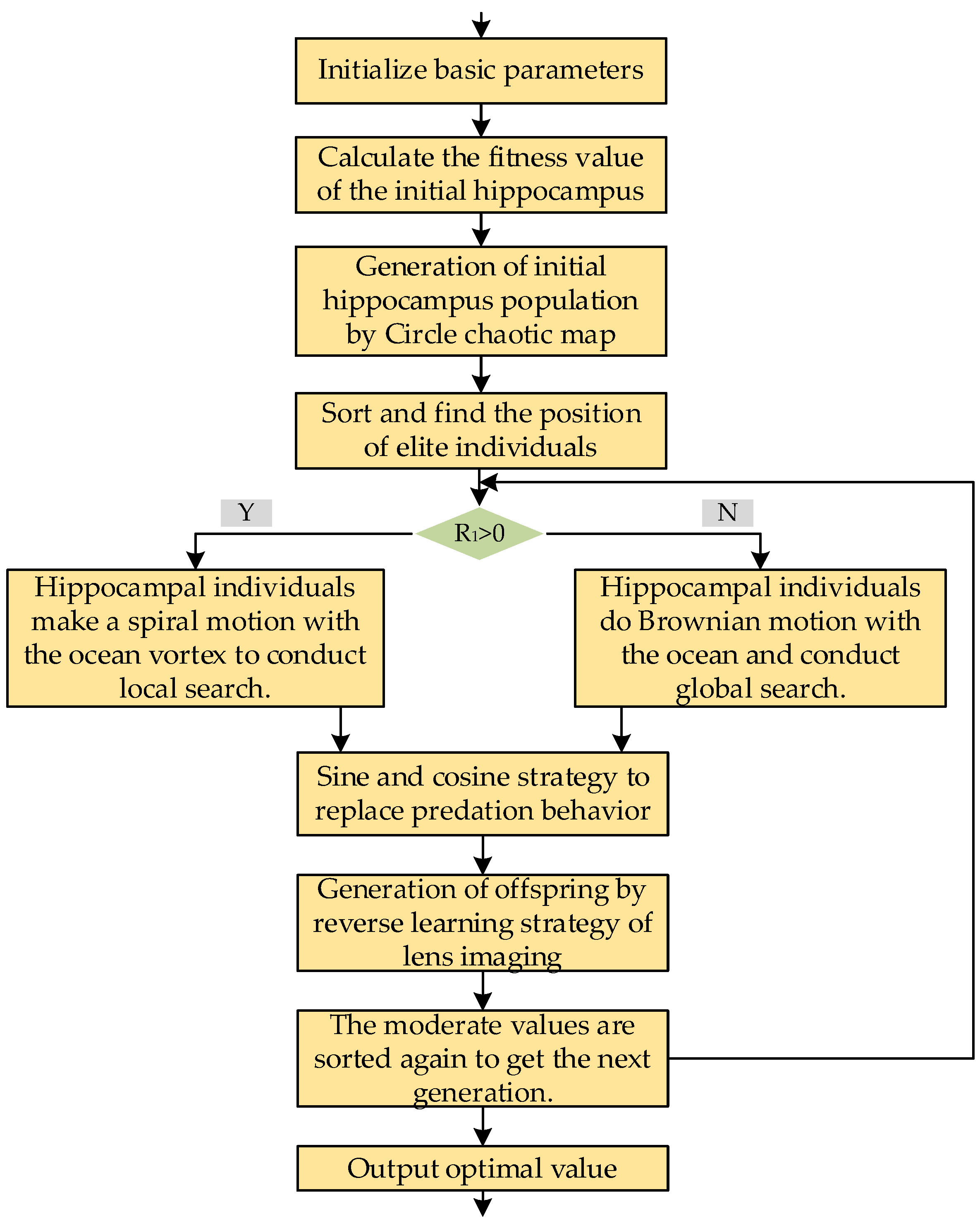
2.1.3. Improve the Implementation Steps of Seahorse Algorithm

Circle chaotic mapping, sine–cosine strategy and lens imaging reverse learning were used to improve the original Seahorse Optimizer and calculate the initial hippocampal fitness value. The improved flow chart is shown in Figure 3. The pseudo-code for the improved Seahorse Optimizer is provided in Appendix A at the end of this article.

2.2. Performance Test

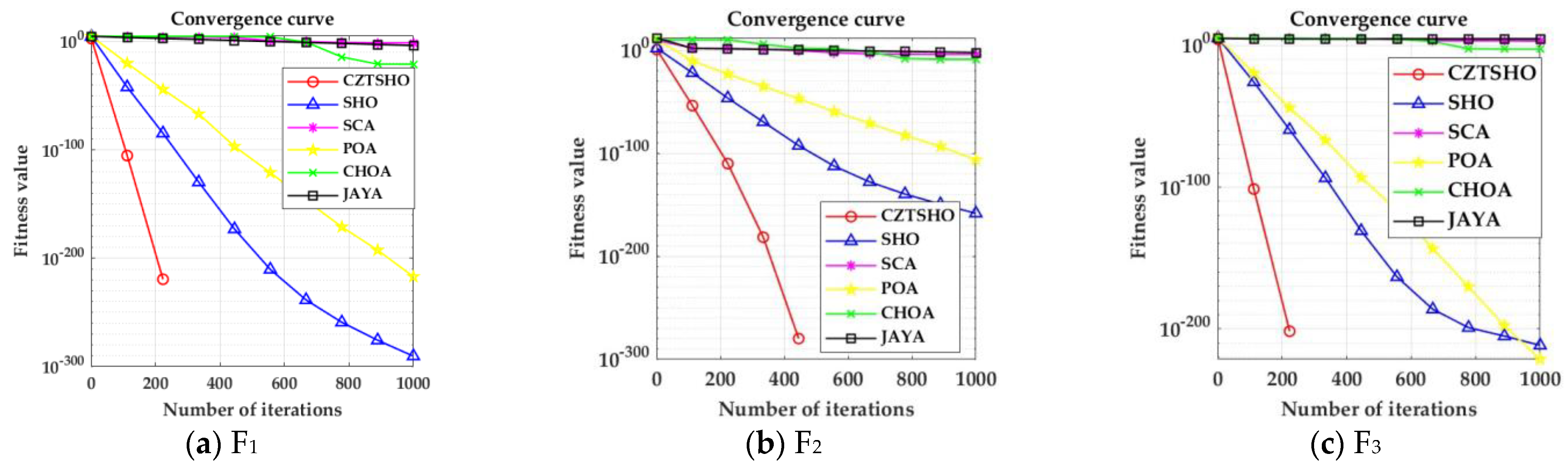
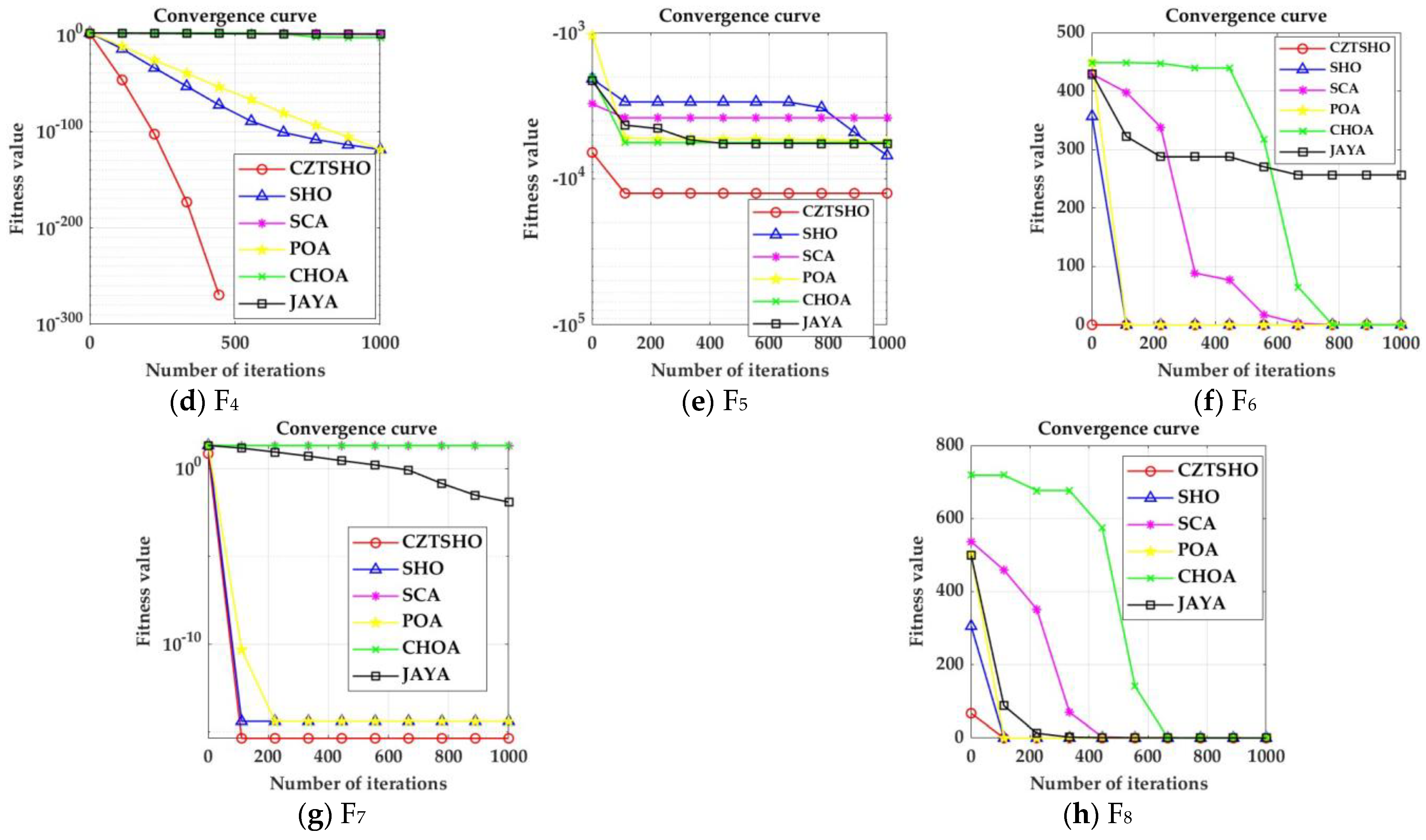
2.2.1. Benchmark Test Function

In order to test the optimization performance of the CZTSHO algorithm, 23 benchmark functions are used to test, and 8 basic functions are selected for simulation. In order to ensure the reliability of the algorithm, the benchmark functions include unimodal and multimodal functions, as shown in

Table 1. The 8 benchmark functions.

Function Expression	Hunting Zone
$F_1\left(x\right)=\sum _{i=1}^n{x}_i^2$	[−100, 100]
$F_2\left(x\right)=\sum _{i=1}^n\left|x_i\right|+\prod _{i=1}^n\left|x_i\right|$	[−10, 10]
$F_3\left(x\right)=\sum _{i=1}^n{\left(\sum _{j=1}^i{x}_j\right)}^2$	[−100, 100]
$F_4\left(x\right)={max}_i\left\{\left|x_i\right|,1\le i\le n\right\}$	[−100, 100]
$F_5\left(x\right)=\sum _{i=1}^n-x_i\sin \left(\sqrt{\left|x_i\right|}\right)$	[−500, 500]
$F_6\left(x\right)=\sum _{i=1}^n\left[x_i^2-10\cos (2\pi x_{i)}+10\right]$	[−5.12, 5.12]
$F_7\left(x\right)=-20\mathrm{e}\mathrm{x}\mathrm{p}\left(-0.2\sqrt{{\displaystyle \frac{1}{n}}\sum _{i=1}^n{x}_i^2}\right)-exp\left({\displaystyle \frac{1}{n}}\sum _{i=1}^n\cos \left(2\pi x_i\right)\right)+20+e$	[−32, 32]
$F_8\left(x\right)={\displaystyle \frac{1}{4000}}\sum _{i=1}^n{x}_i^2-\prod _{i=1}^n\cos \left({\displaystyle \frac{x_i}{\sqrt{i}}}\right)+1$	[−600, 600]

, where F₁~F₄ are unimodal benchmark functions, and F₅~F₈ are multimodal benchmark functions. The dimension of the solution space for the benchmark function is 30.

2.2.2. Performance Comparison and Test of CZTSHO Algorithm

In the performance test of the proposed CZTSHO algorithm, besides comparing with the standard SHO algorithm, POA [20], SCA, CHOA [21], and JAYA [22] are selected for optimization comparison on eight benchmark test functions to verify the superiority of the CZTSHO algorithm. In order to ensure the fairness of the simulation, the population number of each algorithm is set to 30, and the number of iterations is 1000. The search upper and lower bounds of the convergence curve are set according to the above eight benchmark test functions. The simulation environment is as follows: Windows S10 system, i7-8750H CPU, main frequency 2.2 GHz, 16 G running memory, and the simulation experiment is carried out on MATLAB R2023b. The convergence curves of six optimization algorithms on eight benchmark functions are shown in Figure 4.

Generally, the single-peak test function evaluates the development ability of the algorithm, and the multi-peak test function evaluates the search ability of the algorithm. In the single-peak test function F₁~F₄, CZTSHO and SHO are below other comparative optimization algorithms, indicating that the standard SHO algorithm has relatively fast convergence speed and optimization accuracy when dealing with the single-peak test function. The curve of the CZTSHO algorithm is below the standard SHO, indicating that the performance of the improved Seahorse Optimizer has been improved. In F₆, the CZTSHO, SHO, and POA algorithms converge at a similar speed, but CZTSHO maintains a high optimization accuracy. In F₈, the standard SHO algorithm is worse than the SCA, POA, CHOA, and JAYA algorithm, but, after improvement, the algorithm convergence and optimization performance are better than other algorithms; in F₉ and F₁₁, the improved algorithm convergence speed is higher than other algorithms, but after 100 iterations of the optimization, accuracy is similar; overall, it is proved that the improved CZTSHO algorithm has high optimization precision and good algorithm stability.

2.3. Water Quality Prediction Model of CZTSHO-HKELM

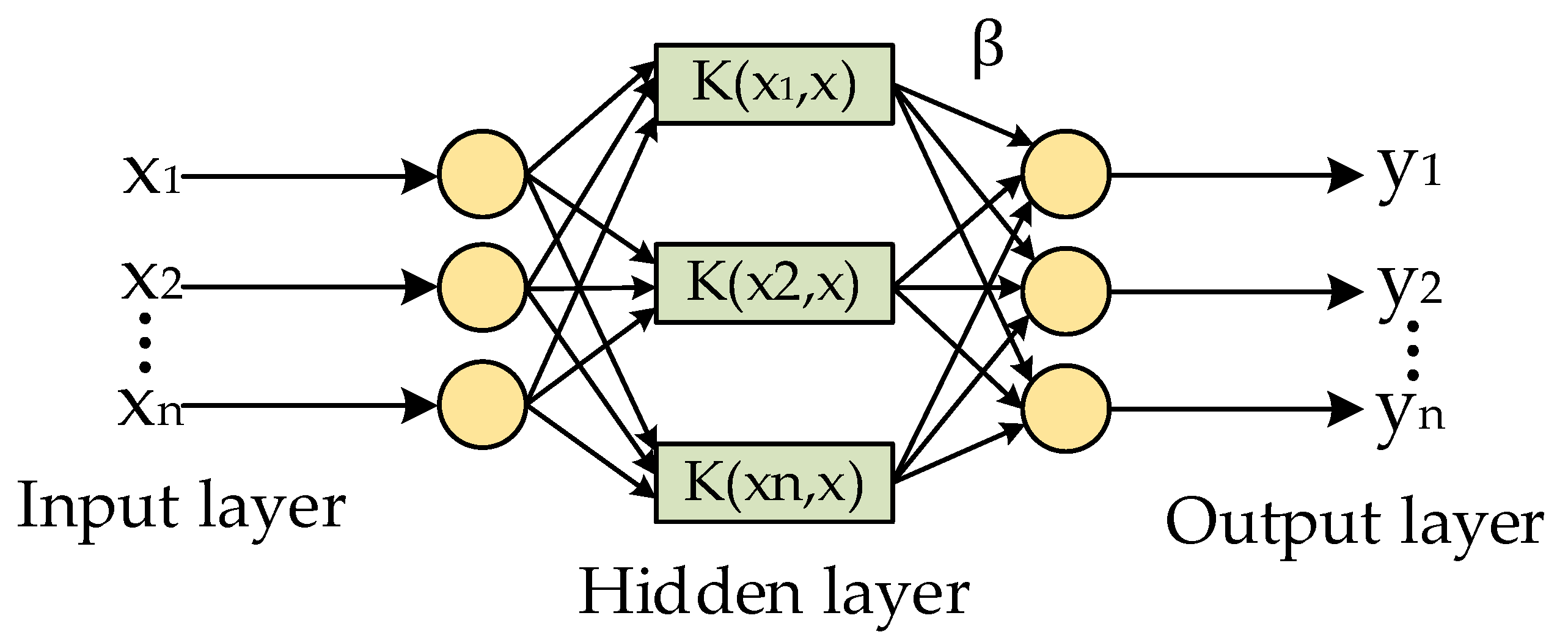
2.3.1. Hybrid Kernel Extreme Learning Machine

The extreme learning machine (ELM) is a fast learning method based on single hidden layer feedforward neural network. Its characteristics are that the weights and deviations of the input layer of the network are randomly selected, and the weights of the hidden layer and the output layer are determined with the least square method. Its prediction performance is not stable enough, its accuracy is limited, and it cannot be adjusted according to the characteristics of the dataset, and its controllable performance is poor. Therefore, this paper selects the kernel extreme learning machine (KELM) to replace the feature mapping of the ELM by introducing the kernel function, which improves the disadvantages of large randomness, has better convergence and generalization, and is better at solving the problem of regression prediction [23]. The model structure is shown in Figure 5.

For a given forecast sample, KELM’s forecast output is as follows:

$$f\left(x\right)=h\left(x\right)\beta =H\beta$$

(19)

where $f\left(x\right)$ is output and $x$ is sample data; $h\left(x\right)$ is the hidden layer input; $H$ is the feature mapping matrix; and $\beta$ is the vector that outputs the hidden layer data to the output layer:

$$\beta =H^T{\left({HH}^T+{\displaystyle \frac{I}{C}}\right)}^{-1}T$$

(20)

where $C$ is the regularization coefficient, $I$ and $T$ are the diagonal matrix and the sample output vector, respectively, and the matrix model of the extreme learning machine is shown as follows:

$$\left\{\begin{array}{c}{K}_{ELM}={HH}^T\\ K_{{ELM}_{i,j}}=h\left(x_i\right)h\left(x_i\right)=K\left(x_i,x_j\right)\end{array}\right.$$

(21)

Kernel matrix $K_{ELM}$ is used to replace $H{H}^T$ of the extreme learning machine to avoid setting the number of neurons in the hidden layer and randomly setting weights and biases.

Map the input data to the higher-dimensional hidden layer feature space, where $K(x_i,x_j)$ is the kernel function matrix, $x_1, x_2,\cdots x_n$ are the input vectors of the training set, and the output model can be obtained as follows:

$$f\left(x\right)={\left[\begin{array}{c}K\left(x,x_1\right)\\ ⋮\\ K\left(x,x_N\right)\end{array}\right]}^T{\left(K_{ELM}+{\displaystyle \frac{I}{C}}\right)}^{-1}T$$

(22)

It can be seen that different choice of kernel function directly determines the performance of prediction, and it is difficult to apply a single kernel function to a multi-feature input such as water quality data. There are many types of kernel functions, among which the radial basis function (RBF) is a local kernel function with strong learning ability. The polynomial kernel function (Poly) is a global kernel function with strong generalization ability. Therefore, two different types of kernel functions were combined with variable weights to form a mixed kernel function, and a prediction model based on a hybrid kernel extreme learning machine (HKELM) was constructed [24], so as to better learn the nonlinear relationship between dissolved oxygen and other characteristic factors in water quality data. The calculation formula of the two kernel functions is as follows:

$$K_{RBF}\left(x_i,x_j\right)=\mathrm{e}\mathrm{x}\mathrm{p}\left({\displaystyle \frac{-{{\Vert x}_i-x_j\Vert }^2}{2{\sigma }^2}}\right)$$

(23)

$$K_{Poly}\left(x_i,x_j\right)={\left(x,x_i+c_1\right)}^d$$

(24)

$$K_{HK}\left(x_i,x_j\right)=\mu K_{RBF}\left(x_i,x_j\right)+\left(1-\mu \right)K_{Poly}\left(x_i,x_j\right)$$

(25)

where $\sigma$ is the nuclear parameter of the RBF nucleus; $c_1,d$ is the nuclear parameter of the Poly nucleus, $\mu$ is the weight coefficient between the two nuclei, and $\mu \in \left(\mathrm{0,1}\right)$.

It can be seen from the formula that there are many parameters in the HKELM model, and different parameters have a great impact on the accuracy of the model. CZTSHO is used to optimize the parameters of the HKELM model to improve the prediction performance.

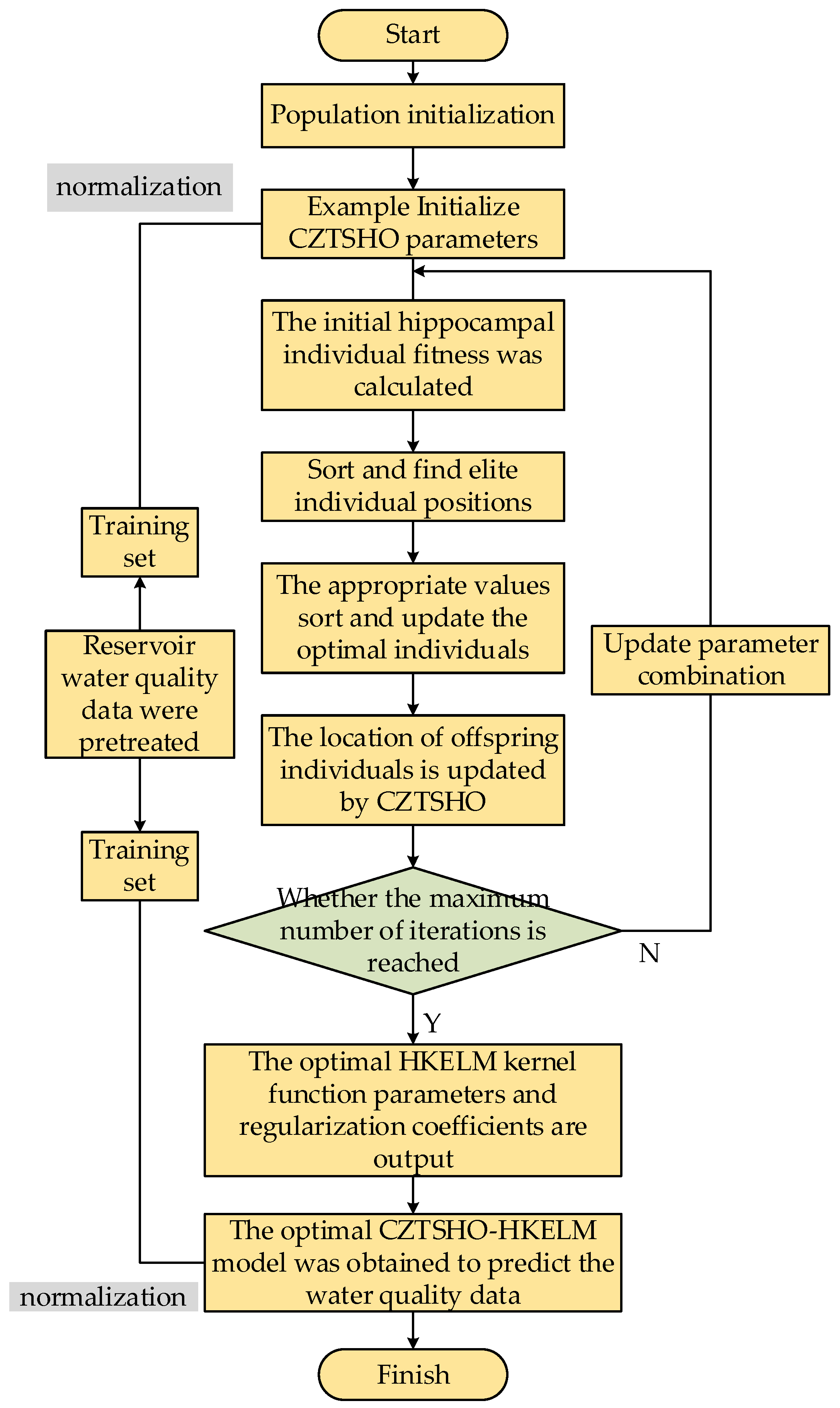
2.3.2. Optimization of Water Quality Prediction Steps of HKELM via the Improved Seahorse Optimizer

The data of reservoir water quality is complex and easily influenced by external factors, and the traditional water quality prediction method has limitations and low prediction accuracy. This paper proposes a CZTSHO–HKELM prediction model and optimizes the parameters of HKELM through an improved Seahorse Optimizer. The steps are as follows:

(1)

Obtain the monitored water quality data, conduct data analysis (introduced in the next chapter), divide the proportion of training set and test set, input the feature dimension, and normalize the data;

(2)

Initialize CZTSHO parameters: set the population size to 30, the maximum number of iterations is 500, and set the optimized upper and lower bounds and dimensions;

(3)

Set the parameters of the HKELM: take the regularization coefficient C, the kernel parameter $\sigma$ of the RBF kernel function, the parameters $c_1$ and $d$ of the Poly kernel function, and the mixed weight coefficient $\mu$;

(4)

Calculate the fitness of hippocampus individuals, sort them to find the position of elite individuals, and judge the search mode. Sine and cosine strategies are used to replace predation behavior, and lens imaging reverse learning is used to generate offspring, and then the position of predator offspring is updated according to the CZTSHO update formula;

(5)

Determine whether the maximum number of iterations is reached, if not, update the parameter combination and return to step (4); if the maximum number of iterations is reached, the optimal parameter model is retained, and the optimization ends.

The specific process is shown in Figure 6.

3. Experiment and Result Analysis

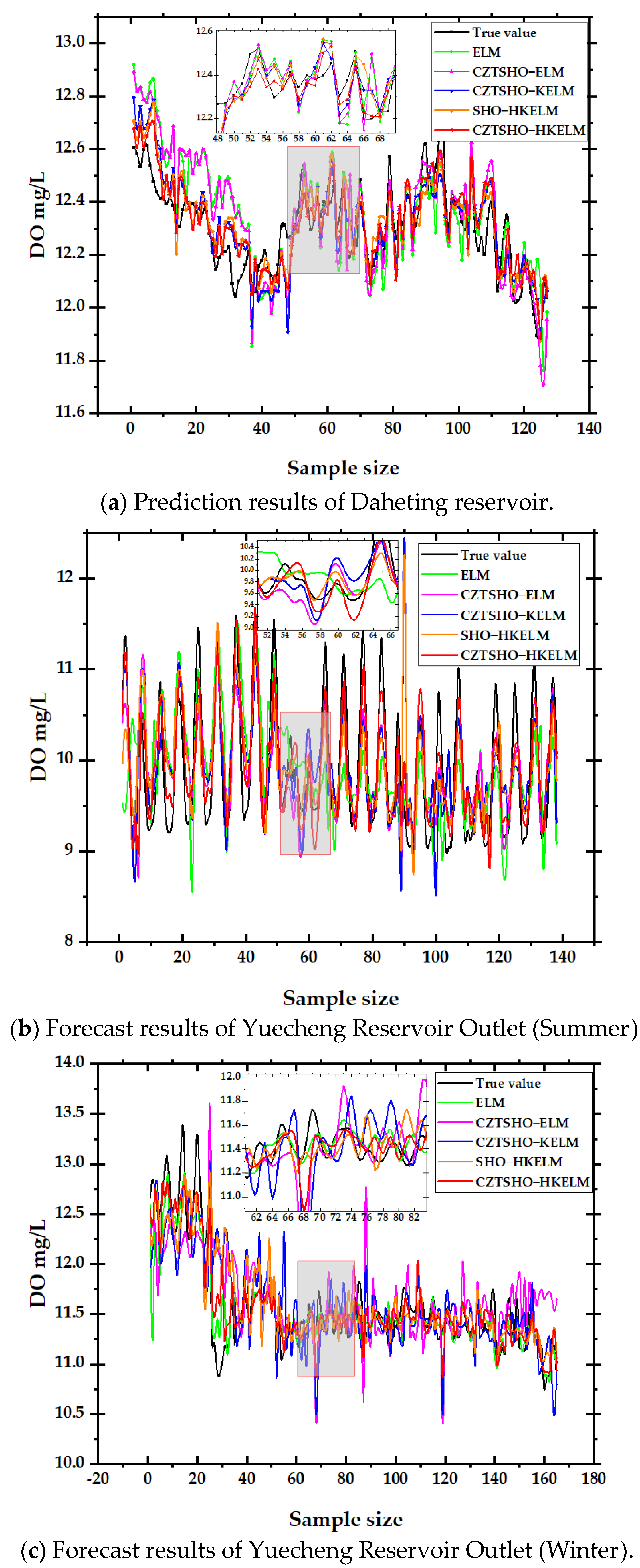
In order to verify the effectiveness of the proposed method, actual water quality data are used in the example. Since the water quality data of the reservoir is affected by the flow state, season, and depth of the lake and reservoir, three kinds of water quality data from different seasons and different locations are selected for experimental analysis. The data are from water quality monitoring information released by the China General Environmental Monitoring Station (https://www.cnemc.cn/) (accessed on 1 December 2023). A total of 638 datasets were sampled and published every 4 h from Daheting Reservoir from 1 January 2023 to 30 April 2023, a total of 689 datasets were sampled and published every 4 h from the exit of Yuecheng Reservoir from 1 July 2022 to 31 October 2022, and a total of 826 were sampled and published every 4 h from Yuecheng Reservoir from 1 November 2022 to 31 March 2023, including eight water quality indexes: water temperature (T), pH, potassium permanganate (KMnO4), ammonia nitrogen content (NH₃-N), total phosphorus content (TP), total nitrogen content (TN), electrical conductivity (EC), and turbidity (SS).

Figure 7 shows the scatter diagram of water quality data (part) from Daheting Reservoir for the period from 1 January 2023 to 30 April 2023. It can be seen that the concentration of dissolved oxygen exhibits significant fluctuations over time, while some water quality data, such as TP and SS, contain abnormal values. Overall, the performance of EC remains relatively stable. Descriptive statistics for all data (water quality parameters) are shown in

Table 2. Descriptive statistics for water quality parameters.

Variable	Mean	SD	Min	Max	Median	Skewness	Kurtosis
DO	12.62	0.38	9.17	13.95	12.56	−0.83	12.14
EC	603.87	56.92	0.47	636.06	616.77	−9.20	94.70
NH3-N	0.04	0.03	0.03	0.80	0.04	19.00	435.05
SS	1.35	0.81	0.23	4.57	1.20	1.95	3.50
T	5.58	3.33	1.48	22.56	4.35	1.08	0.62
TN	4.87	0.33	0.50	7.19	4.93	−3.14	49.82
TP	0.02	0.00	0.01	0.03	0.02	0.10	−0.05
pH	8.16	0.09	7.05	8.37	8.16	−2.56	35.31

.

During data collection, it is inevitable to encounter abnormal values or loss, resulting in prediction errors. Firstly, the collected data are preprocessed, and the abnormal data are mainly measured by $3\sigma$. If the input data are not within the normal range, they are considered abnormal and will be replaced by the mean value. The interpolation method was used to fill in the missing data. Since the seven parameters T, PH, NH3-N, TP, TN, EC, and SS had a great impact on DO, these seven parameters were selected as input samples. In addition, there are many factors affecting DO concentration and different data have different ranges. This paper will adopt normalization processing, map the data to $[0,1]$, and finally reverse normalize the output data to obtain the predicted value of the corresponding model. Data normalization aims to unify the numerical ranges of different features so that neural network models can learn and converge more efficiently. Scaling the raw data to a specified range can be achieved using the following formula:

$$x^{\prime }={\displaystyle \frac{x-\mathit{min}\left(x\right)}{\mathit{max}\left(x\right)-\mathit{min}\left(x\right)}}$$

(26)

$x$ is the raw data, $x^{\prime }$ is normalized data, $min\left(x\right)$ is the minimum value of the data, and $max\left(x\right)$ is the maximum value of the data. The purpose of data normalization is to eliminate differences in dimensionality and numerical range between different features, so that the neural network model can learn data features more stably and efficiently. The normalized data help to accelerate the convergence speed of the model, reduce the training time, and improve the prediction accuracy and generalization ability of the model. Additionally, 80% of the data are used as the training set and 20% as the test set.

In order to better display the prediction accuracy of the proposed method, a comparative simulation was conducted with ELM, CZTSHO–ELM, CZTSHO–KELM, and SHO–HKELM, respectively, to verify the prediction accuracy of the CZTSHO–HKELM prediction model proposed in this paper, in which ELM is a single extreme learning machine model. CZTSHO–ELM optimizes the extreme learning machine model to improve the Seahorse Optimizer. CZTSHO–KELM optimized the kernel extreme learning machine model with the RBF kernel function to improve the Seahorse Optimizer. SHO–HKELM optimized the hybrid core extreme learning machine for the original Seahorse Optimizer. In order to reduce the chance of neural network optimization and improve the errors caused by some random numbers in the seahorse algorithm, three repeated and independent simulations were used to take average values. The prediction results are shown in Figure 8.

To visualize the prediction effect more intuitively, the outlet of Yuecheng Reservoir (winter) is selected as an example. A scatter plot is created with the true values on the horizontal axis and the predicted values on the vertical axis. Additionally, a reference straight line $y=x$ is drawn, representing where the predicted values are exactly equal to the true values, as shown in Figure 9.

For different water quality data, the water quality conditions vary. The network needs to set hyperparameters specific to the current data. The intelligent optimization algorithm can adaptively adjust these network hyperparameters. For different models, the CZTSHO algorithm is used to optimize the corresponding important hyperparameters. Taking Daheting Reservoir as an example, the optimization parameters for different models are shown in

Table 3. Hyperparameters from different model optimizations.

Network Model	Hyperparameter
ELM	$Number of hidden layer nodes=50$
CZTSHO–ELM	$Max\text{\_}iterations=500,pop=30$
CZTSHO–KELM	$C=50,\sigma =1$
SHO–HKELM	$C=1.094, \sigma =0.05,c_1=5.30,d=3.91,\mu =0.25$
CZTSHO–HKELM	$C=13.67,\sigma =0.03,c_1=47.04,d=1.84,\mu =0.37$

.

As can be seen from Figure 8 and Figure 9, the predicted value of ELM has the largest error with respect to the true value in three different cases. The prediction effect of CZTSHO–ELM is poor when the data fluctuate greatly. The predicted value of the CZTSHO–KELM and SHO–HKELM models is close to the actual curve, but the prediction accuracy is relatively low, and the error is large. The CZTSHO–HKELM model has the highest fit and prediction accuracy with the actual value, and the concentration of dissolved oxygen will decrease with the increase of temperature, and the concentration of dissolved oxygen in different reservoirs is also affected by external factors. In summer, the difference in dissolved oxygen content with respect to water quality between morning and evening is large, resulting in large fluctuation in the image, and the prediction effect will be reduced to a certain extent.

In order to verify the performance of the proposed model, the loss function can be used as the evaluation criteria, including the root mean square error (RMSE), mean absolute error (MAE), and determination coefficient R².

The evaluation metrics for each prediction model, calculated using the formula on the test set, are shown in

Table 4. The prediction error of each model for the test set.

Locations	Model	RMSE	MAE	R2
Daheting Reservoir	ELM	0.135	0.101	0.841
	CZTSHO–ELM	0.120	0.091	0.888
	CZTSHO–KELM	0.096	0.067	0.918
	SHO–HKELM	0.089	0.064	0.919
	CZTSHO–HKELM	0.077	0.057	0.954
Yuecheng Reservoir Outlet (Summer)	ELM	0.946	0.718	0.543
	CZTSHO–ELM	0.917	0.644	0.572
	CZTSHO–KELM	0.775	0.591	0.674
	SHO–HKELM	0.748	0.559	0.731
	CZTSHO–HKELM	0.561	0.406	0.849
Yuecheng Reservoir Outlet (Winter)	ELM	0.511	0.258	0.661
	CZTSHO–ELM	0.441	0.348	0.726
	CZTSHO–KELM	0.391	0.261	0.763
	SHO–HKELM	0.371	0.257	0.815
	CZTSHO–HKELM	0.261	0.182	0.898

Note: The units for both RMSE and MAE are Mg/L.

.

The Taylor chart provides a framework for visually comparing the performance of different models or observational datasets and shows the correlation between the data. Since the optimization algorithm involves some randomly generated numbers, we conducted several experiments and averaged the results to create the Taylor chart, as shown in Figure 10. In the chart, REF represents the reference model.

In addition, we generated a violin diagram based on the prediction results, which more intuitively illustrates the effects of different prediction models, as shown in Figure 11.

Combining different kinds of graphs and prediction results and tables, we can see the following:

(a)

The proposed hybrid model can achieve high prediction accuracy and closely aligns with the original sequence. It can also make accurate predictions for the two seasons with significant differences in data levels, indicating that the model has strong universality and generalization. Although all models can predict the change trend of the true value, there are still fitting errors at sample points with a large fluctuation range, and the prediction accuracy of a single extreme learning machine is poor. The coefficient of determination (R²) at the outlet of Yuecheng Reservoir in summer is only 0.543;

(b)

Taking the Daheting Reservoir as an example, the improved Seahorse Optimizer optimized the extreme learning machine and kernel extreme learning machine, respectively, and the unimproved Seahorse Optimizer optimized the hybrid kernel extreme learning machine. Compared with the ELM, the RMSE was reduced by 11.1%, 20.0%, and 25.8%, MAE was reduced by 9.9%, 26.3%, and 29.6%, and R² was improved by 5.5%, 3.3%, and 3.4%, while the ELM using the improved Seahorse Optimizer to optimize the hybrid kernel function had a 35.8% reduction in RMSE, a 37.3% reduction in MAE, and a 7.4% increase in R² compared with other models. It has the highest prediction accuracy and the largest determination coefficient, and its performance is better than other models. It is more suitable for predicting data with strong volatility such as water quality;

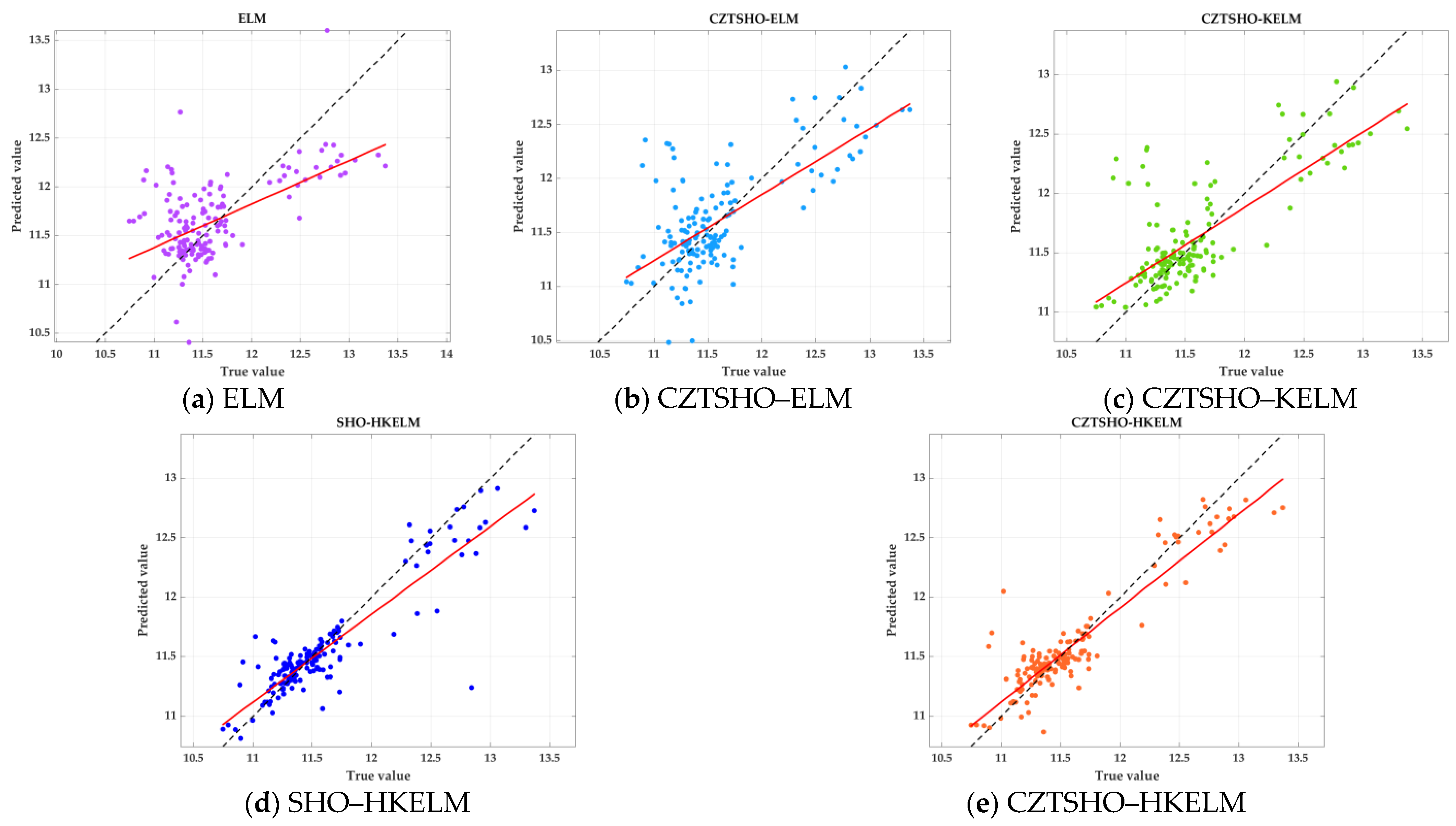
(c)

From the scatter plot, we can see that the smaller the angle between the regression line of each model and $y=x$, the better the prediction effect. Clearly, the ELM has the largest angle with $y=x$ and the worst prediction effect. As model complexity and algorithm improvements increase, the angle gradually becomes smaller, and prediction accuracy improves. CZTSHO–HKELM is very close to this straight line, indicating that it is the optimal model. When the dissolved oxygen value is around 11–12, the predicted values of each model are closer to the actual values. However, after exceeding 12, the effectiveness of each model decreases slightly;

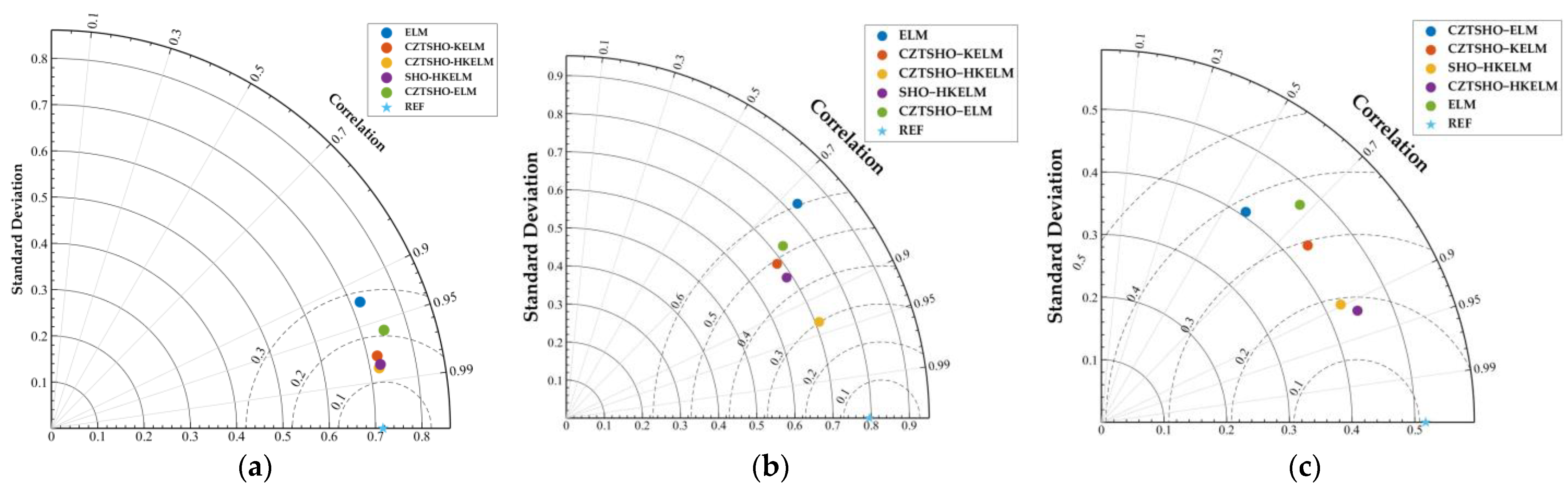
(d)

From the Taylor diagram and violin plot, it can be seen that CZTSHO–HKELM has the best performance among the compared models, with correlations ranging between 0.9 and 0.95. In contrast, SHO-HKELM and CZTSHO-KELM exhibit similar prediction effects at Daheiting Reservoir, with correlations around 0.8. However, the prediction effects differ at the outlet of the Yuecheng Reservoir in winter and summer. Both models are susceptible to data fluctuations, with the ELM showing a correlation as low as 0.7;

(e)

The evaluation standard of the summer and winter models at the outlet of Yuecheng Reservoir is the same as that of Daheiting Reservoir, and CZTSHO-HKELM has the best prediction effect, which shows that the prediction model of hybrid kernel extreme learning machine optimized with the improved Seahorse Optimizer can accurately predict the dissolved oxygen concentration in water quality in different reservoirs or rivers and in different seasons, effectively reflecting the water quality parameters. The model exhibits lower error in winter compared to summer and is less affected by abrupt weather changes and other factors. Additionally, the model can be used to predict other water quality parameters, such as ammonia nitrogen and conductivity, and can also be applied to other fields, such as wind speed and runoff prediction.

4. Conclusions

In view of the fluctuation and randomness of water quality data, a prediction model of dissolved oxygen content in water quality optimized with the SHO in the HKELM was proposed, and the following conclusions were drawn:

(1)

The Seahorse Optimizer, improved by circle chaos mapping, the sine–cosine strategy, and lens imaging reverse learning strategy, enhances the ergodic properties of the population, increases the randomness of the search, and improves the global search capability. It can also prevent hippocampal individuals from falling into local optima and demonstrates that the optimal solution can be reached in about 200 iterations for the selected eight benchmark functions, whereas other algorithms may require up to 600 iterations to achieve the optimal value;

(2)

The experimental results show that the water quality prediction model based on CZTSHO–HKELM outperforms CZTSHO–KELM, CZTSHO–KELM, CZTSHO–ELM, and the ELM in terms of prediction accuracy (such as the RMSE and MAE) and exhibits the strongest correlation, and the HKELM can extract deep information in water quality time series, overcoming the limitation of the ELM model with which it is difficult to capture high correlation features due to the single-hidden-layer structure. Compared with other models, the RMSE and MAE are reduced under three different water quality conditions, and the prediction accuracy is improved, and the model has the ability to accurately predict water quality parameters under different water quality and external conditions;

(3)

For different reservoirs, influenced by factors such as water flow state and reservoir depth, the model maintains good accuracy. The prediction results are scientifically sound and effectively reflect water quality parameters, which is crucial for water environment protection. However, within the same reservoir, seasonal temperature variations impact prediction accuracy. In summer, the large temperature differences between day and night lead to reduced accuracy and increased error, while in winter, the smaller temperature differences have minimal impact on the prediction effectiveness.

In future studies, we can explore the impact of variational mode decomposition on various pollution factor prediction models beyond DO and delve deeper into processing the original data. In summary, water quality prediction is a crucial aspect of environmental management and water resource protection with broad research prospects. With ongoing advancements in technology, progress and innovation are expected, and the application of deep learning, neural networks, and intelligent technologies will further enhance the accuracy and efficiency of water quality prediction. Additionally, growing policy support and market demand provide impetus for the development of the water quality monitoring industry, which is of great significance for the protection of the global water environment.

References

1. Valadkhan, D.; Moghaddasi, R.; Mohammadinejad, A. Groundwater quality prediction based on LSTM RNN: An Iranian experience. Int. J. Environ. Sci. Technol. 2022, 19, 11397–11408. [Google Scholar] [CrossRef] [PubMed]
2. van Vliet, M.T.H.; Thorslund, J.; Strokal, M.; Hofstra, N.; Flörke, M.; Ehalt Macedo, H.; Nkwasa, A.; Tang, T.; Kaushal, S.S.; Kumar, R.; et al. Global river water quality under climate change and hydroclimatic extremes. Nat. Rev. Earth Environ. 2023, 4, 687–702. [Google Scholar] [CrossRef]
3. Li, R.; Zhu, G.; Lu, S.; Sang, L.; Meng, G.; Chen, L.; Jiao, Y.; Wang, Q. Effects of urbanization on the water cycle in the Shiyang River basin: Based on a stable isotope method. Hydrol. Earth Syst. Sci. 2023, 27, 4437–4452. [Google Scholar] [CrossRef]
4. M, G.J. Secure water quality prediction system using machine learning and blockchain technologies. J. Environ. Manag. 2024, 350, 119357. [Google Scholar] [CrossRef] [PubMed]
5. Li, J.; Lei, Y.; Yang, S. Mid-long term load forecasting model based on support vector machine optimized by improved sparrow search algorithm. Energy Rep. 2022, 8, 491–497. [Google Scholar] [CrossRef]
6. Gai, R.; Zhang, H. Prediction model of agricultural water quality based on optimized logistic regression algorithm. EURASIP J. Adv. Signal Process. 2023, 2023, 21. [Google Scholar] [CrossRef]
7. Banda, T.D.; Kumarasamy, M. Artificial Neural Network (ANN)-Based Water Quality Index (WQI) for Assessing Spatiotemporal Trends in Surface Water Quality—A Case Study of South African River Basins. Water 2024, 16, 1485. [Google Scholar] [CrossRef]
8. Yan, J.; Liu, J.; Yu, Y.; Xu, H. Water Quality Prediction in the Luan River Based on 1-DRCNN and BiGRU Hybrid Neural Network Model. Water 2021, 13, 1273. [Google Scholar] [CrossRef]
9. Huang, G.-B.; Wang, D.H.; Lan, Y. Extreme learning machines: A survey. Int. J. Mach. Learn. Cybern. 2011, 2, 107–122. [Google Scholar] [CrossRef]
10. Anmala, J.; Turuganti, V. Comparison of the Performance of Decision Tree (DT) Algorithms and ELM model in the Prediction of Water Quality of the Upper Green River watershed. Water Environ. Res. A Res. Publ. Water Environ. Fed. 2021, 93, 2360–2373. [Google Scholar] [CrossRef]
11. Javad, A.; Ewees, A.A.; Sepideh, A.; Shamsuddin, S.; Mundher, Y.Z. A new insight for real-time wastewater quality prediction using hybridized kernel-based extreme learning machines with advanced optimization algorithms. Environ. Sci. Pollut. Res. Int. 2021, 29, 20496–20516. [Google Scholar]
12. Liu, T.; Liu, W.; Liu, Z.; Zhang, H.; Liu, W. Ensemble water quality forecasting based on decomposition, sub-model selection, and adaptive interval. Environ. Res. 2023, 237, 116938. [Google Scholar] [CrossRef]
13. Pang, J.; Luo, W.; Yao, Z.; Chen, J.; Dong, C.; Lin, K. Water Quality Prediction in Urban Waterways Based on Wavelet Packet Denoising and LSTM. Water Resour. Manag. 2024, 38, 2399–2420. [Google Scholar] [CrossRef]
14. Zhao, S.; Zhang, T.; Ma, S.; Wang, M. Sea-horse optimizer: A novel nature-inspired meta-heuristic for global optimization problems. Appl. Intell. 2022, 53, 11833–11860. [Google Scholar] [CrossRef]
15. Arora, S.; Anand, P. Chaotic grasshopper optimization algorithm for global optimization. Neural Comput. Appl. 2018, 31, 4385–4405. [Google Scholar] [CrossRef]
16. Herbadji, D.; Derouiche, N.; Belmeguenai, A.; Herbadji, A.; Boumerdassi, S. A Tweakable Image Encryption Algorithm Using an Improved Logistic Chaotic Map. Trait. Signal 2019, 36, 407–417. [Google Scholar] [CrossRef]
17. Ge, Z.; Feng, S.; Ma, C.; Dai, X.; Wang, Y.; Ye, Z. Urban river ammonia nitrogen prediction model based on improved whale optimization support vector regression mixed synchronous compression wavelet transform. Chemom. Intell. Lab. Syst. 2023, 240, 104930. [Google Scholar] [CrossRef]
18. Mirjalili, S. SCA: A Sine Cosine Algorithm for solving optimization problems. Knowl.-Based Syst. 2016, 96, 120–133. [Google Scholar] [CrossRef]
19. Li, Y.; Sun, K.; Yao, Q.; Wang, L. A dual-optimization wind speed forecasting model based on deep learning and improved dung beetle optimization algorithm. Energy 2024, 286, 129604. [Google Scholar] [CrossRef]
20. Trojovský, P.; Dehghani, M. Pelican Optimization Algorithm: A Novel Nature-Inspired Algorithm for Engineering Applications. Sensors 2022, 22, 855. [Google Scholar] [CrossRef]
21. Khishe, M.; Mosavi, M.R. Chimp Optimization Algorithm. Expert. Syst. Appl. 2020, 149, 113338. [Google Scholar] [CrossRef]
22. Rao, R.V. Jaya: A simple and new optimization algorithm for solving constrained and unconstrained optimization problems. Int. J. Ind. Eng. Comput. 2016, 7, 19–34. [Google Scholar]
23. Zhang, Q.; Tsang, E.C.C.; Hu, M.; He, Q.; Chen, D. Fuzzt Set-Based Kernel Extreme Learning Machine Autoencoder for Multi-Label Classification. In Proceedings of the 2021 International Conference on Machine Learning and Cybernetics (ICMLC), Adelaide, Australia, 4–5 December 2021; pp. 1–6. [Google Scholar]
24. Li, J.; Hai, C.; Feng, Z.; Li, G. A Transformer Fault Diagnosis Method Based on Parameters Optimization of Hybrid Kernel Extreme Learning Machine. IEEE Access 2021, 9, 126891–126902. [Google Scholar] [CrossRef]
Figure 1. Circle chaotic map distribution and histogram.
Water 16 02232 g001
Figure 2. Schematic diagram of lens imaging reverse learning strategy.
Water 16 02232 g002
Figure 3. Flow chart of improved Seahorse Optimizer.
Water 16 02232 g003
Figure 4. Convergence curves of 6 algorithms on 8 representative test functions.
Water 16 02232 g004aWater 16 02232 g004b
Figure 5. KELM model structure topology diagram.
Water 16 02232 g005
Figure 6. Water quality forecasting process.
Water 16 02232 g006
Figure 7. Scatter plot of reservoir water quality data (part).
Water 16 02232 g007
Figure 8. Comparison of model prediction results.
Water 16 02232 g008
Figure 9. Scatter plot of prediction results from different models.
Water 16 02232 g009
Figure 10. Taylor diagram of prediction results from different models. (a) Daheting Reservoir. (b) Yuecheng Reservoir Outlet (Summer). (c) Yuecheng Reservoir Outlet (Winter).
Water 16 02232 g010
Figure 11. Violin diagram of the results from different model predictions. (a) Daheting Reservoir. (b) Yuecheng Reservoir Outlet (Summer). (c) Yuecheng Reservoir Outlet (Winter).
Water 16 02232 g011